Statistical Analysis of Reliability Data in Randomly Censored Life Testing

Journal of the Operations Research SOciety of Japan

Vol. 23, No. 3, September 1980

STATISTICAL ANALYSIS OF RELIABILITY DATA IN

RAMDOMLY

CENSORED

LIFE TESTING

Tetsuc Miyamura Ibaraki University (Received November 9,1978)

Abstract For independent nonnegative continuous random variables Xl, . . . , Xb Z = min (Xl, ... , Xk) and fj;(i=1, ... , k), where fji = 1 if Z = Xi and fji = 0 otherwise, are statistically independent random variables if and only if the distribution of Xi is written as Fi(X) = 1 - exp(-piQ(X)) (i=1, ... , k). From this characterization theorem for the random variable Xi, an unbiased estimate for failure rate of distribution function is presented using reliability data in random life testing. A saving of time in a life testing experiment by allowing random censoring is also discussed.

1. Introduction

In reliability analysis, it is practically important to know the failure characteristics of the components which compose the system, either as a "se-ries system" (where the system fails if any component fails), or a "parallel system" (where the system fails only F all components fail). Usually they may be estimated properly from the component test data and, therefore, a great number of papers have been devoted to ·:he matter.

In some cases, however, the serieB system data are available for estimat-ing the probability of failure for each of the components. Here, the system data may be consist of two kinds of sel:S: one is the time-to-failure of the system and the other the cause of the Bystem failure, which implies that the system failure is occured by the failure of the one of k independent, but dif-ferent components.

To illustrate the situation, we consider an integrated circuit (IC) in the area of a semi-conductor. When the IC is connected with an external ter-minal, the surface of the alminum electrode is contacted with the external gold line by the method of thermal compression. In this life test, the gold line is pulled for the purpose of measuring the strength of contactness

(de-} 91

noted by

Xl)'

and then the value of

Xl

is observed if X1~ the strength of the gold line (denoted by

X

2

):

otherwise, just the information that

X

l

>X

2

is

pro-vided. After all we observe

Z=min(X

1

.X

2) and the cause of the breakdown, which means that our observation is based upon either Xl or X₂.

In this article, estimation of the failure characteristics of the compo-nent under random censorship will be considered. Random censorship means that the observable value is restricted to (Z

=

min(Xl' ..•• X7<.)'

Z

=

Xi)

= (age of fail-ure, cause of failure) where

X

1

•...• X7<.

are independent nonnegative continuous

random variables. The model arises from many practical situations such as medical follow-up studies, competing risks except life testing stated as above.

Notations and assumptions are stated in Section 2. In section 3 a chara-cterization of distribution function is constructed: the charachara-cterization theo-rem is related to the theotheo-rem due to Berman[2]. Section 4 contains applica-tions of the characterization theorem. An unbiased estimate for failure rate of distribution function is presented and some comparisons of efficiency of this estimate with the minimum variance unbiased estimate under Type

n

censored data are made. These comparisons show that randomly censored life testing gives much more information per unit time than Type

n

censoring when underlying distribution is Weibull with the shape parameter m~ 1.

to related works.

2. Notations and Assumptions

Section 4 is devoted

It is assumed that a system is composed of 7<. independent, but non-identi-cal components in a series. If X

.(i=

1 •...• 7<.) is a nonnegative continuous

"/..

random variable indicating the life of the ith component, the life of the se-ries system is represented by the following way: that is,

Z

=

min(X

1 • . • . •

X7<.).

For

i=

1 •••.• 7<., denote F.(x) = P(X.?x) "/.. "/.. Conveniently we put R.(x) = 1 - F.(x) "/.. "/..

(i=1 •...• 7<.)

and define a new measure Q.(x) by the relation "/..

R .( x) = exp { -Q. (x) }

"/.. "/..

(i=

1.···

.7<.)

It is obvious that there exist one-to-one correspondence between Q.(x) and "/..

R.(x).

where

Statistical Analysis uf Randomly Censored Data

F(x) = NZ~x) k 1- exp{- E li.(x)} i=l "Z-R(x) = 1-F(x) = exp{-Q(x)} k Q(x) = E Q.(x). i=l "Z-1-exp{-Q(x)} 193

Suppose that observations are to be taken from the distribution of Z with the restriction that the value of X. can be observed if and only if X.~Z;

"Z-

"Z-otherwise just information that Xi >;~ is provided. From a sample of observa-tions with this sort of random censo::ing, it is required that an inference be made about the parameters of each of the random variables

X

1

.···.X

k

.

The details of observations are represented in the following way. We as-sume that the series systems have bel!n subjected to life test until the time of the 1'th failure with Type

:n:

censoring at l' out of n. For the system, we

ob-serve

Zl<Z2<"'<Z1" (1' > 2)

where

z.

is the jth smallest failure time of the l' failures of the system. To

J

apply a binomial sampling plan to this situation, define the random variable

1

o

•

i f Xi~ Z

i f

x.

> Z

"Z-for i = l ...

·.k.

and the joint distribution function of O. and Z

"Z-G.(x)

=

No.=l. Z~x) "Z-

"Z-Clearly, the random variable

O.

has a binomial distribution with the parameter

"Z-p. = P(o.=l) = P(X.2:Z) " z - " z - "Z- =

J'"

c' IT {l-F,{t)}dF.(t)

#i

J

"Z-For a given, positive integer 1', it i.s assumed that the failures of the ith component are observed 1'. times: that: is,

"Z-where 0 .. "Z-J l'

Eo ..

j=l "Z-J 1 {

o •

•

l ' i f Xij~ Zj i f

x . .

> Z. "Z-J J k E 1', i=l 2,

Remark 1.

In the life table, let Xl denote the true survival time for an individual and X

That is, the Xl is censored on the right by the X

2 since one observes only

and

6

where 6 indicates whether Xl is censored (6= 0) or not (6= 1).

Remark 2.

Considering a competing risks study in which it is presumed that there are

k

risks of death competing for the life of an individual. Upon death, the age and cause of death are recorded (Z= min(X

1,··· ,Xk), Z= Xi)' Based on these data one wishes to examine and predict the mortality pattern under the hypothetical conditions when certain risks of death are e1minated.

3. Fundamental Theorem

We will be concerned with the case where 6. (i = 1, •.. , k) and Z are

inde-1..

pendent random variables. Although the set

{6.}

and

Z

are not independent in

1..

general, Theorem below shows that

{6.}

and

Z

are independently distributed if

1..

and only i f F.(x) is written as F.(x) = 1-exp{-p.Q(x)} for i= 1,···,k

1.. 1.. 1..

Lemma due to Berman[2] is needed for the proof of Theorem.

Lemma.

(Berman[2]) The set of functions {F.(x)} is given by

1..

F.(x)

=

1-exp{-f x

(l-

~

G.(t))-l dG .(t)}

1.. 0 j=l J 1..

using the set {G.(x)}.

1..

(3.1)

If

{6.}

and

Z

are independent, then G.(x) is written as

1.. 1.. G.(X) = P(6.=l)·P(Z~x) 1.. 1.. = p.{l-exp{-Q(x)}} 1.. for i= 1,· .. ,k . be constructed.

Applying Equation (3.1) and Lemma the following theorem can

Theorem.

A necessary and sufficient condition for {6.} and Z to be

inde-1..

pendent is that F.(x) is given by F.(x)=l-exp{-p.Q(x)} for i = l , ... , k .

1.. 1.. 1..

Proof:

To see that the condition is necessary, we assume {6.} and Z to

1..

be independent, that is, G.(x)=p.F(x) for i = l , · · · , k .

1.. 1.. lemma, F .(x) 1..

r

x k 1 1-exp{- (1-

L

G.(t))- dG.(t)} 10 j=l J 1.. PidF(t)

- - - }

k .1- L p .F(t) j=l J

Statistical Analysis of Randomly Censored Data 195

f

x dF(t) l-exp{-p. _ _ } '/; 0 R(t) By applying Q(x)

=

J:

dF(t)/R(t) , we have F.(x)

=

l-exp{-p.Q(x)} '/; '/;

Now consider the sufficiency. i = l , ... ,k, then we have

Assuming that F. (x) = l-exp{-p .Q(x)} for

'/; 1.-and dG.(x)

=

P(o.=l, zr.dx) '/; '/; = P(X .r.dx, min{ X.} > x) 1.-

#i

J = dF. (x)· IT {l-F .(x)} 1.-

#i

J = p.Q'(x)exp{-Q(x)}dx '/; = p.dF(x) '/; = P(o. = 1) P( Z r. dx) '/; p(c.=o, Zr.dx) = P(c.=O) F(Zcdx) 1.- '/;

in a similar way. Hence the proof is completed.

Remark.

The assumption that {c.} and Z are independent means that there -z.

is no loss of information included in the data even though the age and cause of failure are recorded individually. Theorem above, therefore, enables the re-duction of efforts required to record and analyse the data when F.(x) is

writ-'/; ten as F.(x)=l-exp{-p.Q(x)} for i = l , .. ·,k.

'/; '/;

4. Applications to Life Testing under Random Censorship

4.1 Unbiased estimate of failure rate

In this section it is assumed that Q.(x) is written as Q.(x)= A.H(:J.:) and

'/; k '/; '/;

H(x) is known. Then, Q(x)=AH(x) where A= l: A., and p.= A./A. Practically i=l '/; '/; '/;

important cases are the exponential and the Weibull distribution, which satisfy H(x) =x and H(x) =xm respectively.

We consider estimation of

A.

under random censorship. '/; defined as l' U = 2: H(z.)

+

(n-1')H(z ) i=l '/; l' The statistic u is

which has the sampling distribution such as

r r-1

f(t}

= (\

t /r(r)}exp(-\t}

From this result, it is found that an unbiased estimate for \ is given by

A

A = (r-l)

/u

and this variance equals

A 2

Var(\} = \ /(r-2)

On the other hand, it is easily shown that the random variable (r

1,···,rk) has a multinomial distribution with the parameter (P

1" , ',Pk)

=

( \ 1 / \ " " ' \ / \ ) '

and an unbiased estimate for \./\ is

1-~

(A ./\) =

r ./r

1-

1-Since Theorem shows that the random variables r. and

u

are independently

1-distributed, an unbiased estimate for \. is given by

1-A A

\. =

(r./r)\

=

(r./r)· ((r-l}/u)

1- 1- ~

Under random censorship the unbiased estimate for \. is gained combining the

1-statistics u and r. for i = 1,· .. , k •

~

In the next, let us compare the estimate ~. with the minimum variance

unbi--

~

ased estimate \. for \. from the ith component test data which is given by

1-

1-r

(r-1)/( E H(x .. }

+

(n-r}H(x. )}

. 1 1-J 1-r

J=

where

x . .

<

x. .

l' j=l, ... ,r, is the observable failure time for the jth

proto-1-J 1-,J+

type of the ith component tested, with life testing of the ith component termi-nated at the observed time x. of the rth failure.

1-r

equals

Var(~.}

=

\.2/(r_2}

~ ~

A

the variance of \. can be written as the following:

~

Var6.}

=

{1 +

U-1/r}cp

.}Var6.}

1- ~ ~

Since the variance of ~.

~

where

cp.= (\-\.}/\.

The derivation is in Appendix.

~ ~ ~ From this, it is seen,

as is now supposed, to be

A

-Var(\.) > Var(\.}

1-

1-Efficiency is a measure intended to provide a convenient standard of com-parison for estimates. This is done for two estimates to be compared by

di-A

viding the variance of \. into the variance of \.

Statistical Analysis of Randomly Censored Data 197

as the following:

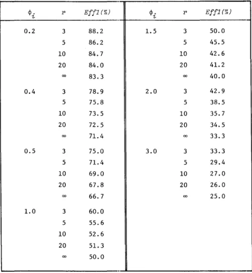
Eff1

var6 .)/Var6.)

'Z-

'Z-1/U

+

{l-l/r)<p.}

'Z-Table 4.1 shows the efficiency values so obtained, for the case r=3,5,10,20,00, as regards the parameter <p.=0.2, O.~l, 0.5,1.0,1.5,2.0,3.0.

'Z- These values

show that the efficiency is above 50 percent for all the values of rwhen <p. 'Z-is less than or equal to 1.

is below 50 percent.

However, if <p. is greater than 1, the efficiency

'Z-A

The estimate Ai is not so efficient as Ai when

<Pi

is greater than 1, since r. the number of the observed failures for the ith component decreases with

'Z-increasing <p .•

'Z- However, the time rE!quired for randomly censored life testing

A

Table 4.1 Efficiency of the Estimate A for A

r Eff1(%) 0.2 1.5 3 50.0 5 45.5 10 42.6 20 41.2 00 40.0 3 42.9 5 38.5 10 35.7 20 34.5 00 33.3 0.5 3.0 3 33.3 5 29.4 10 27.0 20 26.0 00 25.0 1.0

is less than that needed for theAith component life testing, because min(X

1,··

• ,X

k) ~ Xi. The efficiency of Ai will be investigated in the next section

considering both the variance of the estimate and the time required for life testing.

Remark 1.

(Another derivation of \.) It can be shown that the maximum

A ~A

likelihood estimate ~. of A. is given by ~.

=r./u

and this estimate is not

un-~ ~ ~ ~ ~ ~

biased (E(A.)=rA./(r-1)). The estimate

A.

is also derived changing A. into

~ ~ ~ ~

an unbiased estimate noting that {6.} and Z are independent.

~

Remark 2.

It may be unrealistic assuming that H(x) = xm, that is, the time-to-failure of each of the components in the system is Weibull distributed with the same shape parameter m. However, there are many cases in which the

unknown parameter

A.

must be infered conducting life test of the component when

~

m

is known. In this situation, Randomly censored life testing is recommended. The details are stated in the next section.

4.2 Time saving in random censorship

In order to plan an experiment in which individual components are observed until failure we need to consider not only sample size but also test time. If we insist on observing all individuals until failure we may need to wait un-acceptably. If, however, we are willing to accept a randomly censored life testing we may save a large proportion of the time until the last failure.

Let X

1j(j=1, ... ,n) be the survival time for the jth prototype of the

com-ponent having a distribution function F/X) = 1-exp{-A

1H(x)

L

The period of observation for the jth prototype will typically be limited by an ammount X

2j.

Formally speaking, the X

1j is censored on the right by the X2j since one

ob-serves only 1 {

o

if

X1j~

x

_2j

if

X_1j> X_2j where 6

1j indicates whether X1j is censored (61j= 0) or not (61j= 1). Under

the randolli censorship model the censoring variable X

2j is also assumed to be a

random sample, drawn independently of the X

1j, from a distribution F2(x)

=

1-exp{-A

2H(x)}. For the Z's, it is assumed that we observe r ordered values with Type IT censoring at r out of n: that is,

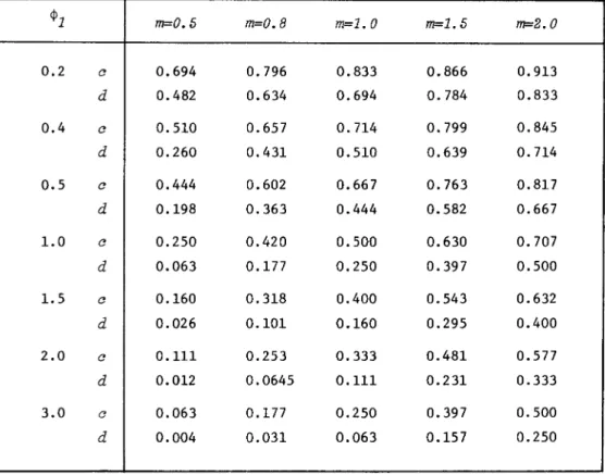
Zl < z2 < ••• < zr The ratio c=

E(z )/E(x

1 ) is the proportion of expected time we must wait

r r

fol-lowing way: c E(z ) r E(x 1r)

Statistical Analysis of Randomly Censored Data

n(n-l

)f

ooXAH ' (x)e-AH(x) U-e ->..H(x) )r-l (e -AH(x) )n-r dx

r-l 0 ne;:;) [XA

1H' (x)e -A1H(x) (1-e -A1H(x) )r-l (e -A1H(x) )n-r dx o

r:

H-1 (x/A)e -x (l-e -x )r-l (e-x )n-r dx

(H- 1 (x/A 1)e -x {1-e -x)r-l (e -x)n-r dx where 1..= 1..1 + 1.. 2. m Thus, if H(x) =X , we obtain c (A /A)l/m 1

since H-1 (x) = xl/m. The quantity 0/1..) < 1 shows that the time saving in-crease with decreasing

m.

Furthermore, the comparison of t::J.e variance of test time says that the variance of that for random censoring can be reduced, that is,

d = Var(z )/Var(x 1 ) < 1 r r I f H(x)

=

xm , d is given by d = (1+4> ;-2/m 1 199

m=0.5, 0.8,1.0,1.5,2.0 are presented in Table 4.2. Table 4.2 shoTMS that c and d decrease for fixed

m

as the value of 4>1 increases. Especially ran-domly censored life testing can reduce the variance of test time comparing Type

rr

censoring very much.

The result above shows that, for the purpose of comparing the random cen-soring with Type

rr

censoring, it is necessary to take both the variance of the estimate for 1..1 and the mean test tim'~ into consideration, espesially in the area of reliability theory. Conside-.cing both them, the efficiency for com-parison of the two life testing methods may be defined as

var-1

6

1)

1

-Eff2

/

Var (Al~.

E(z ) E(x

1)

,

which denotes the ratio of the information per unit time obtained for random censoring and that for Type

n

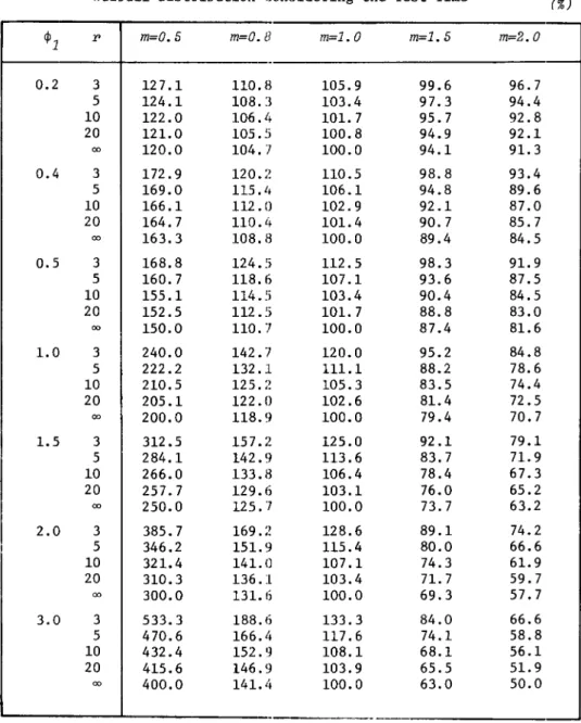
censoring.

If H (x) = xm, tha t is, Xl' s and X 2' s are Weibu11 dis tribu ted wi th the same shape parameter m, then Eff2 is given by

Eff2

=

(l+~l)l/m/{l+(l-l/r)$l}

Table 4.3 gives the numerical results of the calculations of Eff2 for $1=0.2,

0.4,0.5,1.0,1.5,2.0,3.0, for r=3, 5, 10, 20.,00, and for m=0.5, 0.8, 1.0,

1.5, 2.0. The numerical results show that Random censoring gives much more information per unit time than Type

n

censoring when m 2, 1 and the relative ef-ficiency increases with decreasing m and P. Hence it may be said that Random censoring can be used in place of Type

n

censoring when the time required for life testing is limited.

$1 0.2 0.4 0.5 1.0 1.5 2.0 3.0

Table 4.2 Ratios of the Mean and the Variance of the Relative WaLting Time for Weibu11 Distribution with the Shape Parameter m and Various Choices of $1 and m

rn=0.5 m=O.B m=1.0 m=1.5 rn=2.0 c 0.694 0.796 0.833 0.866 0.913 d 0.482 0.634 0.694 0.784 0.833 c 0.510 0.657 0.714 0.799 0.845 d 0.260 0.431 0.510 0.639 0.714 c 0.444 0.602 0.667 0.763 0.817 d 0.198 0.363 0.444 0.582 0.667 c 0.250 0.420 0.500 0.630 0.707 d 0.063 0.177 0.250 0.397 0.500 c 0.160 0.318 0.400 0.543 0.632 d 0.026 0.101 0.160 0.295 0.400 c 0.111 0.253 0.333 0.481 0.577 d 0.012 0.0645 0.111 0.231 0.333 c 0.063 0.177 0.250 0.397 0.500 d 0.004 0.031 0.063 0.157 0.250

Statistical Analysis of Randomly Censored Data 201

Finally, it is important that the choice of the parameter A2 must be done taking both the variance of the estimate and the time needed for life testing into consideration.

Remark. The result that Eff2~.1 when H(x) =xm and m2, 1 can be shown in the following way. Let

m~

1, then (1+4>l)l/m

~

1+4>1' Therefore,

A _

Table 4.3 Efficiency of the Estimate A for A for

Weibu11 Distribution Considering the Test Time _(%)

4>1 r m=O.5 m=O.B m=1.0 m=1.5 m=2.0

-0.2 3 127.1 110.8 105.9 99.6 96.7 5 124.1 108.3 103.4 97.3 94.4 10 122.0 106./1 101. 7 95.7 92.8 20 121.0 105.5 100.8 94.9 92.1 00 120.0 104.7 100.0 94.1 91. 3 0.4 3 172.9 120.2 110.5 98.8 93.4 5 169.0 115.il 106.1 94.8 89.6 10 166.1 112.0 102.9 92.1 87.0 20 164.7 110./1 101.4 90.7 85.7 00 163.3 108.8 100.0 _89.4 84.5 0.5 3 168.8 124. ~i 112.5 98.3 91. 9 5 160.7 118.6 107.1 93.6 87.5 10 155.1 114.5 103.4 90.4 84.5 20 152.5 112.5 101. 7 88.8 83.0 00 150.0 110.7 100.0 87.4 81.6 1.0 3 240.0 142.7 120.0 95.2 84.8 5 222.2 132.1 111.1 88.2 78.6 10 210.5 125.2 105.3 83.5 74.4 20 205.1 122.0 102.6 81.4 72 .5 00 200.0 118.9 100.0 79.4 70.7 1.5 3 312.5 157.2 125.0 92.1 79.1 5 284.1 142.9 113.6 83.7 71.9 10 266.0 133.8 106.4 78.4 67.3 20 257.7 129.6 103.1 76.0 65.2 00 250.0 125.7 100.0 73.7 63.2 2.0 3 385.7 169.2 128.6 89.1 74.2 5 346.2 151.9 115.4 80.0 66.6 10 321.4 141.0 107.1 74.3 61. 9 20 310.3 136.1 103.4 71. 7 59.7 00 300.0 131. I) 100.0 69.3 57.7 3.0 3 533.3 188.6 133.3 84.0 66.6 5 470.6 166. /1 117.6 74.1 58.8 10 432.4 152.9 108.1 68.1 56.1 20 415.6 146.9 103.9 65.5 51. 9 00 400.0 141. /1 100.0 63.0 50.0

-

-Eff2 (1+4>1) l/m 1+(1-1/r)4>1

5. Related Works

>

- - - = - - -

1+4>1 > 1 1+(1-1/r)4>1

Under random censorship Kaplan and Meier[5] give the product-limit (PL) estimate and reduced-sample (RS) estimate for the proportion P(t) of items in the population whose lifetimes would exceed t, without making any assumption about the form of the function P(t). PL estimate is the distribution, unre-stricted as to form, which maximizes the likelihood of the observations. Breslow and Crowley[3] give a necessary and sufficient condition for the con-sistency of the standard (actuarial) life table estimate of P(t) and asymptotic normality of this estimate, using the model of random censorship. Abe[l] giv-es a non-parametric giv-estimate for the life time distribution from observations of an aggregate of renewal processes.

determined by

Since the life time

Xo

of each unit is

where Xl and X₂ are mutually independent random variables with continuous dis-tribution functions, Abe's model is considered as one of the random censorship models.

Elveback[4] discusses a simple frequency estimate assuming that the sur-vivorship function is approximated by the polygonal function and shows that the method proposed is appropriate and highly efficient for large scale follow-up studies. Yang[7] deals with estimation of life expectancy used in survival analysis and competing risk study under the condition that the data are random-ly censored by

k

independent censoring variables and shows that the estimate converges weakly to a Gaussian process.

Muenz and Green[6] studies time savings in Type II censored life testing. Their measure of time savings is t(r)/t(n) which is the proportion of time we must wait if failures r+l through to n are not observed. They give numerical results and outline the application of this approach to the evaluation of early stopping procedures.

Acknowledgement.

The author wishes to thank Professor Hajime Makabe. Tokyo Institute of Technology, for his guidance and encouragement.

Statistical Analysis of Randomly Censored Data

References

[1] Abe. S.: Statistical Analysis of Reliability Data in Renewal Processes. Ann. Inst. Stat. Math., Vol. 23 (1970). 297-320.

[2] Berman. S. M.: Note on Extreme Values. Competing Risks and Semi-Markov Processes. Ann. Math. Stat., Vol. 34 (1963). 1104-1106.

203

[3] Breslow. N. and Crowley. J.: A Large Sample Study of the Life Table and Product Limit Estimates under F~ndom Censorship. Ann. Stat., Vol. 2 (1974). 437-453.

[4] Elveback. L.: Estimation of Survivorship in Chronic Disease: the "Actu-arial" Method. J. Ame1'. Stat. A880C., Vol. 53 (1958). 420-440.

[5] Kaplan. E. L. and Meier. P.: Nonparametric Estimation from Incomplete Observations. J. Ame1'. Stat. AS8oc., Vol. 53 (1958).457-481.

[6] Muenz. L. R. and Green. S. B.: Time Savings in Censored Life Test:lng.

J.

Roy. Stat. Soc., Vol. 39 (1977). 269-275.

[7] Yang. G.: Life Expectancy under Random Censorship. Stoch. Proc. AppZ., Vol. 6 (1977). 33-39.

A

Appendix. Derivation of the Variance of

Ai.

A

Noting that the random variables 1'. and u are independent. the variance

'Z-of

A.

is computed as the fllowing way:

'Z-Var(L)

'Z-Ai

2

2

~( l-A./A) +1' rAjA} 2 2 'Z- 2 " {1/(1'-2J+l}A - \ l ' 2 2 (1'-1) {1+((A-L}/A.) (1/1')}L /(1'-2) - L 'Z- 'Z- 'Z- 'Z-~ 2 (1'-1) (l+<p./1'}Var(A.) - A. 'Z- 1,

'Z-Tetsuo MIYAMURA: Department of Information Engineering. Faculty of Engineering. Ibaraki University. Nakanarusawa. Hitachi. Ibaraki 316. Japan