新潟の里雪・山雪と東アジア域での
ブロッキングと寒気流出経路
1
/25
*山崎哲(
JAMSTEC)
本田明治(新潟大学・自然科学)
川瀬宏明(気象研究所)
2016年2月16日「波と平均流の相互作用に関する研究会」
1. 寒気質量fluxを使って最近やっていること
2. アンサンブル再解析の紹介
最近やっていること
• 日本での降雪とブロッキングとの関係を
調べている.
– 現在は新潟の里雪・山雪との関係.
– 地域降水データから大循環場を復元(グロー
バル
=>ローカル).
• 東アジアや北米東岸域での寒気流出とブ
ロッキングとの関係について調べたい.
2
基本的な戦略
• グローバルな力学場を分析する.
– グローバルな変数(
u,v,T,z,Ps,…)を利用.
• だいたいは対流圏上層と下層の
2つだけを見る.
– 上層:
Z, EKE,…
– 下層:
T, v’T’,…
• (できれば)保存量で議論したい:
– 対流圏上層は
rich?: PV, Wave activity flux (WAF).
– 対流圏下層は少ない:θ
(flux)くらい?
4
Cold air mass (CAM) flux
(Iwasaki et al. 2014, JAS)and the western North Atlantic Ocean. Both disap-pearance regions have sharp line structures rising from 308N at the coasts to higher latitudes at their eastern ends. This reflects the sea surface temperature (SST) under a possible influence of the western boundary currents and their extensions. The cold air mass rapidly disappears at a maximal rate of about 100 hPa day21 owing to strong diabatic heating soon after it crosses a line of the SST of 280 K southward. Particularly in the Atlantic Ocean, the loss region of cold air mass reaches around 608N, where the Gulf Stream transports a large amount of ocean heat content northward and releases it to the atmosphere in higher latitudes (Minobe et al. 2008).
The mass flux can be decomposed into divergent/ irrotational and rotational/nondivergent components, as shown in Figs. 4c and 4d,
[pv] [ ðps
p(uT)
v dp 5 [pv]x 1 [pv]c, (10)
where the divergent and rotational components can be written in terms of scalar functions and the vertical unit vector k,
[pv]x 5 $x and [pv]c 5 2k 3 $c. (11)
The rotational component may present perpetual mo-tions that are not directly related to the diabatic change in the cold air mass. The divergent component primarily explains the temporal change in the geographical dis-tribution of the cold airmass amount as is expected from Eq. (3). Note that only the divergent component con-tributes to the mean meridional circulation in MIM as shown in Fig. 2. Roughly speaking, the magnitude of
FIG. 4. Geographical distributions of (a) cold airmass amount (hPa) and its horizontal flux with arrows, (b) genesis/
loss of cold air mass (hPa day21) with the SST line of 280 K, (c) divergent/irrotational component of cold airmass flux (hPa m s21), and (d) rotational/nondivergent component of cold airmass flux for DJF means over 1980/81–2009/10. Contour lines indicate topography with intervals of 500 m.
2234 J O U R N A L O F T H E A T M O S P H E R I C S C I E N C E S VOLUME 71
flow. In the MIM’s zonal mean, the lower-tropospheric equatorward flow is driven through wave–mean flow in-teractions (e.g., IM12). The Coriolis force of the equa-torward flow is almost in balance with Eliassen–Palm (E–P) flux divergence (Juckes et al. 1994; Tanaka et al. 2004; IM12). It indicates that long and ultralong waves play important roles in the formation of the equator-ward flow. This is somewhat similar to the extratropical pumping, which is well known as a major driving force of the stratospheric mean meridional circulation (e.g.,
Holton et al. 1995). In this work, the idea of the
ex-tratropical pumping is extended to the localized cold stream in the lower troposphere, with particular at-tention on the lower boundary conditions.
Many studies have been done on the polar cold air outbreaks frequently causing extreme cold events in mid- and low latitudes, especially around eastern North America (e.g., Dallavalle and Bosart 1975) and East Asia (e.g., Chang et al. 1979). Intermittent cold air outbreaks are accompanied by synoptic traveling dis-turbances in midlatitudes (e.g., Joung and Hitchman
1982; Lau and Lau 1984). The geographical features
of outbreaks are associated with the downstream de-velopment of synoptic disturbances from high moun-tains under control of quasi-stationary ultralong waves. The activity of quasi-stationary ultralong waves induces intraseasonal and interannual variations of cold air outbreaks (e.g., Boyle 1986; Schultz et al. 1998; Takaya
and Nakamura 2005; Jeong and Ho 2005; Park et al.
2011). In isobaric coordinates, however, the time-mean wind hardly indicates the cold airmass flux, because it includes warm winds. Therefore, previous studies treated the cold air outbreaks as anomalous events de-viated from the normal climate. Direct estimates, how-ever, have not been made of the stationary component of polar cold airmass flux yet.
Isentropic coordinates are convenient to trace the airmass trajectory. Harada (1962) studied the rapid ad-vancement of the head of cold air outbreak around Ja-pan in isentropic coordinates. Most isentropic analyses dealt with single-level synoptic charts subjectively, but did not deal with mass and heat balances quantitatively. The mass weighting introduced to MIM leads us to simple expressions of conservations of air mass and thermody-namic energy. The purpose of this study is to develop a quantitative diagnosis tool for the geographical distri-butions of polar cold airstreams in isentropic coordinates, which estimates its genesis/loss rates of a cold air mass based on conservations of the cold air mass and the neg-ative heat content. A preliminary analysis is made on the Northern Hemispheric winter climate of the polar cold airstreams, negative heat flows, and their diabatic genesis/ loss. Particular attention is paid to the stationary component
of polar cold airmass streams. Data used are the atmo-spheric reanalysis from the Japanese 25-year Reanalysis Project (JRA-25), conducted at the Japan Meteorolog-ical Agency (Onogi et al. 2007).
2. Conservation relations of polar cold air mass
and negative heat content
In this analysis, one of the key parameters in identi-fying the polar cold air mass is the threshold potential temperature uT. In MIM analyses, the potential
tem-perature at the turning point of the ETD circulation from the downward to the equatorward seems to be appropriate as a threshold value of the polar cold air mass, because the downward motion indicates the for-mation of the cold air mass and the equatorward motion reduces temperature owing to the horizontal advection in isentropic coordinates (IM12). Of course, the choice of uT is still open and impacts of modified
thresh-old temperatures will be discussed in section 5.
We first derive the governing equation of geo-graphical distribution of the cold air mass below the threshold potential temperature. Symbols are listed in
appendix B. At each grid point on the sphere, the total
cold airmass amount below uT is given by the pressure
difference between the ground surface and the isentro-pic surface of uT,
DP[ pS 2 p(uT) . (1) The isentropic mass continuity equation (see, e.g.,
Johnson 1980) can be written as
› ›t ! ›p ›u " 1 $ ! ! ›p ›u v " 1 › ›u ! ›p ›u _u " 5 0. (2)
The vertical integration of Eq. (2) from the lower boundary us to uT leads us to the total cold airmass conservation equation › ›tDP5 2$ ! ðps p(uT) v dp 1 G(uT) . (3)
The total cold airmass amount changes as a result of horizontal convergence and the vertical mass flux at uT.
The vertical mass flux crossing the uT surface G(uT) is related to the diabatic heating/cooling at uT,
G(uT) [ ›p ›u _u $ $ $ $ uT , (4)
where the diabatic cooling is the source of the cold air mass. Here G(uT) becomes negative when the cold air
JUNE 2014 I W A S A K I E T A L .
2231
flow. In the MIM’s zonal mean, the lower-tropospheric equatorward flow is driven through wave–mean flow in-teractions (e.g., IM12). The Coriolis force of the equa-torward flow is almost in balance with Eliassen–Palm (E–P) flux divergence (Juckes et al. 1994; Tanaka et al. 2004; IM12). It indicates that long and ultralong waves play important roles in the formation of the equator-ward flow. This is somewhat similar to the extratropical pumping, which is well known as a major driving force of the stratospheric mean meridional circulation (e.g.,
Holton et al. 1995). In this work, the idea of the ex-tratropical pumping is extended to the localized cold stream in the lower troposphere, with particular at-tention on the lower boundary conditions.
Many studies have been done on the polar cold air outbreaks frequently causing extreme cold events in mid- and low latitudes, especially around eastern North America (e.g., Dallavalle and Bosart 1975) and East Asia (e.g., Chang et al. 1979). Intermittent cold air outbreaks are accompanied by synoptic traveling dis-turbances in midlatitudes (e.g., Joung and Hitchman 1982; Lau and Lau 1984). The geographical features of outbreaks are associated with the downstream de-velopment of synoptic disturbances from high moun-tains under control of quasi-stationary ultralong waves. The activity of quasi-stationary ultralong waves induces intraseasonal and interannual variations of cold air outbreaks (e.g., Boyle 1986; Schultz et al. 1998; Takaya and Nakamura 2005; Jeong and Ho 2005; Park et al. 2011). In isobaric coordinates, however, the time-mean wind hardly indicates the cold airmass flux, because it includes warm winds. Therefore, previous studies treated the cold air outbreaks as anomalous events de-viated from the normal climate. Direct estimates, how-ever, have not been made of the stationary component of polar cold airmass flux yet.
Isentropic coordinates are convenient to trace the airmass trajectory. Harada (1962) studied the rapid ad-vancement of the head of cold air outbreak around Ja-pan in isentropic coordinates. Most isentropic analyses dealt with single-level synoptic charts subjectively, but did not deal with mass and heat balances quantitatively. The mass weighting introduced to MIM leads us to simple expressions of conservations of air mass and thermody-namic energy. The purpose of this study is to develop a quantitative diagnosis tool for the geographical distri-butions of polar cold airstreams in isentropic coordinates, which estimates its genesis/loss rates of a cold air mass based on conservations of the cold air mass and the neg-ative heat content. A preliminary analysis is made on the Northern Hemispheric winter climate of the polar cold airstreams, negative heat flows, and their diabatic genesis/ loss. Particular attention is paid to the stationary component
of polar cold airmass streams. Data used are the atmo-spheric reanalysis from the Japanese 25-year Reanalysis Project (JRA-25), conducted at the Japan Meteorolog-ical Agency (Onogi et al. 2007).
2. Conservation relations of polar cold air mass and negative heat content
In this analysis, one of the key parameters in identi-fying the polar cold air mass is the threshold potential temperature uT. In MIM analyses, the potential tem-perature at the turning point of the ETD circulation from the downward to the equatorward seems to be appropriate as a threshold value of the polar cold air mass, because the downward motion indicates the for-mation of the cold air mass and the equatorward motion reduces temperature owing to the horizontal advection in isentropic coordinates (IM12). Of course, the choice of uT is still open and impacts of modified thresh-old temperatures will be discussed in section 5.
We first derive the governing equation of geo-graphical distribution of the cold air mass below the threshold potential temperature. Symbols are listed in
appendix B. At each grid point on the sphere, the total cold airmass amount below uT is given by the pressure difference between the ground surface and the isentro-pic surface of uT,
DP[ pS 2 p(uT) . (1)
The isentropic mass continuity equation (see, e.g.,
Johnson 1980) can be written as › ›t ! ›p ›u " 1 $ ! ! ›p ›u v " 1 › ›u ! ›p ›u _u " 5 0. (2)
The vertical integration of Eq. (2) from the lower boundary us to uT leads us to the total cold airmass conservation equation › ›tDP5 2$ ! ðps p(uT) v dp 1 G(uT) . (3)
The total cold airmass amount changes as a result of horizontal convergence and the vertical mass flux at uT. The vertical mass flux crossing the uT surface G(uT) is related to the diabatic heating/cooling at uT,
G(uT) [›p ›u _u $ $ $ $ uT , (4)
where the diabatic cooling is the source of the cold air mass. Here G(uT) becomes negative when the cold air
JUNE 2014 I W A S A K I E T A L . 2231
flow. In the MIM’s zonal mean, the lower-tropospheric equatorward flow is driven through wave–mean flow in-teractions (e.g., IM12). The Coriolis force of the equa-torward flow is almost in balance with Eliassen–Palm (E–P) flux divergence (Juckes et al. 1994; Tanaka et al. 2004; IM12). It indicates that long and ultralong waves play important roles in the formation of the equator-ward flow. This is somewhat similar to the extratropical pumping, which is well known as a major driving force of the stratospheric mean meridional circulation (e.g.,
Holton et al. 1995). In this work, the idea of the
ex-tratropical pumping is extended to the localized cold stream in the lower troposphere, with particular at-tention on the lower boundary conditions.
Many studies have been done on the polar cold air outbreaks frequently causing extreme cold events in mid- and low latitudes, especially around eastern North America (e.g., Dallavalle and Bosart 1975) and East Asia (e.g., Chang et al. 1979). Intermittent cold air outbreaks are accompanied by synoptic traveling dis-turbances in midlatitudes (e.g., Joung and Hitchman
1982; Lau and Lau 1984). The geographical features
of outbreaks are associated with the downstream de-velopment of synoptic disturbances from high moun-tains under control of quasi-stationary ultralong waves. The activity of quasi-stationary ultralong waves induces intraseasonal and interannual variations of cold air outbreaks (e.g., Boyle 1986; Schultz et al. 1998; Takaya
and Nakamura 2005; Jeong and Ho 2005; Park et al.
2011). In isobaric coordinates, however, the time-mean wind hardly indicates the cold airmass flux, because it includes warm winds. Therefore, previous studies treated the cold air outbreaks as anomalous events de-viated from the normal climate. Direct estimates, how-ever, have not been made of the stationary component of polar cold airmass flux yet.
Isentropic coordinates are convenient to trace the airmass trajectory. Harada (1962) studied the rapid ad-vancement of the head of cold air outbreak around Ja-pan in isentropic coordinates. Most isentropic analyses dealt with single-level synoptic charts subjectively, but did not deal with mass and heat balances quantitatively. The mass weighting introduced to MIM leads us to simple expressions of conservations of air mass and thermody-namic energy. The purpose of this study is to develop a quantitative diagnosis tool for the geographical distri-butions of polar cold airstreams in isentropic coordinates, which estimates its genesis/loss rates of a cold air mass based on conservations of the cold air mass and the neg-ative heat content. A preliminary analysis is made on the Northern Hemispheric winter climate of the polar cold airstreams, negative heat flows, and their diabatic genesis/ loss. Particular attention is paid to the stationary component
of polar cold airmass streams. Data used are the atmo-spheric reanalysis from the Japanese 25-year Reanalysis Project (JRA-25), conducted at the Japan Meteorolog-ical Agency (Onogi et al. 2007).
2. Conservation relations of polar cold air mass and negative heat content
In this analysis, one of the key parameters in identi-fying the polar cold air mass is the threshold potential temperature uT. In MIM analyses, the potential
tem-perature at the turning point of the ETD circulation from the downward to the equatorward seems to be appropriate as a threshold value of the polar cold air mass, because the downward motion indicates the for-mation of the cold air mass and the equatorward motion reduces temperature owing to the horizontal advection in isentropic coordinates (IM12). Of course, the choice of uT is still open and impacts of modified
thresh-old temperatures will be discussed in section 5.
We first derive the governing equation of geo-graphical distribution of the cold air mass below the threshold potential temperature. Symbols are listed in
appendix B. At each grid point on the sphere, the total
cold airmass amount below uT is given by the pressure
difference between the ground surface and the isentro-pic surface of uT,
DP[ pS 2 p(uT) . (1) The isentropic mass continuity equation (see, e.g.,
Johnson 1980) can be written as
› ›t ! ›p ›u " 1 $ ! ! ›p ›uv " 1 › ›u ! ›p ›u _u " 5 0. (2) The vertical integration of Eq. (2) from the lower boundary us to uT leads us to the total cold airmass
conservation equation › ›t DP5 2$ ! ðps p(uT) v dp 1 G(uT) . (3) The total cold airmass amount changes as a result of horizontal convergence and the vertical mass flux at uT. The vertical mass flux crossing the uT surface G(uT) is
related to the diabatic heating/cooling at uT,
G(uT) [›p ›u _u $ $ $ $ uT , (4) where the diabatic cooling is the source of the cold air mass. Here G(uT) becomes negative when the cold air
JUNE 2014 I W A S A K I E T A L . 2231
flow. In the MIM’s zonal mean, the lower-tropospheric equatorward flow is driven through wave–mean flow in-teractions (e.g., IM12). The Coriolis force of the equa-torward flow is almost in balance with Eliassen–Palm (E–P) flux divergence (Juckes et al. 1994; Tanaka et al. 2004; IM12). It indicates that long and ultralong waves play important roles in the formation of the equator-ward flow. This is somewhat similar to the extratropical pumping, which is well known as a major driving force of the stratospheric mean meridional circulation (e.g.,
Holton et al. 1995). In this work, the idea of the
ex-tratropical pumping is extended to the localized cold stream in the lower troposphere, with particular at-tention on the lower boundary conditions.
Many studies have been done on the polar cold air outbreaks frequently causing extreme cold events in mid- and low latitudes, especially around eastern North America (e.g., Dallavalle and Bosart 1975) and East Asia (e.g., Chang et al. 1979). Intermittent cold air outbreaks are accompanied by synoptic traveling dis-turbances in midlatitudes (e.g., Joung and Hitchman
1982; Lau and Lau 1984). The geographical features
of outbreaks are associated with the downstream de-velopment of synoptic disturbances from high moun-tains under control of quasi-stationary ultralong waves. The activity of quasi-stationary ultralong waves induces intraseasonal and interannual variations of cold air outbreaks (e.g., Boyle 1986; Schultz et al. 1998; Takaya
and Nakamura 2005; Jeong and Ho 2005; Park et al.
2011). In isobaric coordinates, however, the time-mean wind hardly indicates the cold airmass flux, because it includes warm winds. Therefore, previous studies treated the cold air outbreaks as anomalous events de-viated from the normal climate. Direct estimates, how-ever, have not been made of the stationary component of polar cold airmass flux yet.
Isentropic coordinates are convenient to trace the airmass trajectory. Harada (1962) studied the rapid ad-vancement of the head of cold air outbreak around Ja-pan in isentropic coordinates. Most isentropic analyses dealt with single-level synoptic charts subjectively, but did not deal with mass and heat balances quantitatively. The mass weighting introduced to MIM leads us to simple expressions of conservations of air mass and thermody-namic energy. The purpose of this study is to develop a quantitative diagnosis tool for the geographical distri-butions of polar cold airstreams in isentropic coordinates, which estimates its genesis/loss rates of a cold air mass based on conservations of the cold air mass and the neg-ative heat content. A preliminary analysis is made on the Northern Hemispheric winter climate of the polar cold airstreams, negative heat flows, and their diabatic genesis/ loss. Particular attention is paid to the stationary component
of polar cold airmass streams. Data used are the atmo-spheric reanalysis from the Japanese 25-year Reanalysis Project (JRA-25), conducted at the Japan Meteorolog-ical Agency (Onogi et al. 2007).
2. Conservation relations of polar cold air mass
and negative heat content
In this analysis, one of the key parameters in identi-fying the polar cold air mass is the threshold potential temperature uT. In MIM analyses, the potential
tem-perature at the turning point of the ETD circulation from the downward to the equatorward seems to be appropriate as a threshold value of the polar cold air mass, because the downward motion indicates the for-mation of the cold air mass and the equatorward motion reduces temperature owing to the horizontal advection in isentropic coordinates (IM12). Of course, the choice of uT is still open and impacts of modified
thresh-old temperatures will be discussed in section 5.
We first derive the governing equation of geo-graphical distribution of the cold air mass below the threshold potential temperature. Symbols are listed in
appendix B. At each grid point on the sphere, the total
cold airmass amount below uT is given by the pressure
difference between the ground surface and the isentro-pic surface of uT,
DP[ pS 2 p(uT) . (1) The isentropic mass continuity equation (see, e.g.,
Johnson 1980) can be written as
› ›t ! ›p ›u " 1 $ ! ! ›p ›uv " 1 › ›u ! ›p ›u _u " 5 0. (2) The vertical integration of Eq. (2) from the lower boundary us to uT leads us to the total cold airmass
conservation equation › ›tDP5 2$ ! ðps p(uT) v dp 1 G(uT) . (3) The total cold airmass amount changes as a result of horizontal convergence and the vertical mass flux at uT.
The vertical mass flux crossing the uT surface G(uT) is
related to the diabatic heating/cooling at uT,
G(uT) [›p ›u _u $ $ $ $ uT , (4) where the diabatic cooling is the source of the cold air mass. Here G(uT) becomes negative when the cold air
JUNE 2014 I W A S A K I E T A L .
2231
equatorward at around 458N, and causes the descending adiabatic heating north of 458N and the advective cooling south of 458N (IM12). The latitude of 458N is regarded as the turning latitude in isentropic co-ordinates. In the ETD circulation, the equatorward flow is almost confined below about isentropic zonal mean pressure of 850 hPa. Thus, the potential temperature of about 280 K at the point (458N, 850 hPa) is set to be the threshold uT in this work. The choice of uT is still
changeable depending on research purposes. The sen-sitivity to uT is examined insection 5briefly.
b. Cold air dome
Figure 3 plots the geographical distribution of the geopotential height at uT 5 280 K averaging over DJF
during 1981–2010. This looks like a cold air dome in the Northern Hemispheric winter and is regarded as the reservoir of cold air mass flowing out to lower latitudes. It reaches almost 5000 m high near the North Pole. The cold dome elongates from eastern Siberia to the Hudson Bay. These two ridges of the cold dome correspond to thermal stationary troughs in the middle-tropospheric isobaric surfaces. The isentropic surface is very steep near the ends of the two ridges around East Asia and the eastern coast of North America, indicating large baro-clinicity. The third ridge is located around eastern Europe with much smaller amplitude than the two major ridges.
As is well known, distinct storm tracks are formed in the western North Pacific Ocean and western North Atlantic Ocean (Wallace et al. 1988;Hoskins and Valdes
1990). The large baroclinicity has been recognized to be a major reason for the formation of storm tracks. Isen-tropic geopotential heights are found to have large gradients near the storm tracks. Gradients of isentropic geopotential heights indicate the magnitude of the baro-clinicity, since the downgradient mass flux releases a lot of the available potential energy.
The geopotential height of uT surface must be
com-pared with the topography. Over the Eurasian conti-nent, the isentropic geopotential height at uT is much
lower than the mountain ranges located from 308 to 408N. Thus, the polar cold air mass is confined on the polar side of the mountain ranges over the central Eur-asia, but it cannot cross equatorward over the mountain range.
c. Main streams of the polar cold air mass
Figure 4aillustrates the geographical distributions of the total cold airmass amount below uT 5 280 K and
their horizontal flux. The airmass amount is presented by the airmass thickness DP [ pS2 p(uT) from the
ground surface to the isentropic surface of uT 5 280 K.
The polar cold airmass amount increases with latitudes and reaches a maximum of about 500 hPa near the North Pole. A large amount of the cold air mass is located within the circumpolar vortex. Nevertheless, the thick-ness distribution of cold airmass amount significantly deviates from axial symmetry.
Figure 4bshows the diabatic genesis/loss rate of the polar cold air mass below uTin Eq.(4). The cold air mass
is generated at a rate of 10–50 hPa day21over the con-tinent and sea ice areas north of 458N, the northern part of Eurasian continent, the Arctic Ocean, and the northern part of North America. On the other hand, it mostly disappears over the western North Pacific Ocean
FIG. 2. Meridional cross sections of MIM’s mass streamfunctions (contour interval 1010kg s21) and potential temperature (contour
interval 10 K) for DJF means over 1980/81–2009/10. A black dot is placed at the turning point (see text) of 458N and isentropic zonal mean pressure of 850 hPa. The potential temperature is about 280 K at this point. Black colors indicate the zonally averaged topography.
FIG. 3. Geopotential height of isentropic surface of uT 5 280 K
for DJF means over 1980/81–2009/10. Contour lines indicate the topography with intervals of 500 m.
JUNE2014 I W A S A K I E T A L . 2233
Cold air mass
CAM flux
DP (CAM)
個人的見解
•
PVやWAFやCAM fluxは保存量に基づくの
で,寒気やエネルギーの起源を分析する
上で非常に有益.
•
WAFやCAM fluxは微分階数が少ないので
高次のノイズが減り総観規模の解析に向
いていると思う.
5
flow. In the MIM’s zonal mean, the lower-tropospheric equatorward flow is driven through wave–mean flow in-teractions (e.g., IM12). The Coriolis force of the equa-torward flow is almost in balance with Eliassen–Palm (E–P) flux divergence (Juckes et al. 1994; Tanaka et al. 2004; IM12). It indicates that long and ultralong waves play important roles in the formation of the equator-ward flow. This is somewhat similar to the extratropical pumping, which is well known as a major driving force of the stratospheric mean meridional circulation (e.g.,
Holton et al. 1995). In this work, the idea of the
ex-tratropical pumping is extended to the localized cold stream in the lower troposphere, with particular at-tention on the lower boundary conditions.
Many studies have been done on the polar cold air outbreaks frequently causing extreme cold events in mid- and low latitudes, especially around eastern North America (e.g., Dallavalle and Bosart 1975) and East Asia (e.g., Chang et al. 1979). Intermittent cold air outbreaks are accompanied by synoptic traveling dis-turbances in midlatitudes (e.g., Joung and Hitchman
1982; Lau and Lau 1984). The geographical features
of outbreaks are associated with the downstream de-velopment of synoptic disturbances from high moun-tains under control of quasi-stationary ultralong waves. The activity of quasi-stationary ultralong waves induces intraseasonal and interannual variations of cold air outbreaks (e.g., Boyle 1986; Schultz et al. 1998; Takaya
and Nakamura 2005; Jeong and Ho 2005; Park et al.
2011). In isobaric coordinates, however, the time-mean wind hardly indicates the cold airmass flux, because it includes warm winds. Therefore, previous studies treated the cold air outbreaks as anomalous events de-viated from the normal climate. Direct estimates, how-ever, have not been made of the stationary component of polar cold airmass flux yet.
Isentropic coordinates are convenient to trace the airmass trajectory. Harada (1962) studied the rapid ad-vancement of the head of cold air outbreak around Ja-pan in isentropic coordinates. Most isentropic analyses dealt with single-level synoptic charts subjectively, but did not deal with mass and heat balances quantitatively. The mass weighting introduced to MIM leads us to simple expressions of conservations of air mass and thermody-namic energy. The purpose of this study is to develop a quantitative diagnosis tool for the geographical distri-butions of polar cold airstreams in isentropic coordinates, which estimates its genesis/loss rates of a cold air mass based on conservations of the cold air mass and the neg-ative heat content. A preliminary analysis is made on the Northern Hemispheric winter climate of the polar cold airstreams, negative heat flows, and their diabatic genesis/ loss. Particular attention is paid to the stationary component
of polar cold airmass streams. Data used are the atmo-spheric reanalysis from the Japanese 25-year Reanalysis Project (JRA-25), conducted at the Japan Meteorolog-ical Agency (Onogi et al. 2007).
2. Conservation relations of polar cold air mass and negative heat content
In this analysis, one of the key parameters in identi-fying the polar cold air mass is the threshold potential temperature uT. In MIM analyses, the potential
tem-perature at the turning point of the ETD circulation from the downward to the equatorward seems to be appropriate as a threshold value of the polar cold air mass, because the downward motion indicates the for-mation of the cold air mass and the equatorward motion reduces temperature owing to the horizontal advection in isentropic coordinates (IM12). Of course, the choice of uT is still open and impacts of modified
thresh-old temperatures will be discussed in section 5.
We first derive the governing equation of geo-graphical distribution of the cold air mass below the threshold potential temperature. Symbols are listed in
appendix B. At each grid point on the sphere, the total
cold airmass amount below uT is given by the pressure
difference between the ground surface and the isentro-pic surface of uT,
DP [ pS 2 p(uT) . (1) The isentropic mass continuity equation (see, e.g.,
Johnson 1980) can be written as
› ›t ! ›p ›u " 1 $ ! ! ›p ›u v " 1 › ›u ! ›p ›u _u " 5 0. (2) The vertical integration of Eq. (2) from the lower boundary us to uT leads us to the total cold airmass conservation equation › ›tDP 5 2$ ! ðps p(uT) v dp 1 G(uT) . (3) The total cold airmass amount changes as a result of horizontal convergence and the vertical mass flux at uT. The vertical mass flux crossing the uT surface G(uT) is
related to the diabatic heating/cooling at uT,
G(uT) [›p ›u _u $ $ $ $ uT , (4) where the diabatic cooling is the source of the cold air mass. Here G(uT) becomes negative when the cold air
JUNE 2014 I W A S A K I E T A L . 2231
新潟での里雪・山雪
6
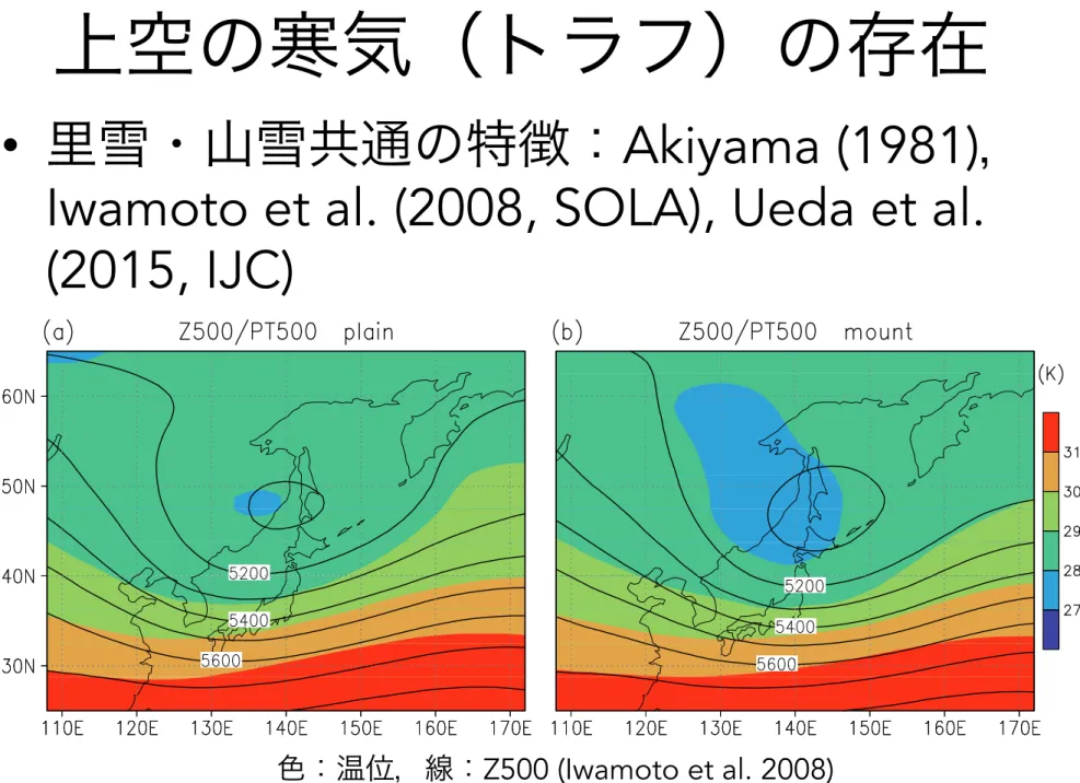
山域 里域 1月の最大積雪量(気象庁HPより) Akiyama (1981, JMSJ) 日本海 太平洋上空の寒気(トラフ)の存在
7
• 里雪・山雪共通の特徴:
Akiyama (1981),
Iwamoto et al. (2008, SOLA), Ueda et al.
(2015, IJC)
Iwamoto et al., Snowfall Distribution in the Niigata Area
wet-snow regions; that is, the average temperature in
winter is relatively high (Ishizaka 2004). In order to
avoid the inclusion of rainfall in the analysis, the cases
in which the daily-averaged temperature at 500 hPa at
the upper-air observation site, Wajima, was higher than
30
°C were removed from the analysis (the position of
Wajima is designated in the upper panel of Fig. 1). The
types of precipitation in Niigata are determined by the
spatial pattern of EOFs for the daily precipitation on a
correlation matrix. The component of the seasonal
evo-lution from December to February was removed by
sub-tracting the daily 19-year-average precipitation at each
station before calculating the correlation matrix. The
temporal variation of each precipitation type is
deter-mined by the time series of EOFs.
The daily winds observed at the weather stations of
AMeDAS were also used. The daily wind was calculated
by averaging the hourly wind over 24 hours with
respect to the zonal and meridional components. In
addition to these data, Japanese 25-year reanalysis
(JRA-25) with a horizontal resolution of 1.25
° × 1.25°
analyzed from 1979 to 2004, the JMA Climate Data
Assimilation System (JCDAS) after 2005 (Onogi et al.
2007), and the upper-air observation data at Wajima
were used as the reference data of the synoptic
condi-tions.
3. Precipitation types in Niigata
Figure 2 shows the spatial pattern of the leading and
secondary modes of EOFs (EOF1 and EOF2,
respec-tively), which account for nearly 70% of the total
variance up to EOF2. The positive value spreads
throughout the domain in EOF1. The values are
rela-tively low in the northern and southern parts of the
domain and reach a maximum at altitudes from 100 m
to 300 m between the lower-value areas. The time series
of EOF1 has positive correlations to the precipitation at
the northwestern slope of the mountainous backbone
not only in Niigata but also throughout Hokuriku
(Figure not shown). We assume that the EOF1
repre-sents the overall precipitation pattern associated with
the northwesterly winter monsoon. On the other hand,
EOF2 has a positive maximum in the plains and a
negative maximum in the mountains (Fig. 2b). The node
exists between the altitudes of 100 m and 300 m,
coin-ciding with the maximum area of EOF1. This pattern is
similar to the EOF2 represented by Akiyama (1981a).
Therefore, this mode is considered to characterize the
plain-type (positive phase, P-type) and the
mountain-type (negative phase, M-mountain-type) precipitation patterns. In
this study, the cases in which the daily time series of
EOF1 was 1.0 times larger than the standard deviation
(1.0!) were selected as the precipitation due to the
winter monsoon. In the selected cases, the precipitation
type was categorized as P-type when the daily time
series of EOF2 was larger than 1.0!and as M-type when
the time series was smaller than 1.0!.
4. Synoptic-scale structures with the
precipi-tation types
Figure 3 contains composite maps of the height and
the temperature fields at the occurrence of the P- and
M-type precipitation. With the P- and M-M-types, there are
upper troughs over the Sea of Japan and around the
Japan Islands, respectively, which are accompanied by
the cold air to the west (Figs. 3a and 3b). Consequently,
the P- and M-type precipitation occurs ahead of and
under the upper trough, respectively. Although the
potential temperature with the M-type is colder than
that with the P-type at the center of the cold air, the
temperatures do not show a significant difference in the
southwestern Sea of Japan. Corresponding to the upper
troughs, the lower trough extends from the Sea of
46
Fig. 2. Spatial patterns of (a) the leading EOF (EOF1) and (b) the
secondary EOF (EOF2). EOF is performed on the correlation
matrix. EOF1 and EOF2 account for 47.2% and 21.2% of the
total variance, respectively.
Fig. 3. Composite potential temperature (color) and height
(contour) of (a) P-type and (b) M-type at 500 hPa and the
poten-tial temperature difference between 500 hPa and 1,000 hPa
(color) and height at 925 hPa (contour) at the occurrence of (c)
P-type and (d) M-type.
Fig. 4. Composite vertical profiles of (a) wind direction, (b) wind
speed, and (c) equivalent potential temperature using the
upper-air observation data from 1988 to 2007 at Wajima. The
red and blue lines indicate the P- and M-types, respectively.
目的
8
• 里雪・山雪の要因となる日本上空のトラフの成
因は何か?
• 低周波変動と関係しているのか?特に
10日
(旬)スケールの変動に注目
– ブロッキングなどの振幅の大きな現象の時間スケー
ル.
– 多里雪・山雪時の旬(
10日間)で大循環場
(
JRA-55を利用)をコンポジットしてみる.
里雪・山雪イベント
の抽出
1. 里(山)域5 (6)地点の旬
降雪量データを気象庁よ
り取得.それぞれの域で
積算平均する.
2. 里,山域で旬別に降雪量
の平均と標準偏差を計算
(
1980/81∼2014/15年
の
DJF: 計315旬).
3. 各旬の降雪量を標準偏差
で割る
=>規格化降雪量.
4. 里や山域での規格化降雪
量トップ
15旬を抽出.
9
新潟(Niigata) 新津(Niitsu) 長岡(Nagaoka) 下関(Shimoseki) 津川(Tsugawa) 湯沢(Yuzawa) 関山(Sekiyama) 津南(Tsunan) 守門(Sumon) 十日町(Tohkamachi) 小出(Kode)10
「里雪」
「非山雪」
「山雪」 r = 0.73
10日平均合成図(top 15旬)
11
里雪 z250 非里雪 10日平均アノマリー(色)・気候値(コンター) 山雪 シベリア アリューシャンエネルギー伝播(波活動度
flux)
12
里雪 z250 非里雪 ベクトルは95%有意のみ 山雪 シベリア アリューシャン H westerly jet H LWave activity flux
北西太平洋
orシベリアでの
ブロッキング
?
13
1 MARCH 2003 P E L L Y A N D H O S K I N S 745
FIG. 1. Analyses of (a) 250-hPa geopotential height (dam) and (b)u(K) on PV 5 2 for 1200 UTC 21 Sep 1998.
FIG. 2. A schematic representation of the relevant parameters for
calculating the PV–ublocking index B at a given longitudel0. The
thick line is a representativeuon PV 5 2 contour during a blocking event centered atl0in this case.
associate blocking with a reversal of the normal negative meridional gradient in u on PV 5 2, and this forms the basis of the dynamical blocking index defined and used here.
a. Blocking index and local instantaneous blocking
Figure 2 shows a schematic representation of the rel-evant parameters used here for defining a blocking index
B at a given longitude l0. The thick line is a represen-tative u on PV 5 2 contour during a blocking episode, which is centered at l0 in this case.
The blocking indexB at longitude l0is defined as the difference in the average potential temperatures in the northern and southern boxes:
f 1Df / 20 f0
2 2
B 5
E
u df 2E
u df. (4)Df f Df f 2Df / 2
0 0
By this definition, B , 0 in the westerly flow over
Asia in Fig. 1, but B . 0 in the blocking regions over
Europe and western Canada. The longitude l0could be said to be blocked ifB . 0, indicating that there is high
potential temperature to the north and low potential tem-perature to the south.
As was noted above, Lejena¨s and Økland (1983), Ti-baldi and Molteni (1990), and D’Andrea et al. (1998) all used the same value, independent of longitude, for the central blocking latitude fc. However, if we return to a consideration of the fundamental nature of blocking, a different choice is suggested.
Since blocking is associated with the interruption of the midlatitude westerly jet and the blocking of mobile midlatitude weather systems, we could use either aspect to suggest the specification of fc. Using the westerly jet has problems associated with the subtropical jet. At some longitudes, for example in the European–North African sector, on average there are two jets. At other longitudes, for example in the western North Pacific, the weather systems are typically on the polar flank of the subtropical jet. Consequently, it is more convenient to use an average measure of weather system activity to define fc.
In order to represent the latitude–longitude distribu-tion of midlatitude weather systems, Fig. 3 shows the climatological annual mean high-pass transient eddy ki-netic energy (EKE) at 300 hPa. The Northern Hemi-sphere maxima in synoptic activity associated with the Atlantic and Pacific storm tracks are evident at around 408–508N. These latitudes are indeed representative of
1 MARCH2003 P E L L Y A N D H O S K I N S 745
FIG. 1. Analyses of (a) 250-hPa geopotential height (dam) and (b) u (K) on PV 5 2 for 1200 UTC 21 Sep 1998.
FIG. 2. A schematic representation of the relevant parameters for calculating the PV–u blocking indexB at a given longitude l0. The
thick line is a representative u on PV 5 2 contour during a blocking event centered at l0in this case.
associate blocking with a reversal of the normal negative meridional gradient in u on PV 5 2, and this forms the basis of the dynamical blocking index defined and used here.
a. Blocking index and local instantaneous blocking
Figure 2 shows a schematic representation of the rel-evant parameters used here for defining a blocking index
B at a given longitude l0. The thick line is a
represen-tative u on PV 5 2 contour during a blocking episode, which is centered at l0in this case.
The blocking indexB at longitude l0is defined as the
difference in the average potential temperatures in the northern and southern boxes:
f 1Df / 20 f0
2 2
B 5
E
u df 2E
u df. (4)Df f0 Df f 2Df / 20
By this definition, B , 0 in the westerly flow over
Asia in Fig. 1, butB . 0 in the blocking regions over
Europe and western Canada. The longitude l0could be
said to be blocked ifB . 0, indicating that there is high
potential temperature to the north and low potential tem-perature to the south.
As was noted above, Lejena¨s and Økland (1983), Ti-baldi and Molteni (1990), and D’Andrea et al. (1998) all used the same value, independent of longitude, for the central blocking latitude fc. However, if we return
to a consideration of the fundamental nature of blocking, a different choice is suggested.
Since blocking is associated with the interruption of the midlatitude westerly jet and the blocking of mobile midlatitude weather systems, we could use either aspect to suggest the specification of fc. Using the westerly
jet has problems associated with the subtropical jet. At some longitudes, for example in the European–North African sector, on average there are two jets. At other longitudes, for example in the western North Pacific, the weather systems are typically on the polar flank of the subtropical jet. Consequently, it is more convenient to use an average measure of weather system activity to define fc.
In order to represent the latitude–longitude distribu-tion of midlatitude weather systems, Fig. 3 shows the climatological annual mean high-pass transient eddy ki-netic energy (EKE) at 300 hPa. The Northern Hemi-sphere maxima in synoptic activity associated with the Atlantic and Pacific storm tracks are evident at around 408–508N. These latitudes are indeed representative of
Pelly and Hoskins (2003, JAS)
里雪
非里雪
120E
wave-train/ Pacific-origin type
14
are based on composite anomaly evolution for the 20 strongest upper-level blocking episodes, as shown in Fig. 1, for each of the grid points over the extratropical Eurasian continent and the northwestern Pacific. Fig-ure 5 shows clear geographical dependency of those two types of upper-level blocking formation, which ap-pears to be related to climatological features of the upper-tropospheric wintertime circulation. The wave-train (Atlantic-origin) type characterized by propaga-tion of a quasi-stapropaga-tionary Rossby wave packet over the Eurasian continent is found common over a vast area of central and western Siberia, located to the west of the climatological-mean trough over the Far East. At some locations, the main anticyclonic center associated with the wave-train (Atlantic-origin) type moves slowly east-ward, as shown in Fig. 1. The blocking formation of this type that occurs under modest feedback forcing from
transient eddies (Fig. 2) is thus primary through low-frequency dynamics associated with a propagating quasi-stationary Rossby waves, as pointed out by Na-kamura (1994), NaNa-kamura et al. (1997) and Swanson (2000). Meanwhile, the Pacific-origin type character-ized by slow retrogression of the primary anticyclonic center from the North Pacific region with no apparent signature of any incoming quasi-stationary wave packet (Fig. 3) is found common over eastern Siberia located to the east of the climatological trough. The retrogres-sion of anticyclonic anomalies, which may be related to the results of Kushnir (1987), Branstator (1987), and Lau and Nath (1999), occurs under strong feedback forcing from the Pacific storm track. A comparison be-tween Fig. 2 in TN05 and Fig. 5 reveals that, although blocking formation of the Pacific-origin type tends to be followed by a cold air outbreak to the midlatitude
FIG. 5. Geographical distribution of the wave-train (Atlantic-origin) and Pacific-origin types
on the basis of upper-level blocking composites over the Eurasian continent and the north-western Pacific Ocean. Each of the heavy lines signifies a propagation axis of a wave train at the 250-hPa level for the wave-train type. An end of the line with a closed triangle marks the position of a blocking ridge at its peak time, while the other end corresponds to the position of the strongest upstream cyclonic anomaly center associated with the wave train 4 days before the peak time. Each of the light lines signifies a migration path of the primary anticyclonic anomaly center at the 250-hPa level. An end of the line with a triangle corresponds to the anticyclonic center at its peak time, while the other end corresponds to the same center but 4 days before its peak time. Contour lines indicate the climatological-mean Ertel’s PV at the 330-K isentropic surface (contoured every 1 PVU from 2.5 PVU). The statistics shown in this figure are based on the 250-hPa composite anomaly evolution for the 20 strongest blocking events around each of the grid points over the Eurasian and northwestern Pacific regions, but those only for selected grid points are shown for clarity. The wave-train (Atlantic-origin) type is characterized by an incoming Rossby wave packet and, at some locations, slow eastward migration of the blocking anticyclonic center, whereas the Pacific-origin type is characterized by no signature of any incoming wave packet and by slow retrogression of the blocking center.
15
T850偏差
T850
里雪 非里雪
寒気質量
flux
16
T850偏差 & CAM flux偏差
里雪 非里雪
まとめ
• 旬(季節内)スケールでの里雪・山雪,
非里雪型を分類.
– 対応する大循環場が異なっている.
– 全ての型で日本上空のトラフ(寒気)の形成
に寄与.
• 里・山・非里雪はブロッキングや熱帯・
中緯度の
Rossby波入射とかなり関係して
いる
– 里・非里雪はブロッキング
– 山雪・非里雪は熱帯からの遠隔影響
– 里はシベリアからの
Rossby波束あり.
• 里雪と非里雪で下層寒気の流れが違う.
17
冬季アジアモンスーンでの
CAO
経路
18
FIG. 4. Lagged regressions (contours) and correlations (shaded) with the CAOI on (top)–(bottom) days 24, 22, 0, 12, and 14. The analysis period covers 30 winters (December–February) from 1980/81 to 2009/10. (a) SLP anomalies (hPa) with contour intervals of 0.5 hPa for thin lines and 1.0 hPa for thick lines and 10-m wind anomalies (m s21) shown with purple arrows. (b) Cold airmass anomalies (hPa) with contour intervals of 5 hPa for thin lines and 10 hPa for thick lines and its horizontal flux anomalies (hPa m s21) shown with purple arrows. (c) The T925 anomalies (K) with contour in-tervals of 0.3 K for thin lines and 0.6 K for thick lines. (d) Anomalies of cold airmass genesis/loss (hPa day21) with contour intervals of 7.5 hPa day21for thin lines and 15 hPa day21for thick lines. Dashed contours indicate negative values.
9342 J O U R N A L O F C L I M A T E VOLUME27
and eastern (1358E–1808) fluxes. The western flux cor-relates well with the Siberian high. However, the west-ern flux correlates well with the relatively short-lived
Okhotsk low, rather than the stationary Aleutian low. The eastern flux correlates less with the Siberian high, but correlates well with the Aleutian low. These findings
FIG. 7. As inFigs. 4a,b, but for correlation and regression with the equatorward cold airmass flux between 1358E and 1808.
9346 J O U R N A L O F C L I M A T E VOLUME27
東シベリアと北太平洋ブロッキ
ング事例コンポジット
ES blocking
(18 longest-lived blocks at 120E) (19 blocks at 160E) NP blocking Z250
20
ES block NP block anomaly Jpn Jpn T850 & CAM fluxその他(
ALERA2とALEPS2)
• 全球アンサンブル再解析データを作って
いる.
• 再解析データから
GCMでのアンサンブル
予報実験ができる.
•
OSE (観測システム実験)も可能.
21
AFES-LETKF data assimilation
system (ALEDAS) ver 2
22
LETKF
•
Weighted average•
Assimilate observations intothe mean
•
The analysis error covarianceis the linear combination of the forecast error covariance
•
Local analysisLETKF: Hunt et al. 2007; Miyoshi and Yamane 2007; Miyoshi et al. 2007 Local Ensemble Transform Kalman Filter
14 12年4月9日月曜日 Ensemble forecast (6 hr) Analysis field (initial value) Observation (PREPBUFR) Surface Sondes Aircraft
Ships & buoys
QuikScat AMV
予報モデル(AFES) LETKF 全球観測(PREPBUFR)
AFES-LETKF experimental
ensemble reanalysis ver 2
(ALERA2)
2008 2009 2010 2011 2012 2013 2014 2015
ALERA2
23
stream2008 stream2010 31 Aug 2010 1 Aug 2010 5 Jan 2013Dataset of ALERA2 (6 hourly)
stream2013
• 2008年1月∼準リアルタイム更新.