JOINT RESEARCH CENTER FOR PANEL STUDIES
DISCUSSION PAPER SERIES
DP2012-007
March, 2013
Measuring Japanese Constituency Preferences for Income
Redistribution Policy and Effects by the Great Earthquake of
Eastern Japan in 2011
Tamaki Miyauchi* 【Abstract】
The purpose of this paper is twofold. The first purpose is to present features of Japanese constituency preferences for income redistribution policy as well as measured effects of the aftermath of the Great Earthquake of Eastern Japan on these preferences. These analyses exploited the results of the JHPS survey which was conducted in 2011 and 2012. The second purpose is to present the advantages of the JHPS questionnaire on constituency preference for income redistribution over the similar questionnaires in other surveys (the General Social Survey, European Social Survey and World Value Survey) using the measurement results noted above.
The brief results can be summarized as follows.First, the analysis shows that constituency preferences for tax and for social security benefits are not necessarily symmetrical.The term ``symmetrical'' here means that the effects of certain observed characteristics of each respondent's preference for tax and that for social security benefits are opposite in direction to each other and that both effects are statistically significant.This result shows advantage of surveying constituency preferences for tax and for social security benefits separately.Second, the Difference in Differences (DID) --- where the treatment group consists of respondents in the areas where the aftermath of the Great Earthquake of Eastern Japan in 2011 was severe, and the control group consists of respondents in other areas --- shows no statistically significant difference in preference between the two groups.
*
Associate Professor, Keio University Department of EconomicsJoint Research Center for Panel Studies
Keio University
Measuring Japanese Constituency Preferences for
Income Redistribution Policy and Effects by the
Great Earthquake of Eastern Japan in 2011
∗
Preliminary and Incomplete
Tamaki MIYAUCHI
†First Draft: March 1, 2013; Revised March 22, 2013
Abstract
The purpose of this paper is twofold. The first purpose is to present features of Japanese constituency preferences for income redistribution policy as well as measured effects of the aftermath of the Great Earth-quake of Eastern Japan on these preferences. These analyses exploited the results of the JHPS survey which was conducted in 2011 and 2012. The second purpose is to present the advantages of the JHPS question-naire on constituency preference for income redistribution over the similar questionnaires in other surveys (the General Social Survey, European So-cial Survey and World Value Survey) using the measurement results noted above.
The brief results can be summarized as follows. First, the analysis shows that constituency preferences for tax and for social security bene-fits are not necessarily symmetrical. The term “symmetrical” here means that the effects of certain observed characteristics of each respondent’s preference for tax and that for social security benefits are opposite in di-rection to each other and that both effects are statistically significant. This result shows advantage of surveying constituency preferences for tax and for social security benefits separately. Second, the Difference in Dif-ferences (DID) — where the treatment group consists of respondents in the areas where the aftermath of the Great Earthquake of Eastern Japan
∗I would like to express my special thanks to Professor Kay Shimizu at Columbia University
Department of Political Science for her deliberate and precise comments on my research as well as for her support in hosting me as a visiting research scholar at the Weatherhead East Asian Institute (WEAI), Columbia University, while I devote myself to research as a visiting research scholar at WEAI. I also thank Patricia Kuwayama for her reading through my paper as well as for her precious comments. This paper utilizes the Japan Household Panel Survey (JHPS) data set, access to which was kindly granted by the Joint Research Center for Panel Studies at Keio University in Tokyo, Japan. All errors are naturally mine.
†A Visiting Research Scholar at Weatherhead East Asian Institute, Columbia University,
Email:[email protected] ; Home Position: Associate Professor at Department of Eco-nomics, Keio University, Tokyo, Japan, Email:[email protected]
in 2011 was severe, and the control group consists of respondents in other areas — shows no statistically significant difference in preference between the two groups.
1
Introduction
Even in countries with a free market economy, people repeatedly argue about the role of the government and the degree to which the government should intervene markets. The degree to which the government commits itself to income redistribution policy varies across countries even in the western world, let alone in case of planed economy systems. The second column of the Table 1 shows national burden ratios of major OECD countries in 20101. The national burden ratios is defined as the shares in each country’s GDP of all taxes (personal and corporate income taxes, social security contribution and payroll taxes, property taxes, taxes on goods and services and other taxes) and social security. The national burden ratios range from around 45% to 48%, with those of countries in Northern Europe at the high end about 45%, Denmark’s ratio is the highest at 47.6%. Elsewhere in the EU, the national burden ratios of France and Italy are both 42.9%, and that of Germany is 36.1%, with those of the UK and Spain at 34.9% and 32.3% respectively. In North America, on the other hand, the national burden ratio of Canada is 31.0%, and that of the US is 24.8%, the lowest among these countries. In Eastern Asia, the national burden ratio of South Korea is 25.1%, the second lowest among these OECD member countries, and that of Japan is almost as low at 27.6%.
The third and fourth columns of Table 1 show Gini coefficients measuring income inequality of each country, for pre-tax and those for post-tax income dis-tribution respectively. The last row of Table 1 shows the correlation coefficients between the countries’ national burden ratios and the corresponding Gini coef-ficients. The correlation coefficient for post-tax income distribution is −0.748 (fourth column). In contrast, the correlation coefficient between national bur-den ratios and Gini coefficients of pre-tax income distribution is 0.135 (third column). It thus appears that a higher ratio of national burden is strongly associated with the reduction of income inequality in each society.
These simple observation from Table 1 — the wide range of national burden ratios and their strong negative correlation with after-tax income inequality — readily arises a question as to why national burden ratios and Gini coefficients vary across countries. This question has motivated researchers in the field of political economics to investigate factors that bring about the variation of na-tional burden ratios, and of income inequality as indexed by the Gini coefficient or other indicators. This question has also motivated surveys to measure con-stituency preference for income redistribution policy.
In the US, the General Social Survey (GSS) has been conducted since 1972, and contains some questions about preference for redistribution policy. The Eu-1Sources: OECD National Accounts Statistics, OECD Tax Policy Analysis - Revenue
Table 1: The National Burden Ratios and Gini Coefficients in major OECD countries
2010 National Gini Coefficient Gini Coefficient Gini Coefficient Country Burden Ratio (%) Pre-Tax Post-Tax Difference
Denmark 47.6 0.416 0.248 −0.168 Sweden 45.5 0.426 0.259 −0.167 Norway 42.9 0.410 0.250 −0.160 Finland 42.5 0.465 0.259 −0.206 France 42.9 0.483 0.293 −0.190 Italy 42.9 0.534 0.337 −0.197 Germany 36.1 0.504 0.295 −0.209 UK 34.9 0.506 0.342 −0.164 Spain 32.3 0.461 0.317 −0.144 Greece 30.9 0.436 0.307 −0.129 Canada 31.0 0.441 0.324 −0.117 Japan 27.6 0.462 0.329 −0.133 Korea 25.1 0.344 0.314 −0.030 USA 24.8 0.486 0.378 −0.108
Correlation Coef. with
National Burden Ratios 0.135 −0.748 −0.749
Note1) National Burden Ratio: OECD National Accounts Statistics
Note2) Gini Coefficients: OECD Tax Policy Analysis - Revenue Statistics 2012 Edition
ropean Social Survey (ESS) has been conducted since 2002 and it also contains some questions about preference for social benefits and services. The World Value Survey (WVS) was conducted in its first round of 1981-1984 wave cov-ering twelve countries in Europe, the US and Canada in North America, and South Korea; the fifth round of the WVS was recently conducted in 2005-2008 covering fifty-six countries not only in Europe and North America but also in Central and South America, Africa, Middle East, Oceania, and in Central and South East Asia as well as in East Asia. Questionnaires to survey preference for redistribution (extracted from the websites of the GSS, ESS and WVS) are shown in Appendix B, Appendix C and Appendix D respectively. The answering format of the questionnaires extracted here commonly feature one dimensional scale, in which each respondent chooses a level expressing how strongly he or she agrees or disagrees with the statements in the each question.
In Japan, a questionnaire to numerically measure constituency preference for income redistribution was newly created and introduced in the Japan Household Panel Survey (JHPS), which is conducted by the Joint Research Center for Panel Studies at Keio University in Tokyo, in the year of 2011. Exactly the same questionnaire was included in the JHPS conducted in 2012 as well. The main feature of this questionnaire is as follows. This questionnaire shows each respondent an imaginary society consisting only three households and the pre-tax income2 of each household is given there. Then the questionnaire asks the 2In this paper, the phrase “pre-tax income” in the imaginary society means the income
distribution before any kind of income transfer is applied in the imaginary society as given in JHPS questionnaire on preference for redistribution.
each respondent how much amount of tax and that of social security benefit the each respondent thinks should be for each household in the imaginary society.
The brief results of measuring the constituency preference for redistribution using the outcomes of the JHPS questionnaire are as follows. First, analyses on the relation between preference and characteristics of respondents show that constituency preference for tax and that for social security benefit are not nec-essarily symmetrical, in terms of Gini coefficients, slope of tax and that of social security benefit over income as well as the amounts of tax and social security benefit. The term “symmetrical” here means that the effects of observed cer-tain characteristic of each respondent over the measure of preference for tax and that for social security benefit are opposite in direction to each other and that both effects are statistically significant. This result shows the advantage of surveying preferable amount of tax and that of social security benefit sep-arately and numerically. Second, the Difference in Differences (DID), where the treatment group consists of respondents in the areas of severe aftermath of the Great Earthquake of Eastern Japan in 2011 and the control group consists of other respondents, shows no statistically significant difference in preferences between the two groups. This paper discusses these results in comparison with the analyses in the literature using GSS, ESS and WVS in literature.
Section 2 gives a brief survey of the literature. Section 3 describes the JHPS questionnaire to survey Japanese constituency preference for income redistribu-tion. Section 4 summarizes outcomes of the JHPS questionnaire conducted in 2011 and in 2012. Section 5 presents the analysis of the effect by aftermath of the Great Earthquake of Eastern Japan on the preference for redistribution using the Difference in Differences method. Section 6 shows features of prefer-ence for redistribution as related to characteristics of each respondent based on cross section analysis of 2011 JHPS data and 2012 JHPS data independently. Section 7 concludes this paper.
2
Literature
In the literature on this subject, most researchers build their hypotheses, as to why national burden ratios among countries vary so, on the following three points3.
The first point focuses on differences in social dynamism in terms of mobil-ity among social or income classes in society as well as in terms of geographical mobility within a society or across societies. Given human asset of ability and physical and financial assets owned by each agent, geographical mobility may enable the agent to access richer variety of the choice set for participating job market. Hence, the geographical mobility may cause mobility among social or income classes. The mobility among social or income classes has function con-tributing to adjust or mitigate the state of income inequality in a society and this function of social mobility substitutes the function of income redistribution policy by the government. Hindriks(1999) argues in his theoretical analysis that
preference for redistribution depends on the situation of social mobility between the rich and the poor. Cremer and Pestieau(2004) shows a theoretical frame-work where the social mobility as production factor mobility contributes the efficiency of the resource allocation in market. Gavilia(2007) shows empirical evidence for relationship between social mobility and preference for income re-distribution policy, arguing that the empirical survey in Latin America and in the USA suggests the perception of difficulty in social mobility leads to affirma-tive preference for income redistribution policy in Latin America in comparison with the perception of social mobility and preference for redistribution in the US.
The second point focuses on the difference in cultural background and struc-ture of the social classes. The former focuses on the desert-sensitivity meaning the degree of supporting an idea where individual effort deserves deserts, and the idea that success and failure in terms where the individual belongs to the specific social class is attributed to individual efforts but not luck, birth nor connection etc. The term “the difference in cultural background” also means the difference in social custom such as that of donating, which is sometimes based on religious motivation. Luttens and Valfort(2012) performed compar-ative study on preferences for redistribution using WVS and European Value Survey(EVS) and argues that desert-sensitive motivation plays a more signifi-cant roll in the US than it does in Europe. The latter of the point, i.e. the structure of the social classes, focuses on the difference in situation and struc-ture of racial strata of society. Finseraas(2012) argues based on the analysis of the ESS that preference for redistribution among the rich gets lower when proportion of ethnic minorities is higher. Based on the analysis on Luxembourg Income Study (LIS), Lupu and Pontusson(2011) argues that the tendency of the middle-class to support redistribution policy is caused by, not the degree of income inequality of the society, but the structure of the inequality where the middle and the poor are closer relative to the distance between the middle and the rich. Using the ESS, Reeskens and Oorschot(2012) analyzes how strongly or weakly the European voters support the immigrants’ access to social welfare. They argue that voters who believe welfare benefits should target the neediest have tendency to restrict immigrants’ access to welfare benefit.
The third point focuses on the difference in the personal factors which di-rectly affect the individual preference for redistribution. The personal factors which affect the preference for redistribution are the difference in the levels of economic self-interest for family, that in parents’ political or social attitudes, that in personal experience of extreme misfortune and that in personal history of growing up in a society of specific doctrine. Mehlkop and Neumann(2012), using The Public Policy Acceptance Study(PPAS), argues that the difference in situation of intergenerational monetary transfers for family and children statisti-cally accounts for the difference in preferences for redistribution policy. Benabou and Tirole(2006) argues that parents intentionally convey their views about the status quo of inequality in the society along with views about social mobility to their children to motivate them. Alesina and Giuliano(2010), using WVS, the strong family ties account for the higher home production as well as the larger
size of family, and it also accounts for negative preference for redistribution although it suppresses geographical mobility. Giuliano and Spilimbergo(2009) argues that personal experience of growing up in recessions generates more pes-simistic view about the future than that in economically good periods does. Alesina and Angeletos(2005), focusing on the interrelationship between views on whether social mobility depends on individual efforts or it does on just luck and preferences for redistribution, argues that society where most people at-tribute economic success to their individual efforts leads to negative preference for both redistribution and taxes and this situation helps market to work fairly well. They also argues that the society where most people, on the contrary, has view of economic success being attributed to luck, but not efforts, leads to strongly affirmative preference for redistribution and taxation. Alesina and Fuchs-Schundeln(2007), comparing preferences for redistribution between East Germans and West Germans, argues that regime strongly affects preference for redistribution policy.
Finally, Alesina and Giuliano(2011), giving comprehensive survey on vast amount of literature in this field, argues that their empirical study shows evi-dence that females are more favorable to redistribution policy. This point will be examined in Section 6.
As far as positive analyses in literature noted above on preferences for re-distribution are concerned, micro-data obtained by surveys of GSS, ESS, WVS etc. are exploited to induce their analytical findings. As noted in the previous section, these questionnaires commonly ask respondent to answer her or his pref-erence for redistribution in format of one dimensional scale. The critical point here is that, other factors being equal, how much strongly people support or reject income redistribution policy depends on the state of income inequality of status quo. In this sense, the preference for redistribution should be measured under a specific circumstance where a typical pre-tax income distribution of each society is presented to each respondent, especially for the sake of preserv-ing comparability among the outcomes of surveys. This implies that people’s preference for redistribution can possibly be expressed in terms of “tolerable de-gree of inequality” which is technically expressed by indexes or parameters such as Gini coefficient, Thiel Index, diversity index of Generalized Entropy Index, etc. If this is true, measuring the parameter distribution of people’s preference for redistribution in terms of “tolerable degree of inequality” will help us to assess actual redistribution policy or to assess the state of income inequality or equality in status quo4.
Motivated to measure the parameter distribution of people’s preference for “tolerable degree of inequality” in income distribution, JHPS newly added a set of questionnaire that asks respondents her or his preferable amount of tax
4If the hypothesis of the “Median Voter Theorem” applies to the outcomes of actual voting,
the voting itself will reveal the median value of the parameter distributed over the “tolerable degree of inequality.” But in most cases, this hypothesis of the “Median Voter Theorem” does not apply and actual voting does not reveal the median value of the parameter even if parameter distribution exists, because income redistribution policy can rarely be a single issue of actual voting.
Table 2: Summary on Outcomes of JHPS Survey
Wave Date of Conducting Sample Size Attrition Rate (%)
1 February, 2009 4022 N/A
2 February, 2010 3470 13.7
3 February, 2011 3160 9.1
4 February, 2012 2821 10.9
5 February, 2013 N/A N/A
Note1) The 5th wave of JHPS is in process.
Note2) The Great Earthquake of Eastern Japan occurred
between 3rd wave and 4th wave of JHPS.
and benefit for each household in imaginary society5 . The survey including
this set of questionnaire was conducted in 2011 for the first time6 and also
conducted in February, 2012. The next section will describe some features of this questionnaire.
3
Questionnaire on Preference for
Redistribu-tion in Japan Household Panel Survey(JHPS)
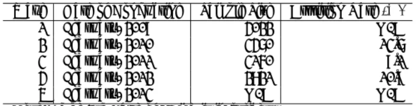
JHPS included a set of questionnaire to survey respondents’ preferable amount of tax and benefit for households in imaginary society. (Please see Appendix A.) The survey including this set of questionnaire was conducted in February, 2011 for the first time and also conducted in February, 2012. This section describes some features of this questionnaire.
JHPS started its first survey in 2009, and the JHPS survey in 2011 is the 3rd wave. The brief summary of the outcomes of JHPS survey since it started its survey in 2009 is described in Table 2.
Sampling design of JHPS is the two-stage stratified random sampling. Sur-vey areas of the Population Census of Japan are sampled in the 1st stage, and individuals are sampled in the 2nd stage. The JHPS questionnaire also includes a set of questions to ask spouse of the individual respondent to answer, if he or she has the one. The set of questions on preference for redistribution is only directed to respondents, but not to their spouses, in order to preserve random-ness in sampling. Exactly the same set of the questions listed in Appendix A in included in JHPS questionnaire in 2011 and 2012 as well, thus the outcome of this set of questions can be used as panel data of two periods.
Features of the set of questions to survey preference for redistribution in JHPS are as follows. First, it shows an imaginary society consisting of three
5Appendix A shows this set of questionnaire.
6Date of conducting JHPS in 2011 is February 2011. Soon after the JHPS started its
survey or while the survey was in process, the Great Earthquake of Eastern Japan occurred on March 11 in 2011.
households, and each of household consists of four members. The tree house-holds are named as “Household A,” “Household B” and “Household C.” It also shows initial income of each household as 35 thousand USD, 70 thousand USD and 125 thousand USD7 for Household A, Household B and Household C re-spectively. These initial income was obtained as the rounded mean of the lower 33%, middle 33% and higher 33% of the initial income distribution of re-sampled households which consist of four members in JHPS 2009 survey8.
The formula of calculating Gini coefficient is formula (2.8.3) in Sen and Foster(1973). The Gini coefficient of the initial income distribution in this imaginary society is 0.2609, and this value is much smaller than the actual Gini coefficient of Japan, 0.462, listed in Table 1. Limiting the households in the imaginary society to four-member household might have excluded the poor households from the sample and this might have caused the gap between the Gini coefficient in the imaginary society and that of real society.
Given this initial income distribution in the imaginary society, the question (1) in the JHPS questionnaire asks each respondent to answer
• the most preferable amounts of Tax and Social Security Contribution that
each household pays, and
• the most preferable amounts of Social Security Benefit that each household
receives.
The question (2) in the JHPS questionnaire asks the preferable amount of Social Benefit if the household income happens to be zero due to loosing job.
The way to ask the preferable amount of tax and that of social security contribution has the following advantages.
1. Obtaining the tolerable measure of income inequality numerically, such as Gini coefficient, and this measure is comparable among different societies and countries. This type of numerical measure being comparable among different societies cannot be obtained by the answering format of one di-mensional measure to questions such as how much each respondent thinks the income inequality of the society is large9. Plans for analyses using
the outcome of this JHPS questionnaire is discussed in Yamamoto and Fukahori(2011).
2. Asking the preferable levy of tax and benefit of social security enables us to measure the preference for tax and benefit separately, even if these preferences are not symmetrical10.
7In original set of questionnaire, unit of the initial income of each household is yen, and
the amount in US dollars are converted from yen with the rate of 1USD= 100yen.
8The reason why re-sampling of households were performed, not for JHPS 2011, but for
JHPS 2009 survey was to avoid sampling bias due to sample attrition.
9See the item “INCGAP” in GSS questionnaire in Appendix B, for example.
10The term “symmetrical” here means that the effects of observed certain characteristic of
each respondent over the measure of preference for tax and that for social security benefit are opposite in direction to each other and that both effects are statistically significant.
3. The preferable amounts of tax and that of benefit enables us to obtain the preference for the size of government expenditure. This information can-not be obtained with questions asking whether or can-not the each respondent thinks the government tax rate is too large or not11.
4. The preferred slopes of tax and benefit over the initial income distribution are obtained. The slopes shows whether the preferences for tax and social security benefit are progressive or not over a specific pre-tax income distri-bution. The degree how much each respondent thinks the tax and benefit should be progressive over a given set of income distribution cannot be obtained by the way of asking the preference for the statement such that the rich should pay more tax than the poor should12.
The next section shows these advantages concretely with the results of anal-yses on the outcomes of the JHPS questionnaire to measure the preference for redistribution.
4
Summary of the Outcomes of JHPS
Question-naire on Preference for Redistribution
The Great Earthquake of Eastern Japan of 2011 (abbreviated as “GEEJ” in this paper) occurred on March 11, 2011 between the JHPS surveys in 2011 and in 2012. This section summarizes the outcomes of JHPS questionnaire on preference for tax and benefit surveyed in 2011 and in 2012 with a setting of treatment group and control group where the respondents in cities suffered from severe aftermath of GEEJ form the treatment group.
Table 3 summarizes the outcome in the form of the table in the questionnaire of Question (1) presented in the Appendix A. In this table, the outcomes of respondents are divided into two groups, i.e. “Treatment Group” and ”Control Group.” The “Treatment Group” consists of the outcomes of the respondents who are in the areas that the “Disaster Relief Act” was applied for due to the GEEJ13, and the “Control Group” consists of the outcomes of the respondents
11See the item “TAXRICHI” in GSS questionnaire in Appendix B, for example.
12See the items “GOVEQINC” and “TAXSHARE” in GSS questionnaire in Appendix B,
the item “V152” in WVS questionnaire in Appendix D, the item “D23” in ESS questionnaire in Appendix C, for examples.
13As noted at the Note 1 in Table 3, although the Disaster Relief Act was applied for cities
in Tokyo as well as other cities suffered from sever aftermath of the earthquake, tsunami and radiation emitted from the Fukushima Dai-ichi Nuclear Power Plant, the “Treatment Group” excludes all the outcomes of the respondent in Tokyo, and they are included in the “Control Group.” The reason is the application for the Disaster Relief Act to cities in Tokyo was mainly to supply food, water and blankets to workers who had difficulty in returning their homes from their offices in central Tokyo area due to the traffic turmoil soon after the earthquake occurred. Thus, the application of the Disaster Relief Act to cities in Tokyo ended much sooner compared to other cities that suffered from sever aftermath of the GEEJ. See also the Ministry of Health, Labour and Welfare of Japan Home Page “On application of Disaster Relief Act for Earthquake in Pacific Ocean along the coastal area of Tohoku(Report 11)” in references.
Table 3: Summary Statistics of Outcomes of the Questionnaire; Treatment Group of the GEEG vs. Control Group(JHPS2011,2012)
Panel I: Question(1); Outcomes on Tax and Social Security Benefit in Imaginary Society Amount of Tax and Social Amount of Social
Security Contribution Security Benefit that Government should collect Government should expend
2011 2012 2011 2012 n 183 159 n 183 159 Treatment Group (134) (134) (134) (134) mean 21.64 22.98 mean 58.93 73.84 (24.22) (23.51) (64.16) (67.96) s.d. 26.79 23.02 s.d. 75.97 91.12 Household A (28.79) (23.58) (81.98) (85.04) (35 thousand USD) n 2374 2137 n 2374 2137 (1942) (1942) (1942) (1942) mean 23.12 21.66 mean 59.82 59.56 (23.48) (21.84) (58.76) (59.71) Control Group s.d. 25.78 22.82 s.d. 77.40 82.66 (26.34) (23.09) (76.10) (81.89) mean 68.93 68.60 mean 28.15 55.40 Treatment Group (74.08) (68.96) (35.28) (49.19) s.d. 61.41 54.76 s.d. 75.87 115.58 Household B (63.39) (54.66) (87.00) (106.70) (70 thousand USD) mean 72.16 69.31 mean 37.06 46.87
(72.97) (69.78) (36.31) (47.53) Control Group s.d. 58.63 56.84 s.d. 90.21 106.11 (57.02) (56.18) (88.08) (105.34) mean 168.62 173.25 mean 33.92 62.08 Treatment Group (176.07) (170.64) (42.57) (55.53) s.d. 147.07 137.23 s.d. 125.18 172.62 Household C (151.13) (134.92) (144.39) (159.48) (125 thousand USD) mean 176.74 169.29 mean 41.45 45.73
(179.23) (170.97) (40.34) (46.06) Control Group s.d. 139.54 135.40 s.d. 134.40 144.30 (137.74) (135.59) (132.89) (144.36) Panel II: Question(2); Outcomes on Social Security for Loosing Job
2011 2012
n 183 159
(134) (134)
Treatment Group mean 192.53 199.36 (193.97) (192.34) s.d. 119.32 115.00
(125.70) (107.81)
n 2374 2137
(1942) (1942)
Control Group mean 204.35 203.15 (205.72) (204.02) s.d. 108.71 109.51
(107.36) (109.08)
Note1) Outcomes of respondents in cities in Tokyo are classified into the Control Group.
Note2) Panel I: The sample size(n)’s for Household B and C are same as those for Household A in each corresponding cell.
Note3) Each value outside the parentheses represents the statistic of independent sample of 2011 as well as 2012. Note4) Each value inside the parentheses represents the statistic of panel sample of 2011 through 2012.
in other cities.
Panel I in Table 3 describes the sample size(n)’s, means and standard de-viation(s.d.)’s of the outcomes for Question (1), which are divided into the “Treatment Group” and the “Control Group.” The each value in the parenthe-sis represents the outcomes for panel sample of 2011 through 2012 that excludes the dropped records in the JHPS 2012 sample, and the each value outside the parenthesis represents the outcomes for each sample in JHPS 2011 and in JHPS 2012 independently.
The Panel I of Table 3 shows different trends between outcomes on tax and those on social security benefit.
The s.d.’s of the outcomes on taxation tend to get smaller toward 2012 both in Treatment Group and Control Group. This trend looks similar both in independent samples for 2011 and 2012, as well as panel sample of 2011 through 2012. On the other hand, the s.d.’s of the outcomes on social security benefit tend to get a little larger toward 2012.
As for the means of the outcomes on taxation, the trend toward 2012 looks different between these for independent samples and that for panel sample. In case of Treatment Group, the means tend to get larger toward 2012 as for in-dependent samples, while the means in the panel sample tend to get smaller toward 2012. This implies sample attrition in such a way in which more re-spondents who prefer small amount of taxation dropped in 2012 survey than the respondents who prefer larger amount of taxation did.
5
Difference in Differences: Measuring Effect of
the Great Earthquake of Eastern Japan on
Preference for Redistribution
This section presents the results of measuring effect of the GEEJ on preference for redistribution by exploiting the outcomes of the panel sample of JHPS 2011 and 2012, with the method of the Difference in Differences(DID).
The DID was applied by Ashenfelter and Card(1985) to estimate the effect of job training program on wage profile using longitudinal data. Card(1990), Card and Krueger(1994) also estimated the impact of policies on labor market with this method. The GEEJ is considered absolutely exogenous to preference, so that the problem of endogeneity discussed by Ashenfelter and Card(1985) never arises in this DID analysis14 on the effect of GEEJ over preference for
redistribution.
14The problem of sample bias due to the sample attrition between JHPS 2011 and 2012
Table 4: Difference in Differences: Treatment Group of Cities where Disaster Relief Act was Applied vs. Control Group
Panel I: Amount of Net Income Transfer (Social Security Benefit minus Tax) Diff. in Treatment Gr. Diff. in Control Gr.
n mean s.d. n mean s.d. F Pr.F t Pr.t W Hous. A 134 4.50 98.1 1942 2.58 98.4 1.01 0.496 0.22 0.827 0 Hous. B 134 19.04 126.0 1942 14.40 134.6 1.14 0.165 0.39 0.698 0 Hous. C 134 18.39 220.5 1942 13.97 216.5 1.04 0.371 0.23 0.820 0 Panel II: Outcomes on Tax and Social Security Benefit(SSB) of Question(1)
Diff. in Treatment Gr. Diff. in Control Gr.
n mean s.d. n mean s.d. F Pr.F t Pr.t W Tax Hous. A 134 −0.70 28.8 1942 −1.64 30.4 1.11 0.211 0.35 0.729 0 Tax Hous. B 134 −5.13 65.6 1942 −3.18 68.4 1.09 0.267 0.32 0.750 0 Tax Hous. C 134 −5.43 164.1 1942 −8.26 151.4 1.18 0.090 0.21 0.835 0 SSB Hous. A 134 3.80 99.6 1942 0.94 98.9 1.01 0.443 0.32 0.747 0 SSB Hous. B 134 13.92 120.1 1942 11.22 124.8 1.08 0.285 0.24 0.808 0 SSB Hous. C 134 12.96 187.8 1942 5.72 177.7 1.12 0.179 0.45 0.649 0 Panel III: Amount of Government Expenditure: Total Amount of Social Security Benefit minus That of Tax
Diff. in Treatment Gr. Diff. in Control Gr.
n mean s.d. n mean s.d. F Pr.F t Pr.t W 134 41.93 386.9 1942 30.96 384.9 1.01 0.453 0.32 0.750 0 Panel IV: Outcome on the Amount of Social Security Benefit for Loosing Job of Question(2)
Diff. in Treatment Gr. Diff. in Control Gr.
n mean s.d. n mean s.d. F Pr.F t Pr.t W 134 −1.63 131.5 1942 −1.70 123.9 1.13 0.163 0.01 0.995 0 Panel V: Slope of Regression Line of Tax and SSB on the Pre-Tax Income
Diff. in Treatment Gr. Diff. in Control Gr.
n mean s.d. n mean s.d. F Pr.F t Pr.t W Tax Slope 134 −0.00483 0.1726 1942 −0.00752 0.1600 1.16 0.103 0.19 0.852 0 SSB Slope 134 0.00912 0.1705 1942 0.00394 0.1640 1.08 0.256 0.35 0.724 0 Panel VI: Slope of Regression Line of Net Income Transfer on the Pre-Tax Income
Diff. in Treatment Gr. Diff. in Control Gr.
n mean s.d. n mean s.d. F Pr.F t Pr.t W Slope 134 0.01395 0.2333 1942 0.01146 0.2310 1.02 0.425 0.12 0.904 0 Panel VII: Gini Coefficient of Income Distribution Caused by Taxation Only
Diff. in Treatment Gr. Diff. in Control Gr.
n mean s.d. n mean s.d. F Pr.F t Pr.t W 134 0.00045 0.0307 1942 0.00063 0.0318 1.08 0.297 0.06 0.951 0 Panel VIII: Gini Coefficient of Income Distribution Caused by Redistribution by Way of Social Security Benefit Only
Diff. in Treatment Gr. Diff. in Control Gr.
n mean s.d. n mean s.d. F Pr.F t Pr.t W 134 −0.00029 0.0303 1942 −0.00032 0.0303 1.00 0.478 0.01 0.993 0 Panel IX: Gini Coefficient of Income Distribution Caused by Net Income Transfer (Social Security Benefit minus Tax)
Diff. in Treatment Gr. Diff. in Control Gr.
n mean s.d. n mean s.d. F Pr.F t Pr.t W 134 0.00088 0.0482 1942 0.00071 0.0495 1.05 0.353 0.04 0.969 0 Note1) The Welch-Test is applied if the null hypothesisH0is rejected for 5% significant level inF -Test.
Table 4 shows the results of the DID analysis. Each row of the table shows a test for a certain index in DID formula. The table shows the each difference between the transitory differences of 2011 through 2012 in treatment group for certain specific index and the transitory difference of 2011 through 2012 in control group for the same index in the treatment group. The differences of 2011 through 2012 are obtained by panel sample. “F” in the table shows values of the test statistic for testing the null hypothesis that states the variances of the two groups are equal, and “Pr.P” represents the corresponding P-values. “t” in the table shows values of the test statistic for testing the null hypothesis that states the mean of the two groups are equal, and “Pr.t” in the table represents the corresponding P-values. If the hypothesis is rejected in significant level of 5% in F-Test, the Welch-Test is applied instead of t-test. The “W” in the rightmost column in the table indicates each flag that shows whether or not the Welch-Test was applied to an index of each row. The value 1 of the flag means the Welch-Test was applied, and 0 means not.
Indexes subject to statistical test in DID formula were as follows. (Panel I) indicates the test results for the amount of net income transfer, which is defined as the amount of benefit minus the amount of tax in the outcomes of Question(1), for each household. (Panel II) indicates the test results for the each outcome of Question (1), which decomposes the amount of net income transfer, listed in Panel I, into tax and social security benefit. (Panel III) indicates the test result for the amount of government expenditure, which is defined as total amount of benefit minus total amount of tax. (Panel IV) indicates the test result for the outcome of Question (2), where the respondent answers the preferable amount of social security benefit in case the household’s income happens to fall to zero due to loosing job. (Panel V) indicates the test results for the slope of regression line, which is obtained by fitting the line regressing the amount of tax or that of social security benefit of each household on the initial income15.
(Panel VI) also indicates the test result for the slope of regression line, which is obtained by fitting the line regressing the amount of net income transfer (social security benefit minus tax) for each household on the initial income. This slope aggregates the slopes for the Panel V and indicates whether or not the net transfer is progressive to initial income. (Panel VII) indicates the test result for Gini coefficient obtained by the income distribution caused by taxation only for each household. (Panel VIII) indicates the test result for Gini coefficient obtained by the income distribution caused by redistribution by way of social security benefit only for each household. Finally, (Panel IX) indicates the test result for Gini coefficient obtained by the income distribution caused by net transfer for each household.
Table 4 shows no evidence of significant shift in preference for redistribution in Treatment Group compared to that in Control Group. But this result does not deny the possibility that the GEEJ shifted preference for redistribution of Japanese constituency as a whole.
15In this paper, the phrase “initial income” is solely defined and used for the income
distri-bution before any kind of income transfer is applied in the imaginary society given in JHPS questionnaire on preference for redistribution.
6
Checking the Stability in Preference for
Re-distribution: Comparison of Cross-Section
Anal-ysis for JHPS 2011 and 2012
In the previous section, no significant shift in preference for redistribution be-tween the two groups was detected. This section discuss the stability in the relationship between each index obtained by outcomes of JHPS questionnaire on preference for redistribution and the observed characteristics of the each re-spondent over the two periods of JHPS survey year, i.e. the year of 2011 and 2012. In other words, this section presents the result of cross-section analysis performed independently for JHPS 2011 outcomes and JHPS 2012 outcomes to see what kind of observed characteristic systematically shifts the preference for redistribution.
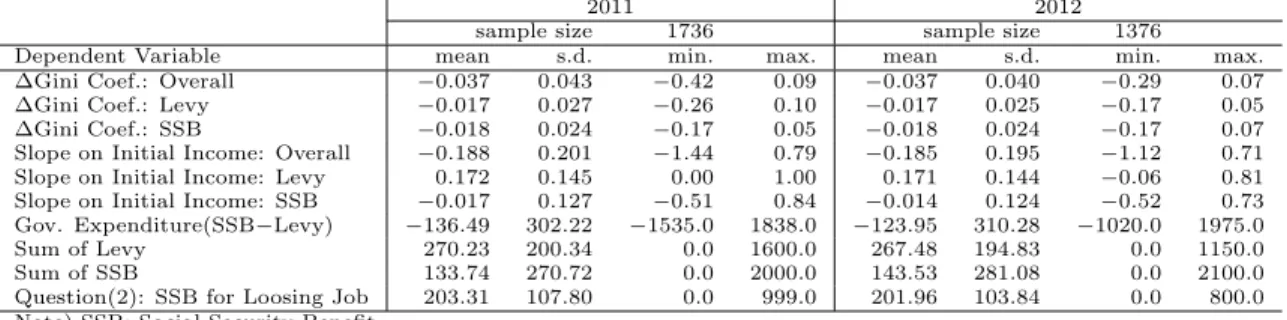
Panel I of the Table 5 shows the summary statistics of the dependent vari-ables. These dependent variables are classified into four groups.
First group is the differences in the value of Gini coefficient, which are cal-culated for the income distribution after income transfer is performed by means of tax, social security benefit or both of them that each respondent prefers, from the initial value of Gini coefficient, 0.2609, which is also calculated for the initial income distribution given in the imaginary society of the questionnaire of JHPS16. The difference in Gini coefficient is calculated based on the outcomes
of JHPS questionnaire, and three kinds of differences in Gini coefficient are de-fined. First, the difference caused by net income transfer by means of both tax and social security benefit. This difference is decomposed into the following two kinds of differences. The one is the difference caused by altering the income distribution solely by means of tax, and the other is the difference caused by altering the income distribution solely by means of social security benefit.
The second group is the slopes of the regression line, which is obtained by fitting the line regressing the amount of tax, that of social security benefit, or the amount of net income transfer of each household on the initial income. Three kinds of the slopes are defined, according to what amount to be regressed on the initial income. The first slope is obtained by regressing the amount of net income transfer for each household on the initial income. This slope is decomposed into the following two kinds of slopes. The one is the slope obtained by regressing the amount of tax on the initial income, and the other is obtained by regressing the amount of social security benefit on the initial income.
The third group is the sums of the amount of tax, social security benefit and net income transfer across three households in the imaginary society. This sum indicates the scale of the government budget or deficit due to redistribution policy of the government. Three kinds of sums are defined, according to what amount to be summed up. The first is the sum of the each amount of the net 16Because the value of Gini coefficient is zero under the circumstance of perfectly equal
income distribution, the difference in the value of Gini coefficient will be negative if the income redistribution policy gets the distribution closer, in terms of Gini coefficient, to the perfectly equalized income distribution than the initial income distribution is.
income transfer for each household. This sum is decomposed into the following two kinds of sums. The one is the sum of the each amount of tax that each household pay, and the other is the sum of the each amount of social security benefit that each household receives.
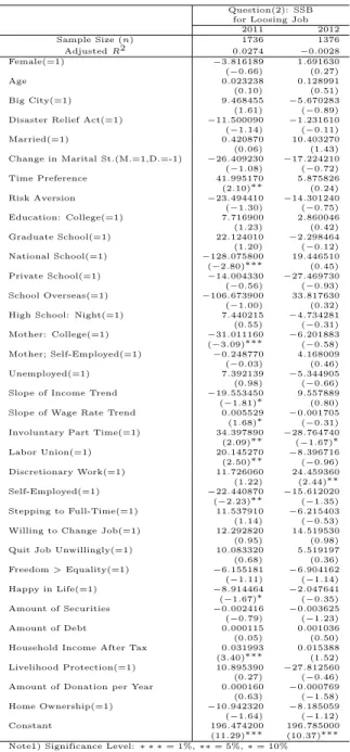
The fourth group, although consisting of only one element, is the outcome of Question (2) which asks the respondents how much amount of the social security benefit should be in case the household income falls to zero due to loosing job. Independent variables are shown in Panel II in Table 5. Those independent variables are classified into some groups in terms of the observed characteristics of respondents. First, “Female” or gender, and “Age” represent demographical status. Second, “Big City” and “Disaster Relief Act” represent geographical status. Third, “Married” and “Change in Marital St.” represent marital status. The variable “Change in Marital St.” represents change in marital status in the survey year compared to that in one year before, and takes the value of zero, 1, −1 for the case of unchanged, married and divorced respectively. Fourth, “Time Preference” and “Risk Aversion” represent behavioral preference of each respondent. The variable of “Time Preference” represents discounting and is cal-culated as the interest rate for the outcomes to the question how much amount of money satisfies you if you have to wait for 13 months instead of receiving 100 dollars one month from now. The variable of “Risk Aversion” takes the value of minimum probability at which the respondent brings an umbrella when he or she goes out for a place that he or she has never visited before. This variable takes the value of zero, if the respondent answers that he or she always takes an um-brella unconditionally. Fifth, “Education: College,” “Graduate School,” “Na-tional School,” “Private School,” “School Overseas” and “High School: Night” represent the educational background of each respondent. “National School,” “Private School” and “School Overseas” are dummy variables. Each takes a value of one when the respondent went elementary school or high school of that category, and zero otherwise. These three variables might reflect the parents’ (of each respondent) attitude toward society. “High School: Night” takes value of one when respondent went night course of high school, and zero otherwise. This variable also might reflect the situation of the respondent’s family background because tuition fee of the night course is very cheap, and many students go to night course while they work in daytime. This may imply that the family of the respondent when he or she was about age of 15 years was relatively poor. Sixth, “Mother: College” and “Mother: Self-Employed” represent the parents’ (of the respondent) background and may represent the parents’ attitude toward society. Seventh, “Unemployment,” “Slope of Income Trend,” “Slope of Wage Rate Trend,” “Involuntary Part Time,” “Labor Union,” “Discretionary Work,” “Self-Employed,” “Stepping t Full-Time,” “Willing to Change Job” and “Quit Job Unwillingly” represent employment status of each respondent. “Involuntary Part Time” takes a value of one when the respondent only has part time job opportunity although he or she wants to have full time job opportunity, and zero otherwise. “Stepping to Full-Time” takes a value of one when the respondent is currently in a position of time job but the chance to step up to the posi-tion of full time job is open to the respondent at the establishment where the
respondent currently works, and zero otherwise. Eighth, “Freedom > Equal-ity” represents the political attitude of each respondent, which takes a value of one he or she believes freedom is more important than equality in this society. Ninth, “Happy in Life” represents mental situation of each respondent, which takes a value of one when the respondent thinks he or she is happy in whole life. Tenth, “Amount of Securities,” “Amount of Debt,” “Household Income After Tax,” “Livelihood Protection” and “Home Ownership” represent economic sit-uation of each respondent’s household. “Livelihood Protection” takes a value of one if livelihood protection service by government is granted to the household of each respondent because the household suffers form an extreme poverty. “Home Ownership” takes a value of one when the family of each respondent owns the dwelling. Finally, “Amount of Donation per Year” represents each respondent’s attitude toward society. These variables are chosen according to hypotheses in the literature.
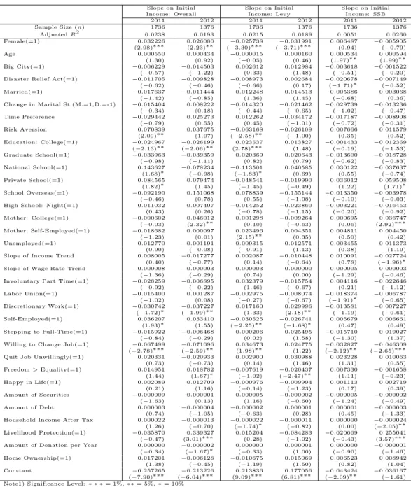
Table 6 through Table 9 show the results of cross-section analysis for JHPS 2011 and 2012 separately and independently. Table 6 shows the results of re-gression analysis where the dependent variables of the group 1 are regressed on observed characteristics of the respondent. Table 7 shows the results of re-gression analysis where the dependent variables of the group 2 are regressed on observed characteristics of the respondent. Table 8 shows the results of re-gression analysis where the dependent variables of the group 3 are regressed on observed characteristics of the respondent. Table 9 shows the results of re-gression analysis where the dependent variable of the group 4 is regressed on observed characteristics of the respondent.
Table 5: Summary Statistics of Dependent Variables and Independent Variables
Panel I: Summary Statistics of Dependent Variables
2011 2012
sample size 1736 sample size 1376
Dependent Variable mean s.d. min. max. mean s.d. min. max. ΔGini Coef.: Overall −0.037 0.043 −0.42 0.09 −0.037 0.040 −0.29 0.07 ΔGini Coef.: Levy −0.017 0.027 −0.26 0.10 −0.017 0.025 −0.17 0.05 ΔGini Coef.: SSB −0.018 0.024 −0.17 0.05 −0.018 0.024 −0.17 0.07 Slope on Initial Income: Overall −0.188 0.201 −1.44 0.79 −0.185 0.195 −1.12 0.71 Slope on Initial Income: Levy 0.172 0.145 0.00 1.00 0.171 0.144 −0.06 0.81 Slope on Initial Income: SSB −0.017 0.127 −0.51 0.84 −0.014 0.124 −0.52 0.73 Gov. Expenditure(SSB−Levy) −136.49 302.22 −1535.0 1838.0 −123.95 310.28 −1020.0 1975.0 Sum of Levy 270.23 200.34 0.0 1600.0 267.48 194.83 0.0 1150.0 Sum of SSB 133.74 270.72 0.0 2000.0 143.53 281.08 0.0 2100.0 Question(2): SSB for Loosing Job 203.31 107.80 0.0 999.0 201.96 103.84 0.0 800.0 Note) SSB: Social Security Benefit
Panel II: Summary Statistics of Independent Variables
2011 2012
sample size 1736 sample size 1376
Independent Variable mean s.d. min. max. mean s.d. min. max.
Female(=1) 0.460 0.499 0 1 0.467 0.499 0 1
Age 50.50 15.09 22.0 90.0 50.50 14.81 23.0 91.0
Big City(=1) 0.278 0.448 0 1 0.289 0.454 0 1
Disaster Relief Act(=1) 0.070 0.256 0.00 1.00 0.065 0.246 0.00 1.00
Married(=1) 0.771 0.420 0 1 0.767 0.423 0 1 Change in Marital St.(M.=1,D.=-1) 0.001 0.107 −1.00 1.00 0.000 0.121 −1.00 1.00 Time Preference 0.225 0.131 −0.05 0.95 0.210 0.116 −0.03 0.78 Risk Aversion 0.423 0.148 0.00 1.00 0.413 0.155 0.00 1.00 Education: College(=1) 0.290 0.454 0 1 0.298 0.458 0 1 Graduate School(=1) 0.022 0.146 0 1 0.025 0.155 0 1 National School(=1) 0.003 0.059 0 1 0.004 0.066 0 1 Private School(=1) 0.011 0.104 0 1 0.009 0.097 0 1 School Overseas(=1) 0.001 0.024 0 1 0.001 0.027 0 1 High School: Night(=1) 0.039 0.193 0 1 0.038 0.191 0 1 Mother: College(=1) 0.079 0.271 0 1 0.085 0.279 0 1 Mother; Self-Employed(=1) 0.119 0.324 0 1 0.118 0.322 0 1 Unemployed(=1) 0.270 0.444 0 1 0.270 0.444 0 1 Slope of Income Trend 0.07 0.25 −2.3 3.0 0.07 0.25 −1.1 2.9 Slope of Wage Rate Trend 24.18 787.45 −6636.5 6870.0 24.72 514.58 −3475.2 3329.4 Involuntary Part Time(=1) 0.027 0.162 0 1 0.030 0.170 0 1 Labor Union(=1) 0.136 0.343 0 1 0.136 0.343 0 1 Discretionary Work(=1) 0.093 0.291 0 1 0.105 0.307 0 1 Self-Employed(=1) 0.090 0.286 0 1 0.079 0.270 0 1 Stepping to Full-Time(=1) 0.078 0.269 0 1 0.068 0.252 0 1 Willing to Change Job(=1) 0.043 0.203 0 1 0.041 0.198 0 1 Quit Job Unwillingly(=1) 0.032 0.175 0 1 0.036 0.187 0 1 Freedom> Equality(=1) 0.334 0.472 0 1 0.337 0.473 0 1 Happy in Life(=1) 0.547 0.498 0 1 0.525 0.500 0 1 Amount of Securities 227.18 866.72 0.0 24000.0 235.25 998.04 0.0 24000.0 Amount of Debt 604.71 1283.64 0.0 20000.0 672.95 1458.54 0.0 18000.0 Household Income After Tax 506.34 295.99 0.0 3500.0 509.94 304.59 0.0 3000.0 Livelihood Protection(=1) 0.004 0.063 0 1 0.002 0.047 0 1 Amount of Donation per Year 1604.0 10731.2 0. 320000. 1256.3 5874.7 0. 100000. Home Ownership(=1) 0.770 0.421 0 1 0.767 0.423 0 1 Note) “(=1)” after the variable name indicates that the variable is a dummy variable.
Table 6: Δ Gini Coefficients
ΔGini Coef. ΔGini Coef. ΔGini Coef.
Overall Levy SSB 2011 2012 2011 2012 2011 2012 Sample Size (n) 1736 1376 1736 1376 1736 1376 AdjustedR2 0.0236 0.0223 0.0157 0.0175 0.0154 0.0273 Female(=1) 0.006775 0.003831 0.003625 0.004751 0.002769 −0.000634 (2.93)∗∗∗ (1.58) (2.51)∗∗ (3.19)∗∗∗ (2.18)∗∗ (−0.45) Age −0.000086 −0.000132 −0.000086 −0.000101 −0.000016 −0.000063 (−0.95) (−1.36) (−1.51) (−1.68)∗ (−0.32) (−1.12) Big City(=1) −0.000798 −0.002975 −0.000101 −0.002365 −0.000834 −0.000817 (−0.34) (−1.21) (−0.07) (−1.56) (−0.65) (−0.57)
Disaster Relief Act(=1) −0.001564 −0.005011 0.000977 0.000756 −0.002553 −0.005916
(−0.39) (−1.12) (0.39) (0.28) (−1.15) (−2.27)∗∗ Married(=1) −0.002866 −0.001675 −0.001850 −0.001826 −0.000401 0.000167 (−1.08) (−0.60) (−1.11) (−1.06) (−0.27) (0.10) Change in Marital St.(M.=1,D.=-1) 0.006866 0.000603 0.001657 0.002882 0.004718 −0.002229 (0.70) (0.07) (0.27) (0.51) (0.88) (−0.41) Time Preference −0.014782 0.001378 −0.008506 −0.000965 −0.005985 0.001941 (−1.85)∗ (0.15) (−1.70)∗ (−0.17) (−1.36) (0.35) Risk Aversion 0.013095 0.011412 0.011014 0.001669 0.001896 0.008888 (1.80)∗ (1.56) (2.42)∗∗ (0.37) (0.48) (2.08)∗∗ Education: College(=1) −0.005587 −0.004605 −0.002388 −0.000786 −0.002989 −0.002895 (−2.23)∗∗ (−1.76)∗ (−1.52) (−0.49) (−2.17)∗∗ (−1.89)∗ Graduate School(=1) 0.000079 −0.002585 −0.002640 0.003053 0.002465 −0.003269 (0.01) (−0.35) (−0.57) (0.68) (0.61) (−0.76) National School(=1) 0.034695 −0.038151 0.013736 −0.005256 0.018970 −0.028337 (1.89)∗ (−2.32)∗∗ (1.20) (−0.52) (1.88)∗ (−2.95)∗∗∗ Private School(=1) 0.013232 0.018312 0.007088 0.004074 0.003805 0.012207 (1.33) (1.61) (1.14) (0.58) (0.70) (1.84)∗ School Overseas(=1) −0.010989 0.031711 −0.021209 0.019241 0.009517 0.011349 (−0.26) (0.79) (−0.79) (0.78) (0.40) (0.48)
High School: Night(=1) 0.004685 0.002237 0.003449 0.005952 0.001233 −0.002998
(0.86) (0.38) (1.01) (1.66)∗ (0.41) (−0.88) Mother: College(=1) −0.003001 0.006902 −0.002893 −0.000482 −0.000075 0.006084 (−0.75) (1.68)∗ (−1.15) (−0.19) (−0.03) (2.54)∗∗ Mother; Self-Employed(=1) −0.003716 −0.001545 −0.004611 −0.001356 0.000631 −0.000106 (−1.15) (−0.45) (−2.27)∗∗ (−0.64) (0.35) (−0.05) Unemployed(=1) 0.002981 0.001823 0.002959 −0.001267 −0.000300 0.002930 (0.99) (0.58) (1.56) (−0.66) (−0.18) (1.61)
Slope of Income Trend 0.000986 −0.008138 −0.001042 −0.000184 0.001319 −0.006412
(0.23) (−1.77)∗ (−0.38) (−0.06) (0.55) (−2.38)∗∗
Slope of Wage Rate Trend −0.000002 0.000000 −0.000001 0.000000 −0.000001 0.000000
(−1.71)∗ (0.14) (−0.75) (0.34) (−2.01)∗∗ (−0.14)
Involuntary Part Time(=1) −0.006428 −0.001070 −0.006149 0.001820 −0.000509 −0.002190
(−0.98) (−0.16) (−1.49) (0.45) (−0.14) (−0.57) Labor Union(=1) −0.004120 −0.000451 0.000472 0.001796 −0.004262 −0.002264 (−1.28) (−0.13) (0.23) (0.86) (−2.40)∗∗ (−1.15) Discretionary Work(=1) −0.005855 −0.008936 −0.001580 −0.006465 −0.003749 −0.002117 (−1.53) (−2.32)∗∗ (−0.66) (−2.72)∗∗∗ (−1.78)∗ (−0.94) Self-Employed(=1) 0.010835 0.006683 0.005211 0.004626 0.005059 0.001661 (2.69)∗∗∗ (1.50) (2.07)∗∗ (1.69)∗ (2.29)∗∗ (0.64) Stepping to Full-Time(=1) −0.001530 −0.004363 −0.000506 −0.005136 −0.000609 0.000461 (−0.38) (−0.96) (−0.20) (−1.84)∗ (−0.27) (0.17)
Willing to Change Job(=1) −0.012591 −0.017363 −0.004344 −0.003747 −0.006315 −0.011983
(−2.43)∗∗ (−3.06)∗∗∗ (−1.34) (−1.07) (−2.21)∗∗ (−3.61)∗∗∗
Quit Job Unwillingly(=1) −0.000203 −0.006723 0.002570 −0.006717 −0.001957 −0.001110
(−0.03) (−1.13) (0.69) (−1.83)∗ (−0.60) (−0.32) Freedom> Equality(=1) 0.004243 0.007037 0.001965 0.004161 0.002292 0.002764 (1.92)∗ (3.03)∗∗∗ (1.42) (2.91)∗∗∗ (1.88)∗ (2.04)∗∗ Happy in Life(=1) 0.000794 0.000567 −0.000003 0.001007 0.000600 −0.000700 (0.37) (0.25) (0.00) (0.72) (0.51) (−0.53) Amount of Securities −0.000001 0.000001 −0.000001 0.000000 0.000000 0.000001 (−0.87) (1.02) (−0.70) (0.61) (−0.56) (1.13) Amount of Debt 0.000000 −0.000001 0.000000 0.000000 0.000000 0.000000 (0.48) (−0.84) (0.29) (−0.76) (0.36) (−0.54)
Household Income After Tax 0.000003 −0.000001 0.000005 0.000002 −0.000002 −0.000003
(0.79) (−0.33) (2.11)∗∗ (1.02) (−0.88) (−1.31)
Livelihood Protection(=1) −0.001012 0.023542 −0.003670 0.008220 0.002987 0.012590
(−0.06) (1.01) (−0.36) (0.57) (0.33) (0.93)
Amount of Donation per Year 0.000000 0.000000 0.000000 0.000000 0.000000 0.000000
(−0.65) (−1.92)∗ (−0.13) (−0.69) (−0.88) (−2.00)∗∗
Home Ownership(=1) 0.007093 −0.002635 0.003411 −0.002398 0.003307 −0.000692
(2.66)∗∗∗ (−0.94) (2.04)∗∗ (−1.39) (2.26)∗∗ (−0.42)
Constant −0.042447 −0.031445 −0.021134 −0.012780 −0.018855 −0.015543
(−6.09)∗∗∗ (−4.31)∗∗∗ (−4.84)∗∗∗ (−2.85)∗∗∗ (−4.92)∗∗∗ (−3.65)∗∗∗
Note1) Significance Level:∗ ∗ ∗ = 1%, ∗∗ = 5%, ∗ = 10%
Note2) Values in parentheses aret-values.