Research Article
Tomographic Image Reconstruction Based on Minimization of
Symmetrized Kullback-Leibler Divergence
Ryosuke Kasai
,
1Yusaku Yamaguchi
,
2Takeshi Kojima
,
3and Tetsuya Yoshinaga
31Graduate School of Health Sciences, Tokushima University, 3-18-15 Kuramoto, Tokushima 770-8509, Japan 2Shikoku Medical Center for Children and Adults, 2-1-1 Senyu, Zentsuji 765-8507, Japan
3Institute of Biomedical Sciences, Tokushima University, 3-18-15 Kuramoto, Tokushima 770-8509, Japan
Correspondence should be addressed to Tetsuya Yoshinaga; [email protected] Received 3 April 2018; Revised 8 June 2018; Accepted 26 June 2018; Published 17 July 2018 Academic Editor: Elena Zaitseva
Copyright © 2018 Ryosuke Kasai et al. This is an open access article distributed under the Creative Commons Attribution License, which permits unrestricted use, distribution, and reproduction in any medium, provided the original work is properly cited. Iterative reconstruction (IR) algorithms based on the principle of optimization are known for producing better reconstructed images in computed tomography. In this paper, we present an IR algorithm based on minimizing a symmetrized Kullback-Leibler divergence (SKLD) that is called Jeffreys’ 𝐽-divergence. The SKLD with iterative steps is guaranteed to decrease in convergence monotonically using a continuous dynamical method for consistent inverse problems. Specifically, we construct an autonomous differential equation for which the proposed iterative formula gives a first-order numerical discretization and demonstrate the stability of a desired solution using Lyapunov’s theorem. We describe a hybrid Euler method combined with additive and multiplicative calculus for constructing an effective and robust discretization method, thereby enabling us to obtain an approximate solution to the differential equation. We performed experiments and found that the IR algorithm derived from the hybrid discretization achieved high performance.
1. Introduction
Various kinds of iterative reconstruction (IR) [1–4] algo-rithms based on the principle of optimization are known for producing better reconstructed images in computed tomog-raphy (CT). In accordance with the base objective function, each IR method has intrinsic properties in the quality of images and in the convergence of iterative solutions. The maximum-likelihood expectation-maximization (ML-EM) [4] algorithm decreases the generalized Kullback-Leibler (KL) divergence [5, 6] between the measured projection and the forward projection along with the iteration. However, the objective function, in which the multiplicative algebraic reconstruction technique (MART) [7–10] forces a decrease in the iterative process, is an alternative KL-divergence done by exchanging the measured and forward projections. Due to the asymmetry of the KL-divergence, both objective functions have generally different values.
In this paper, we present an IR algorithm based on the minimization of a symmetrized KL-divergence (SKLD),
which is formulated using the mean of the two mutually
alternative KL-divergences and is called Jeffreys’𝐽-divergence
[11, 12]. Because the base optimization function is a symmet-ric premetsymmet-ric measure and it gives an upper bound of the Jensen-Shannon divergence [13, 14], one can expect a better performance while preserving good properties of ML-EM and MART algorithms. The convergence to an exact solution and the monotonic decreasing of the SKLD with each iterative step for a consistent inverse problem are guaranteed using the approach of the continuous dynamical method [15– 20]. Specifically, we construct an autonomous differential equation for which the proposed iterative formula gives a first-order numerical discretization with some step size and demonstrate the stability of an equilibrium in a continuous-time system using Lyapunov’s stability theorem [21]. The theory is extended to a case where the Lyapunov function can
be an𝛼-skew 𝐽-divergence with a parameter 𝛼 ∈ [0, 1], which
is the SKLD when𝛼 = 0.5.
We also propose a novel method for constructing an effective and robust method in the discretization, thereby Volume 2018, Article ID 8973131, 9 pages
enabling us to obtain an approximate solution to the differ-ential equation. That is, a hybrid Euler discretization com-bined with additive and multiplicative calculus works well; however, neither additive nor multiplicative Euler method does.
We conducted experiments and found that the IR algo-rithm derived from the hybrid Euler discretization of the continuous-time dynamical system achieved high perfor-mance.
2. ML-EM and MART Algorithms
The problem of image reconstruction from measured
projec-tions in CT is formulated as solving unknown variable𝑥 ∈ 𝑅𝐽+
for pixel values such that
𝑦 = 𝐴𝑥 + 𝜎, (1)
where𝑦 ∈ 𝑅𝐼++,𝐴 ∈ 𝑅𝐼×𝐽+ , and𝜎 ∈ 𝑅𝐼represent the measured
projection, projection operator, and noise, respectively, with
𝑅+and𝑅++, respectively, denoting the sets of nonnegative and
positive real numbers. If the system𝑦 = 𝐴𝑥 has a nonnegative
solution, it is consistent; otherwise, it is inconsistent. We introduce the following definitions and notations. The
variable denoted by the symbol𝜆𝑗for𝑗 = 1, 2, . . . , 𝐽 is defined
by 𝜆𝑗fl (∑𝐼 𝑖=1 𝐴𝑖𝑗) −1 , (2)
where𝐴𝑖𝑗is the element in the𝑖th row and 𝑗th column of
𝐴. The notations 𝑧𝑗and𝐴𝑖indicate the𝑗th element and the
𝑖th row vector of the vector 𝑧 and the matrix 𝐴, respectively. The function KL(𝑝, 𝑞) of two nonnegative vectors 𝑝 and 𝑞 represents the generalized KL-divergence [5]:
KL(𝑝, 𝑞) = 𝐼 ∑ 𝑖=1 𝑝𝑖log𝑝𝑖 𝑞𝑖 + 𝑞𝑖− 𝑝𝑖. (3)
Known methods of reconstructing tomographic images in clinical CT are filtered back projection (FBP) as a transform method and IR as an optimization process. KL-divergence is a common measure for deriving IR algorithms, and it plays an important role in accordance with the axiom that minimizing the KL-divergence is equivalent to maximizing the likelihood function that is considered suit-able for reconstruction modeled with a probability
distribu-tion. The sequences{KL(𝑦, 𝐴𝑧(𝑛))}∞𝑛=0and{KL(𝐴𝑧(𝑛), 𝑦)}∞𝑛=0
decrease for the respective iterative sequences{𝑧(𝑛)}∞𝑛=0of the
ML-EM and the (simultaneous) MART algorithms defined by 𝑧𝑗(𝑛 + 1) = 𝑧𝑗(𝑛) 𝜆𝑗∑𝐼 𝑖=1 𝐴𝑖𝑗𝐴𝑦𝑖 𝑖𝑧 (𝑛) (4) and 𝑧𝑗(𝑛 + 1) = 𝑧𝑗(𝑛) exp (𝜆𝑗 𝐼 ∑ 𝑖=1𝐴𝑖𝑗 log 𝑦𝑖 𝐴𝑖𝑧 (𝑛)) (5) for𝑗 = 1, 2, . . . , 𝐽 with 𝑧(0) = 𝑥0∈ 𝑅𝐽++.
3. Proposed System
The IR algorithm proposed in this paper can be described using the following difference equation.
𝑧𝑗(𝑛 + 1) = 𝑧𝑗(𝑛) (1 + 𝛿𝑓𝑗(𝑧 (𝑛))) exp (𝛿𝑔𝑗(𝑧 (𝑛))) , (6)
where𝛿 > 0 is a parameter and where the functions 𝑓𝑗 and
𝑔𝑗are, respectively, defined by
𝑓𝑗(𝑧 (𝑛)) = (1 − 𝛼) 𝜆𝑗 𝐼 ∑ 𝑖=1𝐴𝑖𝑗( 𝑦𝑖 𝐴𝑖𝑧 (𝑛)− 1) (7) and 𝑔𝑗(𝑧 (𝑛)) = 𝛼𝜆𝑗∑𝐼 𝑖=1 𝐴𝑖𝑗log 𝑦𝑖 𝐴𝑖𝑧 (𝑛) (8)
for𝑗 = 1, 2, . . . , 𝐽, with 𝛼 ∈ [0, 1] and 𝑧(0) = 𝑥0∈ 𝑅𝐽++.
For investigating the dynamics of the difference system in (6), we give its continuous analog described using the differential equation: 𝑑𝑥𝑗(𝑡) 𝑑𝑡 = 𝜆𝑗𝑥𝑗(𝑡) 𝐼 ∑ 𝑖=1 𝐴𝑖𝑗 ⋅ ((1 − 𝛼) ( 𝑦𝑖 𝐴𝑖𝑥 (𝑡) − 1) + 𝛼 log 𝑦𝑖 𝐴𝑖𝑥 (𝑡)) (9)
for𝑗 = 1, 2, . . . , 𝐽 and 𝑡 ≥ 0 with 𝑥(0) = 𝑥0 ∈ 𝑅𝐽++. The term
“continuous analog” means that a numerical discretization of the differential equation is the same as the difference equation. The idea is based on the approach for solving a constrained tomographic inverse problem using nonlinear dynamical methods [22–25].
3.1. Theoretical Analysis. The theoretical results on the
continuous-time system in (9) are given. First, we show that a solution is possible to ensure positive values remain.
Proposition 1. If we choose an initial value 𝑥0 ∈ 𝑅𝐽
++for the
system in (9), the solution𝜙(𝑡, 𝑥0) remains in the subspace 𝑅𝐽++ for all𝑡 ≥ 0.
Proof. The vector field of the 𝑗th element of the system is
multiplied by𝑥𝑗; therefore, the derivative𝑑𝜙𝑗/𝑑𝑡 ≡ 0 holds
for any𝑗 on the subspace 𝑥𝑗 ≡ 0, which means the subspace
is invariant and which means any flow cannot pass through invariant subspace on the basis of the uniqueness property of solutions to the initial value problem. Hence, the trajectory
emanating from the initial value in𝑅++behaves in the
sub-state space. Let us define 𝐽𝛼(𝑥) fl (1 − 𝛼) KL (𝑦, 𝐴𝑥) + 𝛼KL (𝐴𝑥, 𝑦) =∑𝐼 𝑖=1(1 − 𝛼) (𝑦𝑖 log 𝑦𝑖 𝐴𝑖𝑥 + 𝐴𝑖𝑥 − 𝑦𝑖) + 𝛼 (𝐴𝑖𝑥 log𝐴𝑖𝑥 𝑦𝑖 + 𝑦𝑖− 𝐴𝑖𝑥) (10)
with𝛼 in the interval [0, 1] as an 𝛼-skew 𝐽-divergence. The function is essential for a premetric measure of difference
between𝑦 and 𝐴𝑥 in accordance with 𝐽𝛼(𝑥) ≥0 and 𝐽𝛼(𝑥) = 0
if and only if𝑦 = 𝐴𝑥. When 𝛼 = 0.5, the divergence 𝐽𝛼
becomes a symmetrical form of KL-divergence by averaging KL(𝑦, 𝐴𝑥) and KL(𝐴𝑥, 𝑦), which we abbreviate as SKLD.
Then, under the assumption that the inverse problem is consistent, the following shows that the solution converges to
a desired equilibrium and that the nonnegative function𝐽𝛼
monotonically decreases along solution trajectories.
Theorem 2. If a unique solution 𝑒 ∈ 𝑅𝐽
++exists to the system
𝑦 = 𝐴𝑥, the equilibrium 𝑒 of the dynamical system in (9) with
any𝛼 ∈ [0, 1] is asymptotically stable.
Proof. A Lyapunov candidate function, 𝐽𝛼, is defined for applying Lyapunov’s stability theorem in (10):
𝐽𝛼(𝑥) =∑𝐼 𝑖=1 (1 − 𝛼) ∫𝐴𝑖𝑥 𝑦𝑖 1 − 𝑦𝑤𝑖𝑑𝑤 + 𝛼 ∫𝐴𝑖𝑥 𝑦𝑖 log𝑤 𝑦𝑖 =∑𝐼 𝑖=1 (1 − 𝛼) [𝑤 − 𝑦𝑖log𝑤]𝐴𝑖𝑥 𝑦𝑖 + 𝛼 [𝑤 log𝑦𝑤 𝑖 − 𝑤] 𝐴𝑖𝑥 𝑦𝑖 , (11)
which is well defined via Proposition 1 when choosing an
initial value𝑥0 in𝑅𝐽++. We then calculate its derivative with
respect to the dynamical system in (9) with any𝛼 ∈ [0, 1] as
𝑑𝐽𝛼 𝑑𝑡 (𝑥)(9)= 𝐼 ∑ 𝑖=1((1 − 𝛼) (1 − 𝑦𝑖 𝐴𝑖𝑥) + 𝛼 log 𝐴𝑖𝑥 𝑦𝑖 ) ⋅∑𝐽 𝑗=1 𝐴𝑖𝑗𝑑𝑥𝑗 𝑑𝑡 = − 𝐽 ∑ 𝑗=1 𝐼 ∑ 𝑖=1 𝐴𝑖𝑗((1 − 𝛼) ( 𝑦𝑖 𝐴𝑖𝑥− 1) + 𝛼 ⋅ log 𝑦𝑖 𝐴𝑖𝑥) 𝜆𝑗𝑥𝑗 𝐼 ∑ 𝑘=1 𝐴𝑘𝑗((1 − 𝛼) ( 𝑦𝑘 𝐴𝑘𝑥 − 1) + 𝛼 ⋅ log 𝑦𝑘 𝐴𝑘𝑥) = − 𝐽 ∑ 𝑗=1(√𝜆𝑗 𝑥𝑗∑𝐼 𝑖=1 𝐴𝑖𝑗 ⋅ ((1 − 𝛼) ( 𝑦𝑖 𝐴𝑖𝑥 − 1) + 𝛼 log 𝑦𝑖 𝐴𝑖𝑥)) 2 ≤ 0. (12)
The derivative equals zero at𝑥 = 𝑒 ∈ 𝑅𝐽++. Consequently, the
system has a Lyapunov function, so the equilibrium𝑒 of the
system is asymptotically stable.
3.2. Hybrid Euler Discretization. Consider an autonomous
differential equation for the state variable𝑥(𝑡) > 0, 𝑡 ≥ 0,
written by 𝑑𝑥 (𝑡)
𝑑𝑡 = 𝑥 (𝑡) (𝑓 (𝑥 (𝑡)) + 𝑔 (𝑥 (𝑡))) , 𝑥 (0) = 𝑥0, (13)
with sufficiently smooth functions𝑓(𝑥) and 𝑔(𝑥) satisfying
𝑓(𝑒) = 𝑔(𝑒) = 0, where 𝑒 > 0 denotes an equilibrium of (13). Then, we have the geometric multiplicative derivative
𝜋𝑥 (𝑡)
𝜋𝑡 = exp (𝑓 (𝑥 (𝑡))) exp (𝑔 (𝑥 (𝑡))) , 𝑥 (0) = 𝑥0, (14)
as a counterpart of the additive derivative. Analogous to the ordinary Euler method, the multiplicative first-order expansion [26, 27]
𝑥 ((1 + 𝛿) 𝑡) = 𝑥 (𝑡) (𝜋𝑥 (𝑡)𝜋𝑡 )𝛿 (15)
with small 𝛿 > 0 leads to the iterative formula of the
multiplicative Euler discretization
𝑧 (𝑛 + 1) = 𝑧 (𝑛) exp (𝛿𝑓 (𝑧 (𝑛))) exp (𝛿𝑔 (𝑧 (𝑛))) ,
𝑧 (0) = 𝑥0, (16)
with iteration numbers𝑛 = 0, 1, 2, . . ..
However, when 𝑔 ≡ 0 in (13), its additive Euler
discretization
𝑧 (𝑛 + 1) = 𝑧 (𝑛) (1 + 𝛿𝑓 (𝑧 (𝑛))) (17)
corresponds to the multiplicative one in (16) with𝑔 ≡ 0. The
term(1 + 𝛿𝑓(𝑧)) is also considered as a first-order term in
the Taylor series expansion of the function exp(𝛿𝑓(𝑧)) with 𝑧
in the neighborhood of the steady state𝑒. By replacing a part
of the multiplicative term exp(𝛿𝑓(𝑧)) in (16) with the term (1+𝛿𝑓(𝑧)) while preserving the multiplication of 𝑧, we obtain the formula of a hybrid Euler discretization
𝑧 (𝑛 + 1) = 𝑧 (𝑛) (1 + 𝛿𝑓 (𝑧 (𝑛))) exp (𝛿𝑔 (𝑧 (𝑛))) ,
𝑧 (0) = 𝑥0, (18)
for 𝑛 = 0, 1, 2, . . ., with a combination based on the
additive and multiplicative calculus for the functions𝑓 and
𝑔, respectively. The hybrid Euler method is effective for a practical calculation of an initial value problem in (13) from
the viewpoint of choosing a larger value of the step-size𝛿,
when either an additive or multiplicative calculus is better for
each term of the partial vector fields𝑥𝑓(𝑥) and 𝑥𝑔(𝑥).
The hybrid Euler discretization of the differential equa-tion in (9) gives the IR algorithm in (6).
4. Experimental Results and Discussion
We conducted experiments to demonstrate the effectiveness
of not only the proposed IR method in (6) with𝛼 = 0.5
and𝛿 = 1, say SKLD algorithm, based on the minimization
of SKLD but also the hybrid Euler discretization of the continuous analog in (9).
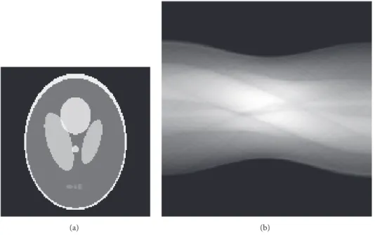
We used a modified Shepp-Logan phantom image
con-sisting of𝑒 ∈ 𝑅𝐽+shown in Figure 1(a), which is composed of
128 × 128 pixels (𝐽 = 16, 384). The projection 𝑦 ∈ 𝑅𝐼
+ was
(a) (b)
Figure 1: (a) Phantom image and (b) sinogram with noisy projection.
the white Gaussian noise such that the signal-to-noise ratio (SNR) was 30 dB unless otherwise specified and by setting the number of view angles and detector bins to 180 and 184, respectively (𝐼 = 33, 120), as illustrated in Figure 1(b) for-matted into a sinogram. A standard MATLAB (MathWorks, Natick, USA) ODE solver ode113 implementing a variable step-size variable order Adams-Bashforth-Moulton method was used for a numerical calculation of solving an initial value problem of the differential equation in (9).
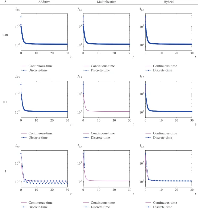
Let us first consider which is the most robust discretiza-tion method for numerical approximadiscretiza-tion. Figure 2 shows
the time course of the objective function𝐽𝛼(𝑥(𝑡)) with 𝛼 =
0.5, which we denote as 𝐽0.5(𝑥(𝑡)), for the continuous-time
system with𝛼 = 0.5 at 𝑡 and the discrete-time systems at
𝑡 = 𝛿𝑛, which are discretizations of the differential equation using the additive, multiplicative, and hybrid Euler methods
with the fixed step sizes𝛿 of 0.01, 0.1, and 1. We see that the
hybrid Euler discretization gives a similar good convergence to that of a continuous-time system; however, in the case 𝛿 = 1, the additive Euler method causes, as time goes on, an error with oscillation and solutions using the multiplicative method divergence.
Next, we consider the property of the SKLD algorithm compared with the algorithms using the ML-EM method and
MART. Note that the iterative formula in (6) with𝛿 = 1
becomes the ML-EM, SKLD, and MART algorithms when
the parameter𝛼 is equal to 0, 0.5, and 1, respectively. The
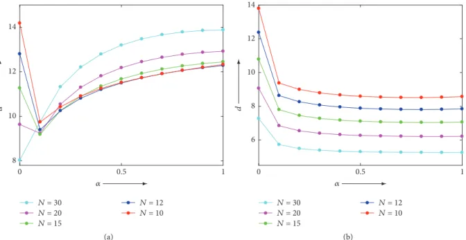
values of the root mean squared (RMS) distance or𝐿2-norm
of difference between the phantom image 𝑒 and iterative
state 𝑧(𝑁) obtained using the formula in (6) at the 𝑁th
iteration starting from the common initial value 𝑧𝑗(0) =
∑𝐼𝑖=1𝑦𝑖/ ∑𝐼𝑖=1∑𝐽𝑗=1𝐴𝑖𝑗, 𝑗 = 1, 2, . . . , 𝐽, and variations in
the parameter𝛼 are plotted in Figure 3(a). We observed a
value of𝛼 exists in the open interval (0, 1) minimizing the
quantitative measure when the number𝑁 is relatively small.
In particular, the measure of SKLD is less than those of
ML-EM and MART at, e.g., 𝑁 = 10 and 12. The presence of
noise is required for this property, which is supported by the fact that an experiment from another simulation with noise-free projection data gave different results, as shown in Figure 3(b), such that we had the minimum value of the
measure at𝛼 = 1. This was due to characteristics of the
ML-EM and MART algorithms being disadvantageous. As a result of these characteristics, ML-EM has a slow convergence [28– 31], which means that a relatively large number of iterations is required to obtain an acceptable value of the objective function, and MART is more susceptible to noise [32, 33], which may result in an increase of the convergence rate with increasing iterative steps due to the noisy projection, as
typically seen at𝛼 = 0 and 1 in Figure 3, respectively.
We carried out other experiments to examine whether
there exists an𝛼 not equal to 0 or 1, in which the value of
an objective function obtained by using the algorithm in (6)
with𝛿 = 1 takes a minimum. A set of SPECT projection data
from a publicly accessible database [34] was examined first. The sinogram of a brain scan and an image reconstructed by the SKLD algorithm are shown in Figure 4, where the number
of projections and pixels of the image are, respectively,𝐼 =
7, 680 (128 acquisition bins and 60 projection directions in
180 degrees) and𝐽 = 7, 569 (87 × 87 pixels). The projection
data for the second example were acquired from an X-ray CT scanner (Toshiba Medical Systems, Tochigi, Japan) with a body phantom [35] (Kyoto Kagaku, Kyoto, Japan) using a tube voltage of 120 kVp and a tube current of 300 mA.
Figure 5 represents the sinogram with 𝐼 = 86, 130 (957
acquisition bins and 90 projection directions in 180 degrees)
and a reconstructed image with𝐽 = 454, 276 (674 × 674
pixels). The value of the objective function𝐽0.5for the image
Additive Multiplicative Hybrid 0.01 0 10 20 30 t 103 102 J0.5 Continuous-time Discrete-time 0.1 0 10 20 30 t 103 102 J0.5 Continuous-time Discrete-time 1 0 10 20 30 t 103 102 J0.5 Continuous-time Discrete-time 0 10 20 30 t 103 102 J0.5 Continuous-time Discrete-time 0 10 20 30 t 103 102 J0.5 Continuous-time Discrete-time 0 10 20 30 t 103 102 J0.5 Continuous-time Discrete-time 0 10 20 30 t 103 102 J0.5 Continuous-time Discrete-time 0 10 20 30 t 103 102 J0.5 Continuous-time Discrete-time 0 10 20 30 t 103 102 J0.5 Continuous-time Discrete-time
Figure 2: Time course of𝐽0.5(𝑥(𝑡)) as a function of t for continuous-time (magenta) and discrete-time (blue) systems using additive, multiplicative, and hybrid Euler methods with𝛿 = 0.01, 0.1, and 1.
104, which is less than4.61 × 104obtained using FBP with a
Shepp-Logan filter.
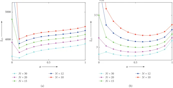
In the physical experiments, as well as a feature of the object to be reconstructed and also an overdetermined or underdetermined inverse problem, there exists a nonempty
set of the iteration number𝑁 and the parameter 𝛼 ∈ (0, 1)
(or especially𝛼 = 0.5) in which there is a minimum value
of the objective function 𝐽0.5 as shown in Figure 6. From
Figure 6(a), we observe that the algorithm with 𝛼 ≥0.1
sufficiently converges to a local minimum at a small iter-ation number, whereas the ML-EM algorithm has a slow convergence rate when the state variable is far away from the local minimum in the state space. Considering the noisy nature of the measured projection and large datasets required for reconstructing large sized images in clinical X-ray CT, the conditions suitable for practical use include a relatively small number of iterations exclusively used in IR systems [36] under which our IR method is effective, as seen in Figure 6(b).
d 1 0 0.5 8 10 12 14 N = 30 N = 20 N = 12 N = 10 N = 15 (a) d 1 0 0.5 8 6 10 12 14 N = 30 N = 20 N = 12 N = 10 N = 15 (b)
Figure 3: Values of RMS distance𝑑 using proposed algorithm in (6) at Nth iteration while varying 𝛼 with (a) noisy and (b) noise-free projections.
(a) (b)
Figure 4: (a) Sinogram and (b) reconstructed image using SKLD algorithm at 30th iteration in SPECT example.
5. Concluding Remarks
We proposed the IR algorithm based on the minimization
of𝛼-skew 𝐽-divergence between the measured and forward
projections. The objective functions to be minimized with iterative process are KL(𝑦, 𝐴𝑧), KL(𝐴𝑧, 𝑦), and 𝐽-divergence
after setting the value of parameter 𝛼 to 0, 1, and 0.5 in
the IR algorithm, respectively. We used Lyapunov’s theorem to construct a differential equation for which the IR algo-rithm is equivalent to the hybrid Euler discretization and demonstrated the monotonically decreasing convergence of
the 𝐽-divergence with iterative steps to a desired solution
of the continuous-time system. The hybrid Euler was found to have more robust performance than the additive and
(a) (b)
Figure 5: (a) Sinogram and (b) reconstructed image using SKLD algorithm at 30th iteration in X-ray CT example.
4000 5000 J0.5 1 0 0.5 N = 30 N = 20 N = 12 N = 10 N = 15 (a) 3 3.5 ×10⁴ J0.5 1 0 0.5 N = 30 N = 20 N = 12 N = 10 N = 15 (b)
Figure 6: Values of𝐽0.5using proposed algorithm in (6) at Nth iteration while varying𝛼 in (a) SPECT and (b) X-ray CT examples.
multiplicative Euler methods. The numerical and physical experiments revealed that the SKLD method is advantageous with respect to the minimization of a distance measure when the projection data are noisy and when the maximum
iteration number is relatively small. Further investigation is required to clarify the performance of the proposed IR algorithm from the viewpoint of image quality and noise evaluation.
Data Availability
The data used to support the findings of this study are available from the corresponding author upon reasonable request.
Conflicts of Interest
The authors declare no conflicts of interest regarding the publication of this paper.
Acknowledgments
This research was partially supported by JSPS KAKENHI Grant no. 18K04169.
References
[1] R. Gordon, R. Bender, and G. T. Herman, “Algebraic recon-struction techniques (ART) for three-dimensional electron microscopy and X-ray photography,” Journal of Theoretical
Biology, vol. 29, no. 3, pp. 471–481, 1970.
[2] A. C. Kak and M. Slaney, Principles of Computerized
Tomo-graphic Imaging, IEEE Service Center, Piscataway, NJ, USA,
1988.
[3] H. Stark, Ed., Image Recorvery Theory and Application, Aca-demic Press, Orlando, Fla, USA, 1987.
[4] L. A. Shepp and Y. Vardi, “Maximum likelihood reconstruction for emission tomography,” IEEE Transactions on Medical
Imag-ing, vol. 1, no. 2, pp. 113–122, 1982.
[5] S. Kullback and R. A. Leibler, “On information and sufficiency,”
Annals of Mathematical Statistics, vol. 22, no. 1, pp. 79–86, 1951.
[6] C. L. Byrne, “Iterative image reconstruction algorithms based on cross-entropy minimization,” IEEE Transactions on Image
Processing, vol. 2, no. 1, pp. 96–103, 1993.
[7] J. N. Darroch and D. Ratcliff, “Generalized iterative scaling for log-linear models,” Annals of Mathematical Statistics, vol. 43, no. 5, pp. 1470–1480, 1972.
[8] P. Schmidlin, “Iterative separation of sections in tomographic scintigrams.,” Nuklearmedizin / Nuclear Medicine, vol. 11, no. 1, pp. 1–16, 1972.
[9] C. Badea and R. Gordon, “Experiments with the nonlinear and chaotic behaviour of the multiplicative algebraic reconstruc-tion technique (MART) algorithm for computed tomography,”
Physics in Medicine and Biology, vol. 49, no. 8, pp. 1455–1474,
2004.
[10] C. Byrne, “A unified treatment of some iterative algorithms in signal processing and image reconstruction,” Inverse Problems, vol. 20, no. 1, pp. 103–120, 2004.
[11] H. Jeffreys, Theory of Probability, Oxford University Press, Oxford, 1939.
[12] H. Jeffreys, “An invariant form for the prior probability in esti-mation problems,” Proceedings of the Royal Society of London.
Series A, Mathematical and Physical Sciences, vol. 186, no. 1007,
pp. 453–461, 1946.
[13] J. Lin, “Divergence measures based on the Shannon entropy,”
IEEE Transactions on Information Theory, vol. 37, no. 1, pp. 145–
151, 1991.
[14] G. E. Crooks, “Inequalities between the Jensen-Shannon and Jeffreys divergences,” Technical Note, vol. 004, 2008.
[15] J. Schropp, “Using dynamical systems methods to solve mini-mization problems,” Applied Numerical Mathematics, vol. 18, no. 1-3, pp. 321–335, 1995.
[16] R. G. Airapetyan, A. G. Ramm, and A. B. Smirnova, “Continu-ous analog of the Gauss-Newton method,” Mathematical Models
and Methods in Applied Sciences, vol. 9, no. 3, pp. 463–474, 1999.
[17] R. G. Airapetyan and A. G. Ramm, “Dynamical systems and discrete methods for solving nonlinear ill-posed problems,” in
Applied mathematics reviews, G. A. Anastassiou, Ed., vol. 1,
pp. 491–536, World Scientific Publishing Company, Singapore, 2000.
[18] R. G. Airapetyan, A. G. Ramm, and A. B. Smirnova, “Con-tinuous methods for solving nonlinear ill-posed problems,” in
Operator theory and its applications, A. G. Ramm, Shivakumar
P. N., and A. V. Strauss, Eds., vol. 25 of Fields Inst Comm, pp. 111–136, American Mathematical Society, Providence, RI, USA, 2000.
[19] A. G. Ramm, “Dynamical systems method for solving operator equations,” Communications in Nonlinear Science and
Numeri-cal Simulation, vol. 9, no. 4, pp. 383–402, 2004.
[20] L. Li and B. Han, “A dynamical system method for solving nonlinear ill-posed problems,” Applied Mathematics and
Com-putation, vol. 197, no. 1, pp. 399–406, 2008.
[21] A. M. Lyapunov, Stability of Motion, Academic Press, New York, NY, USA, 1966.
[22] K. Fujimoto, O. Abou Al-Ola, and T. Yoshinaga, “Continuous-time image reconstruction using differential equations for computed tomography,” Communications in Nonlinear Science
and Numerical Simulation, vol. 15, no. 6, pp. 1648–1654, 2010.
[23] O. M. Abou Al-Ola, K. Fujimoto, and T. Yoshinaga, “Common Lyapunov Function Based on Kullback–Leibler Divergence for a Switched Nonlinear System,” Mathematical Problems in
Engineering, vol. 2011, pp. 1–12, 2011.
[24] Y. Yamaguchi, K. Fujimoto, O. M. Abou Al-Ola, and T. Yoshinaga, “Continuous-time image reconstruction for binary tomography,” Communications in Nonlinear Science and
Numer-ical Simulation, vol. 18, no. 8, pp. 2081–2087, 2013.
[25] K. Tateishi, Y. Yamaguchi, O. M. Abou Al-Ola, and T. Yoshinaga, “Continuous Analog of Accelerated OS-EM Algorithm for Computed Tomography,” Mathematical Problems in
Engineer-ing, vol. 2017, pp. 1–8, 2017.
[26] D. Aniszewska, “Multiplicative Runge-Kutta methods,”
Nonlin-ear Dynamics, vol. 50, no. 1-2, pp. 265–272, 2007.
[27] A. E. Bashirov, E. M. Kurpınar, and A. Ozyapıcı, “Multiplicative calculus and its applications,” Journal of Mathematical Analysis
and Applications, vol. 337, no. 1, pp. 36–48, 2008.
[28] H. M. Hudson and R. S. Larkin, “Accelerated image reconstruc-tion using ordered subsets of projecreconstruc-tion data,” IEEE
Transac-tions on Medical Imaging, vol. 13, no. 4, pp. 601–609, 1994.
[29] J. A. Fessler and A. O. Hero, “Penalized Maximum-Likelihood Image Reconstruction Using Space-Alternating Generalized EM Algorithms,” IEEE Transactions on Image Processing, vol. 4, no. 10, pp. 1417–1429, 1995.
[30] C. L. Byrne, “Accelerating the EMML algorithm and related iterative algorithms by rescaled block-iterative methods,” IEEE
Transactions on Image Processing, vol. 7, no. 1, pp. 100–109, 1998.
[31] D. Hwang and G. L. Zeng, “Convergence study of an accelerated ML-EM algorithm using bigger step size,” Physics in Medicine
and Biology, vol. 51, no. 2, pp. 237–252, 2006.
[32] B. Gustavsson, “Tomographic inversion for ALIS noise and resolution,” Journal of Geophysical Research: Space Physics, vol. 103, no. 11, pp. 26621–26632, 1998.
[33] W. Jiang and X. Zhang, “Relaxation Factor Optimization for Common Iterative Algorithms in Optical Computed Tomogra-phy,” Mathematical Problems in Engineering, vol. 2017, pp. 1–8, 2017.
[34] I. Castiglioni, I. Buvat, G. Rizzo, M. C. Gilardi, J. Feuardent, and F. Fazio, “A publicly accessible Monte Carlo database for validation purposes in emission tomography,” European Journal
of Nuclear Medicine and Molecular Imaging, vol. 32, no. 10, pp.
1234–1239, 2005.
[35] Kyoto Kagaku Co., Ltd., “CT Whole Body Phantom PBU-60,” https://www.kyotokagaku.com/products/detail03/ph-2b.html. [36] L. L. Geyer, U. J. Schoepf, F. G. Meinel et al., “State of the art:
iterative CT reconstruction techniques,” Radiology, vol. 276, no. 2, pp. 339–357, 2015.
Hindawi www.hindawi.com Volume 2018
Mathematics
Journal of Hindawi www.hindawi.com Volume 2018 Mathematical Problems in Engineering Applied Mathematics Hindawi www.hindawi.com Volume 2018Probability and Statistics Hindawi
www.hindawi.com Volume 2018
Hindawi
www.hindawi.com Volume 2018
Mathematical PhysicsAdvances in
Complex Analysis
Journal ofHindawi www.hindawi.com Volume 2018
Optimization
Journal of Hindawi www.hindawi.com Volume 2018 Hindawi www.hindawi.com Volume 2018 Engineering Mathematics International Journal of Hindawi www.hindawi.com Volume 2018 Operations Research Journal of Hindawi www.hindawi.com Volume 2018Function Spaces
Abstract and Applied Analysis Hindawi www.hindawi.com Volume 2018 International Journal of Mathematics and Mathematical Sciences Hindawi www.hindawi.com Volume 2018Hindawi Publishing Corporation
http://www.hindawi.com Volume 2013 Hindawi www.hindawi.com
World Journal
Volume 2018 Hindawiwww.hindawi.com Volume 2018Volume 2018