INVITED PAPER
Special Section on Coding and Coding Theory-Based Signal Processing for Wireless CommunicationsSpatially Coupled LDPC Coding and Linear Precoding for MIMO Systems ∗
Zhonghao ZHANG†a), Chongbin XU†,andLi PING†,Nonmembers
SUMMARY In this paper, we present a transmission scheme for a multiple-input multiple-output (MIMO) quasi-static fading channel with imperfect channel state information at the transmitter (CSIT). In this scheme, we develop a precoder structure to exploit the available CSIT and apply spatial coupling for further performance enhancement. We derive an analytical evaluation method based on extrinsic information transfer (EXIT) functions, which provides convenience for our precoder design.
Furthermore, we observe an area property indicating that, for a spatially coupled system, the iterative receiver can perform error-free decoding even the original uncoupled system has multiple fixed points in its EXIT chart.
This observation implies that spatial coupling is useful to alleviate the un- certainty in CSIT which causes difficulty in designing LDPC code based on the EXIT curve matching technique. Numerical results are presented, showing an excellent performance of the proposed scheme in MIMO fading channels with imperfect CSIT.
key words: spatial coupling, linear precoding, MIMO, LDPC code, linear minimum mean-square error, message passing detection, EXIT chart
1. Introduction
The extrinsic information transfer (EXIT) chart analysis technique [1]–[5] has been widely used for the design of low-density parity-check (LDPC) codes and turbo codes with iterative decoding [6]–[8]. With this technique, near capacity performance can be approached by matching the EXIT curves of two local processors (decoders) of an iter- ative receiver in an additive white Gaussian noise (AWGN) channel [3], [5].
For a multiple-input multiple-output (MIMO) system with perfect channel state information at the transmitter (CSIT), the channel can be transformed into a set of paral- lel subchannels using singular value decomposition (SVD).
The MIMO capacity can then be achieved by independent coding for each sub-channel, following the water-filling principle [9]. The design problem in this case is similar to that for an AWGN channel.
For aquasi-staticMIMO channel without CSIT, how- ever, the optimal design for the transmitter remains a chal- lenging problem. In this case, it is difficult to apply the EXIT curve matching technique. (See Fig. 5 for this issue.)
Manuscript received July 6, 2012.
Manuscript revised August 22, 2012.
†The authors are with the Department of Electronic Engineer- ing, City University of Hong Kong, Hong Kong SAR, P.R. China.
∗This work has been performed in the framework of the FP7 project ICT-248894 WHERE2 (Wireless Hybrid Enhanced Mobile Radio Estimators-Phase 2) which is partly funded by the European Union.
a) E-mail: [email protected] DOI: 10.1587/transcom.E95.B.3663
This problem becomes more complicated when the avail- able CSIT is imperfect, containing both useful information as well as errors. In this case, to the best of our knowledge, even the outage capacity of the system is still unknown and the optimal transmitter design problem remains open [10].
Detection complexity is another issue, especially for MIMO systems with a large number of antennas.
Among different options, linear minimum mean-square er- ror (LMMSE) [11] detection has suboptimal performance but relatively low complexity. Techniques that can improve the performance of MIMO systems with LMMSE detection are thus highly desirable.
In this paper, we will first consider the transmission is- sues for MIMO systems without CSIT. We focus on a linear precoding technique that can facilitate LMMSE detection.
We develop an analytical EXIT curve method to evaluate the performance of MIMO systems with LDPC coding and linear precoding. We apply the spatial coupling approach [12]–[14] to treat the EXIT curve mismatching problem. We show that, with spatial coupling, an iterative decoder can converge to the correct detection even when the two EXIT curves have multiple fixed points. This leads to a noticeable performance improvement.
We will then extend our discussions to MIMO systems with partial (imperfect) CSIT. We propose a heuristic pre- coding scheme that works efficiently with partial CSIT. Spa- tial coupling is again used to deal with the EXIT curve mis- matching problem. Numerical results demonstrate that the proposed scheme can achieve impressive gain (relative to the case of no CSIT). This provides an attractive solution to practical MIMO systems.
2. System Model
Consider a flat-fading MIMO system withMRreceive anten- nas andMTtransmit antennas. Denote byH(n) theMR×MT
channel matrix andy(n) the transmitted sequence of length MT at time slotn. The received sequence of length MR is given by
r(n)=H(n)y(n)+z(n) (1) wherez(n) denotes a complex AWGN sequence of length MRwith zero mean and covariance matrixN0I.
For convenience of the discussion, we consider the fol- lowing extended system model overNtime slots
r=Hy+z (2)
Copyright c2012 The Institute of Electronics, Information and Communication Engineers
whereHis anN MR×N MT block diagonal matrix withN diagonal submatrices, i.e.,
H=diag (H(1), . . . ,H(N)) (3) andyis a length-NMTtransmitted sequence
y=
yT(1), . . . ,yT(N)T
. (4)
The other sequencesrandzare defined similarly.
To make the discussion simpler, we assume that the channel is time-invariant overNtime slots, i.e.,H(n)=H for 1≤ n ≤ N. The extension to the time-varying fading case is straightforward.
To characterize the CSIT, we consider the following channel mean information (CMI) model [10], [15]
H= √
αH+√
1−αHW (5)
whereHandHW areN MR ×N MT block diagonal matri- ces, representing the known and unknown parts of H at the transmitter. The entries of the diagonal submatrices of HWare modeled as independent and identically distributed (i.i.d.) complex Gaussian random variables with zero mean and unit variance. The CSIT quality is measured by α (0 ≤ α ≤ 1): α =0 for no CSIT and α=1 for perfect CSIT.
For simplicity, we first discuss the no CSIT case (α= 0) in Sects. 3, 4, and 5, and then discuss the precoder design in the partial CSIT case (α >0) in Sect. 6.
3. Transmitter and Receiver Structure
3.1 Linear Precoding without CSIT
Figure 1(a) illustrates the transmitter structure and the chan- nel, whereyis generated by a linear precoder as
y=Px. (6)
HerePdenotes anN MT×N MT precoding matrix andxis a symbol sequence of lengthNMT generated by an LDPC encoder. The power of each symbol is assumed to be nor- malized.
Without CSIT (i.e.,α=0), we adopt the following lin- ear precoder structure developed in [16]
P=ΠF (7)
whereΠandFare, respectively, anNMT ×NMT random permutation matrix and anNMT×NMT Hadamard matrix.
This precoder structure provides diversity advantage [16].
Denote byA=HPthe equivalentNMR×NMTchannel matrix. From (2) and (6), we have
r=Ax+z. (8)
Figure 1(b) illustrates a factor graph representation [17], [18] of the block diagram in Fig. 1(a), where each cir- cle represents a variable node and each square represents a check node.
Fig. 1 (a) Transmitter structure. (b) Factor graph of the transmitter. (c) A concise form of the factor graph in (b).
Figure 1(b) can be redrawn in a more concise form as shown in Fig. 1(c), where each node (a double circle or a double square) represents multiple nodes in Fig. 1(b). Ac- cordingly, each edge in Fig. 1(c) represents multiple edges in Fig. 1(b). This concise factor graph provides convenience for our discussions below.
3.2 Message Passing Detection Algorithm
The symbol sequencexin Fig. 1(c) satisfies two constraints which are imposed, respectively, by the linear system in (8) and by the LDPC code.
At the receiver, message passing detection algorithm [17], [18] is adopted based on the above two constraints.
This is illustrated in Fig. 1(c), where the concise factor graph represents the receiver structure. There are three local de- tectors, namely, an LMMSE detector, a variable node detec- tor (VND), and a check node detector (CND). The LMMSE detector recovers the symbol sequencex based on the lin- ear constraint in (8), while the CND and VND decode the symbol sequencex based on the LDPC coding constraint.
They exchange messages following the turbo principle [8] as shown in Fig. 1(c), where each message is a sequence con- sisting of log-likelihood ratios (LLRs). We use superscripts to distinguish these messages. For example, the message from the LMMSE detector to the VND is denoted byξLV. The other three messages are distinguished similarly.
3.3 LMMSE Detection
For convenience, we assume binary phase shift keying (BPSK) [19] for the coded symbols inx. The discussion can be extended to other modulation methods [20].
Assume that the LLR messageξVL ={ξVLm }of length
NMThas been generated and passed to the LMMSE detector as shown in Fig. 1(c). (We will return to this issue in 3.5.) We can generate the LMMSE detection outputsξLV={ξmLV} of lengthNMTas follows.
Compute thea priorimean and variance ofxmas [21]
xm=tanh(ξmVL/2) andvm=1−x2m. (9) Letting
vm≈v= 1 N MT
N MT
n=1
vn (10)
we can obtain the LMMSE estimate ofxas [11]
ˆ
x=x+vAHR−1(r−Ax) (11) wherex={xm}, andR=vA AH+N0I.
TheextrinsicLLR ofxmis given by (see Appendix) ξLVm =2
Ω−m1,mxˆm−v−1xm
(12)
whereΩm,m is them-th diagonal entry of the mean-square error (MSE) matrix [11]
Ω=vI−v2AHR−1A. (13) We write the LMMSE detection outputs asξLV={ξLVm }, which are passed to the VND as shown in Fig. 1(c).
3.4 Modeling the LMMSE Detection Outputs
The LMMSE detection outputs can be modeled as the ob- servations from an equivalent AWGN channel. It is shown that when the precoder matrixFin (7) is properly chosen, ξmLVcan be expressed as [c.f., (5), (17) and (18) in 21]
ξLVm =μxm+εm (14)
whereμis a constant with respect tom, andεmis an indepen- dent Gaussian random variable with zero mean and variance σ2.
Define the signal-to-noise ratio (SNR) for (14) asρLV≡ μ2/σ2. We have [c.f., (16c) in 16]
ρLV=φ(v)≡
⎛⎜⎜⎜⎜⎜
⎝ 1 N MT
trace 1
vI+AHA N0
−1⎞
⎟⎟⎟⎟⎟
⎠
−1
−1
v. (15) 3.5 VND/CND Operations and Overall Iterative Process Based on (14), we can regard the LMMSE detection outputs as the observations from an equivalent AWGN channel. The messagesξVCandξCVbetween the CND and VND are gen- erated based on the standard message passing algorithm [4], [5]. The details are omitted here. Furthermore, the message ξVL={ξmVL}is generated by the VND as
ξVLm =
n
ξCVn (16)
where the subscriptnrepresents the edge index and the sum
is over all edges connected to the variable nodem. The mes- sageξVLis then used to refine the LMMSE detection outputs in the next iteration (see (9)).
With the above schedule, the messagesξLV,ξVC,ξCV, andξVLare updated in sequence during each iteration. The iterative detection continues until convergence. This sched- ule is also adopted in [14].
4. Performance Analysis based on EXIT Charts
4.1 Modeling LLR with i.i.d. Gaussian Assumption Following [2], [4], we assume that the LLRs in each mes- sage in Fig. 1(c) are i.i.d. Gaussian random variables, satis- fying the consistency condition [2]. By doing this, a mes- sage can be characterized by the individual statistics of each entry.
Letξbe an LLR in a message andxthe corresponding BPSK signal. Under the above assumption,ξcan be mod- eled as [c.f., (9), (10) in 2]
ξ=(σ2/2)x+σε (17)
whereεis an independent Gaussian random variable with zero mean and unit variance. The mutual information be- tweenxandξis given by [2]
I=J(σ)≡1−
+∞
−∞
e−(t−σ2/2)2/2σ2
√2πσ log2(1+e−t)dt. (18) With (18), we can compute the mutual information for every message in Fig. 1(c) under the i.i.d. Gaussian assump- tion. This is shown in Fig. 2, where the superscripts are used to indicate the corresponding relationship between the mu- tual information and the messages. For example,ILVcorre- sponds toξLV.
Following [2] and [4], we adopt the so-called EXIT functions to characterize the behavior of these local detec- tors, as discussed in the next three subsections.
4.2 Characterization of the LMMSE Detector
LetILV=χ(IVL) be the EXIT function of the LMMSE de- tector. It can be derived as follows.
From (15), we have ILV=J(σLV)=J(2
ρLV)=J(2
φ(v)) (19)
where the first equality follows from (18) and second equal- ity follows from (17) in [21].
Combining (9) and (10), and lettingN → ∞, we have
Fig. 2 Mutual information characterization for Fig. 1(c).
v=1− 1 N MT
N MT
n=1
tanh2(ξVLn /2) (20a)
→1− +∞
−∞
e−t2/2
√2π tanh2
(σVL)2 4 +σVL
2 t
dt (20b)
≡T(σVL) (20c)
where (20b) follows from the model in (17), and σVL in (20c) is given by (usingJ(·) in (18))
σVL=J−1(IVL). (21)
Combining (19), (20) and (21), forN→ ∞, we have ILV=χ(IVL)≡J
2
φ
T
J−1(IVL)
. (22)
The analytic form of the EXIT function in (22) pro- vides conventions for our precoder design as to be discussed in 6.3.
4.3 Characterization of the VND and CND
The EXIT functions for the VND and CND are denoted by (see Fig. 2)
IVC=λ(ICV,ILV), IVL=η(ICV), andICV=g(IVC). (23) These EXIT functions are determined by the degree distributions of an LDPC code [4]. For a (dl, dr) regular LDPC code, we have
λ(ICV,ILV)≡J
(dl−1)
J−1(ICV)2+
J−1(ILV)2
(24) η(ICV)≡J dlJ−1(ICV)
(25) g(IVC)≡1−J
(dr−1)−1J−1(1−IVC)
. (26)
4.4 EXIT Chart Analysis
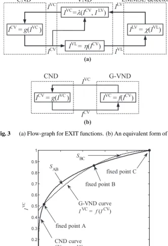
The flow-graph in Fig. 3(a) summarizes the EXIT functions in (22), (24), (25) and (26). We can combine the VND and LMMSE detector in Fig. 3(a) into an overall functional block, as marked by “G-VND” (standing for generalized VND) in Fig. 3(b). The latter involves two EXIT functions, namelyg(·) in (26) and
f(ICV)≡λ ICV, χ
η(ICV)
. (27)
Based on Fig. 3(b), we can predict the performance of the iterative receiver as follows. Denote by the subscript “q”
the iteration number. We initializeI0CV=0, which implies noa prioriinformation from the CND to the G-VND at the beginning of the iterative detection process. The mutual in- formation during the iterative process can be tracked as
IqVC= f(IqCV−1), andIqCV=g(IVCq )q=1, . . . ,Q. (28) At the end of the iterative process,IQVCandIQCVare used to predict the bit error rate (BER) and frame error rate (FER)
Fig. 3 (a) Flow-graph for EXIT functions. (b) An equivalent form of (a).
Fig. 4 An EXIT chart with three fixed points.
performance [2], [16], [21].
The behavior of the iterative process in (28) can be demonstrated by an EXIT chart as shown in Fig. 4. It is wanted that the iterative process converges to ICV =1 and IVC=1, (i.e., point C in Fig. 4), which represents error free detection. However, there can be multiple fixed points in an EXIT chart, such as the example with three fixed points labeled by “A”, “B” and “C” in Fig. 4. In this case, the iter- ative process will converge to the first fixed point, i.e., point A in Fig. 4. This indicates potential detection error. We will return to this issue later in 5.3.
We can increase the transmit power to avoid the situ- ation of multiple fixed points. However, this incurs loss in power efficiency.
4.5 Mismatch between EXIT Curves
It has been shown that near capacity performance can be achieved if the following matching condition is fulfilled [3], [20], [22]
f(ICV)=g−1(ICV) 0≤ICV≤1 (29) whereg−1(·) is the inverse function ofg(·).
Fig. 5 An EXIT chart for 10 channel realizations.
In (29), g(·) is determined by the check node degree distribution of an LDPC code (see (26)) but f(·) is deter- mined by the variable node degree distribution of an LDPC code as well as the channel (see (15), (23), (24), (25) and (27)).
In the case of full CSIT, we can design the precoder ac- cording to the matching condition in (29) as to be discussed in 6.1. Alternatively, we can also tune the degree distribu- tions of the LDPC codes [3], [5], [20]. Both methods lead to excellent performance.
Without perfect CSIT, the matching condition in (29) cannot be satisfied by optimizing the degree distributions of the LDPC code or the precoder structure. This is because, as mentioned above,f(·) is a function of the channel matrixH, as illustrated in Fig. 5. Here, the EXIT curves are generated using a (3, 6) LDPC code and 10 random realizations of a 2×2 MIMO Rayleigh fading channel. For different channel realizations, f(·) varies noticeably whileg(·) remains fixed as discussed above. This clearly demonstrates the main dif- ficulty in meeting the matching condition in (29): without accurate CSIT, f(·) is uncertain at the transmitter. This mis- matching problem may lead to noticeable performance loss.
5. Spatial Coupling
5.1 Spatial Coupling Principle
In this section, we adopt the spatial coupling approach pro- posed in [13] to mitigate the mismatching problem as men- tioned in 4.5.
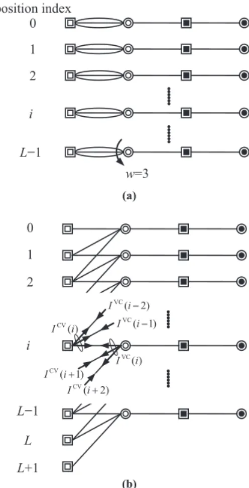
The basic principle of spatial coupling is illustrated in Fig. 6. Due to space limitation, our discussion below is very brief. For details, please refer to [13].
In Fig. 6(a), we create Lparallel copies of the system in Fig. 1(c). Each copy is referred to as a “position”. At each position, the edges between the check nodes and the variable nodes are randomly and uniformly divided intow edge subsets (w < L) indexed byk, k=0, . . . ,w−1. In Fig. 6(a),w =3 and each edge subset is represented by a line between the white double circle and the white double
Fig. 6 Spatial coupling principle. (a) Edge grouping. (b) Edge reconnection and mutual information characterization.
square. Note that the variable nodes are only connected to the check nodes at the same position in Fig. 6(a).
In Fig. 6(b), we perform spatial coupling as follows.
The variable nodes at each positioniare reconnected to the check nodes atwpositions (fromitoi+w−1) throughw edge groups, respectively. Extra check nodes are created at w−1 positions for spatial coupling termination. This results in the factor graph of a spatially coupled LDPC (SC-LDPC) code.
Assume that a (dl, dr) regular LDPC code is used at each position. The resultant spatially coupled LDPC code is referred to as a (dl,dr,L,w) SC-LDPC code [13].
It has been demonstrated that SC-LDPC codes can achieve excellent performance in nonfading channels. See [12]–[14] and references therein. In what follows, we will show that SC-LDPC codes can be used in fading MIMO channels to handle the EXIT curve mismatching problem discussed in 4.5.
The message passing detection algorithm for the SC- LDPC coded MIMO system can be carried out using the factor graph in Fig. 6(b) in a straightforward way.
5.2 EXIT Chart Analysis for a Spatially Coupled System The EXIT chart analysis technique can be extended to the spatially coupled system in Fig. 6(b). Let us focus on posi-
tioniin Fig. 6(b). Here the mutual informations are indexed by the position number, i.e.,ICV(i) andIVC(i).
The nodes in Fig. 6(b) can still be characterized byg(·) andf(·) in (26) and (27). The key point is that each incom- ing message is a uniform mixture of LLRs from different po- sitions with different mutual information values (see Fig. 6).
We can thus use the average mutual information to charac- terize the incoming messages. For the G-VND and CND at positioni, the input average mutual informations are given by
1 w
w−1
k=0
ICV(i+k), and 1 w
w−1
k=0
IVC(i−k). (30) Following [13], we impose boundary constraintsIVC(i)=1 fori<0 ori≥L. Based on (26), (27) and (30), we have
IVC(i)= f
⎛⎜⎜⎜⎜⎜
⎜⎝1 w
w−1
k=0
ICV(i+k)
⎞⎟⎟⎟⎟⎟
⎟⎠ (31)
ICV(i)=g
⎛⎜⎜⎜⎜⎜
⎜⎝1 w
w−1
k=0
IVC(i−k)
⎞⎟⎟⎟⎟⎟
⎟⎠. (32)
Again, denote byqthe iteration number. We initialize I0CV(i)=0, for 0≤i<L+w−1. For 1≤q ≤Q, we track the mutual informations during the iterative process as
⎧⎪⎪⎪⎪⎪⎪⎪
⎪⎨⎪⎪⎪⎪⎪
⎪⎪⎪⎩
IqVC(i)=f
1 w
w−1
k=0IqCV−1(i+k)
1≤i<L IqVC(i)=1 i<0 ori≥L IqCV(i)=g
1 w
w−1 k=0
IqVC(i−k)
1≤i<L+w−1
. (33)
The results of the above recursion can be used to predict system performance.
5.3 Area Property
Assume that there are multiple fixed points in an EXIT chart for an LDPC coded system without spatial coupling. The it- erative process in (28) then converges to the first fixed point, which is not desirable as we discussed before.
With spatial coupling, interestingly, we observed that the iterative process in (33) may converge to the correct de- cision, i.e.,ICVq (i)→1 andIqVC(i)→1, even the EXIT chart for the system in each position before spatial coupling has multiple fixed points. We have conducted a large amount of experiments. We observed that forLw1,IqCV(i)→1 andIqVC(i) → 1 if SAB < SBC, whereSAB and SBC are the areas of the two regions as shown in Fig. 4. We conjec- ture that this property is true for general cases. We are now working on a rigorous proof of this conjecture.
Based on the above conjecture, we have a simple method to predict the performance of a spatially coupled system. Given a channel realization, assuming that there are only three fixed points as shown in Fig. 4, we can shift f(·) by tuning transmission powerPT. ThusSAB andSBC can be expressed as functions ofPT, i.e.,SAB(PT) andSBC(PT).
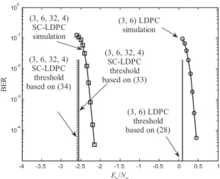
Fig. 7 BER performance and thresholds for a 2×2 fixed fading MIMO system with (3, 6) LDPC coding and (3, 6, 32, 4) SC-LDPC coding.
The value ofPTthat results in
SAB(PT)=SBC(PT) (34)
is used as the threshold for error-free performance for the given channel realization.
We use a numerical example to support the conjecture.
Consider a 2×2fixedfading MIMO system with H=
−1.749+0.927√
−1 −0.857−1.204√
−1
−0.319+0.480√
−1 −0.109−0.006√
−1
. (35) We compare the performance of a (3, 6) LDPC code and a (3, 6, 32, 4) SC-LDPC code, both with length 217. Figure 7 shows the simulated BER performance. Clearly, spatial cou- pling leads to performance gain of about 2.5 dB. The thresh- olds calculated using the EXIT functions based on (29), (33) and using the area property based on (34) are also included for comparison. Notice that the threshold based on (33) is forw=4 andL=32, while the threshold based on (34) is for Lw1. Their difference is very small, which provides a useful evidence for the conjecture.
6. Precoder Design with Perfect and Partial CSIT
6.1 Perfect CSIT Case
The discussions so far have been on systems without CSIT.
We now consider more general cases with CSIT. We first as- sume that CSIT is perfect (α=1) soHis accurately known at the transmitter. Following [16], we can modify the pre- coder in (7) to the following form
P=VW1/2ΠF (36)
whereVis the beamforming matrix obtained using the SVD H=UDVH,Wis a diagonal matrix representing power allo- cation, ΠandFare the same as those in (7). In principle, the diagonal entries of W have a water-filling effect [16].
Roughly speaking, the use ofW allocates more energy to channel directions with high gains and vise versa. An opti- mization procedure forWcan be found in [16].
6.2 Partial CSIT Case
We now consider CSIT uncertainty (α <1). Forα=0, the precoder structure in (7) is adopted. To facilitate our discus- sion below, we rewrite (7) as
P=V·I·ΠF (37)
whereVcan be an arbitrary unitary matrix. It is easy to see thatVandIin (37) will not affect the performance.
For 0 < α < 1, we do not have the optimal solution in this case, so we consider the following heuristic option.
Let the SVD ofHbeH=U DVH. We first pretend that the CSIT is perfect andH=H(i.e., we ignore the uncertain part HW.) Then the method outlined in 6.1 can be used to design a precoder structure below
P=VW1/2ΠF (38)
where two upper hyphens “−” are added onVandWto em- phasize that they are obtained using the SVD of Hrather thanH. Note thatHW is ignored in this design so the pre- coder structure in (38) may not be reliable.
On the other hand, we can also assume no CSIT and ignore the available information H. Then, again, we have the precoder in (37).
We combined the two precoders in (37) and (38) as P=V(β1I+β2W)1/2ΠF (39) whereβ1andβ2are two nonnegative weight coefficients to be optimized. Intuitively,Win (39) has the water-filling ef- fect as mentioned in 6.1, sinceHcan still provide informa- tion (though imperfect) about the channel condition. Also, the termIin (39) represents a diversity effect against CSIT uncertainty.
We obtain the weight coefficients in (39) using a two- dimensional search. The EXIT chart analysis outlined in Sect. 4 provides a fast means for this purpose.
Provided that the CSIT is imperfect, the condition in (29) cannot be guaranteed in general, thus the mismatching problem demonstrated in Fig. 5 still exists for the precoder in (39). Again, spatial coupling can be applied to treat the problem, as shown in the next subsection.
6.3 Numerical Results
We now present simulation results to demonstrate the per- formance of the precoder in (39). The simulation settings are as follows. The MIMO channel is quasi-static Rayleigh fading withMR =MT =4. The signaling method is QPSK with Gray mapping [19]. An underlying (3, 6) regular LDPC code is used with and without spatial coupling. The coding length is 217for both cases.
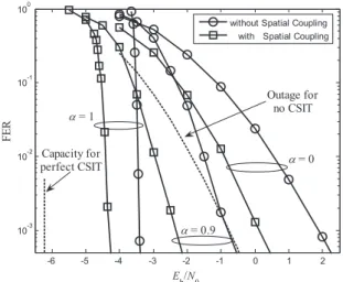
The simulated FER performance is shown in Fig. 8. In the case of no CSIT (α=0), there is a gain of about 2 dB between the systems with and without spatial coupling. This
Fig. 8 FER performance for a 4×4 Rayleigh fading MIMO system with (3, 6) LDPC coding and (3, 6, 32, 4) SC-LDPC coding.
gain is verified by EXIT chart analysis based on the area property discussed in 5.3. We can observe that there is still about 0.7 dB gap between the system with spatial coupling and the outage performance. We believe that this gap can be reduced by carefully designing the degree distributions of the SC-LDPC code.
In the case of perfect CSIT (α =1), the precoder in (39) can provide an extra gain (compared with the no CSIT case) of about 5.5 dB (at FER=10−3) for the system with- out spatial coupling and about 4.5 dB for the system with spatial coupling. We can further observe that in the perfect CSIT case, the spatial coupling gain is about 1 dB, which is less than that in the no CSIT case. Furthermore, there is a gap of about 2 dB between the system with spatial coupling and the capacity. We are seeking for a solution for further improvement.
In the case of partial CSIT (α=0.9), the precoder in (39) performs between the two extreme cases of no CSIT and perfect CSIT. Again, in this case, spatial coupling pro- vides noticeable gain.
7. Conclusions
We developed a combined scheme involving LDPC coding, linear precoding and spatial coupling. We derived an ana- lytical method to evaluate the performance based on EXIT functions. We also observed an area property for a spatially coupled system, indicating that error-free decoding can be achieved even the underlying uncoupled system has multi- ple fixed points in its EXIT chart. This property is very use- ful to alleviate the uncertainty in partial CSIT which leads to difficulty designing LDPC codes based on the EXIT curve matching technique. Numerical results show that the pro- posed scheme can achieve excellent performance in MIMO channels with partial CSIT.
References
[1] S. ten Brink, “Convergence of iterative decoding,” Electron. Lett.,
vol.35, no.10, pp.806–808, May 1999.
[2] S. ten Brink, “Convergence behavior of iteratively decoded par- allel concatenated codes,” IEEE Trans. Commun., vol.49, no.10, pp.1727–1737, Oct. 2001.
[3] A. Ashikhmin, G. Kramer, and S. ten Brink, “Extrinsic informa- tion transfer functions: Model and erasure channel properties,” IEEE Trans. Inf. Theory, vol.50, no.11, pp.2657–2673, Nov. 2004.
[4] S. ten Brink, G. Kramer, and A. Ashikhmin, “Design of low-density parity-check codes for modulation and detection,” IEEE Trans.
Commun., vol.52, no.4, pp.670–678, April 2004.
[5] T. Richardson and R. Urbanke, Modern Coding Theory, Cambridge University Press, 2008.
[6] R.G. Gallager, “Low-density parity-check codes,” IEEE Trans. Inf.
Theory, vol.IT-8, no.1, pp.21–28, Jan. 1962.
[7] D.J.C. MacKay and R.M. Neal, “Near Shannon limit performance of low density parity check codes,” Electron. Lett., vol.32, no.18, pp.1645–1646, Aug. 1996.
[8] C. Berrou, A. Glavieux, and P. Thitimajshima, “Near Shannon limit error-correcting coding and decoding: Turbo codes,” Proc. ICC’93, pp.1064–1070, Geneva, Switzerland, May 1993.
[9] D. Tse and P. Viswanath, Fundamentals of Wireless Communica- tion, Cambridge University Press, 2005.
[10] A. Goldsmith, S.A. Jafar, N. Jindal, and S. Vishwanath, “Capacity limits of MIMO channels,” IEEE J. Sel. Areas Commun., vol.21, no.5, pp.684–702, June 2003.
[11] S.M. Kay, Fundamentals of Statistical Signal Processing: Estimation Theory, Prentice-Hall, New Jersey, 1993.
[12] A. Pusane, R. Smarandache, P. Vontobel, and J.D.J. Costello, “De- riving good LDPC convolutional codes from LDPC block codes,”
IEEE Trans. Inf. Theory, vol.55, no.6, pp.2577–2598, Feb. 2011.
[13] S. Kudekar, T. Richardson, and R. Urbanke, “Threshold satura- tion via spatial coupling: Why convolutional LDPC ensembles per- form so well over the BEC,” IEEE Trans. Inf. Theory, vol.57, no.2, pp.803–834, Feb. 2011.
[14] A. Yedla, P. Nguyen, H. Pfister, and K. Narayanan, “Spatially- coupled codes and threshold saturation on intersymbol-interference channels,” http://arxiv.org/abs/1107.3253, 2011.
[15] S. Venkatesan, S. Simon, and R. Valenzuela, “Capacity of a Gaus- sian MIMO channel with nonzero mean,” Proc. IEEE VTC., vol.3, pp.1767–1771, Oct. 2003.
[16] X. Yuan, C. Xu, L. Ping, and X. Lin, “Precoder design for multiuser MIMO ISI channels based on iterative LMMSE detection,” IEEE J.
Sel. Top. Signal Process., vol.3, no.6, pp.1118–1128, Dec. 2009.
[17] F.R. Kschischang, B.J. Frey, and H.-A. Loeliger, “Factor graphs and the sum-product algorithm,” IEEE Trans. Inf. Theory, vol.47, no.2, pp.498–519, Feb. 2001.
[18] H.-A. Loeliger, J. Dauwels, J. Hu, S. Korl, L. Ping, and F.R. Kschis- chang, “The factor graph approach to model-based signal process- ing,” Proc. IEEE, June 2007.
[19] J. Proakis, Digital Communications, 4th ed., McGraw-Hill, 2000 [20] X. Yuan, L. Ping, and A. Kavcic, “Achievable rates of coded MIMO
systems with linear precoding and iterative linear MMSE detection,”
submitted to IEEE Trans. Inf. Theory.
[21] X. Yuan, Q. Guo, X. Wang, and L. Ping, “Evolution analysis of low-cost iterative equalization in coded linear systems with cyclic prefixes,” IEEE J. Sel. Areas Commun., vol.26, no.2, pp.301–310, Feb. 2008.
[22] K. Bhattad and K.R. Narayanan, “An MSE-based transfer chart for analyzing iterative decoding schemes using a Gaussian approxima- tion,” IEEE Trans. Inf. Theory, vol.53, no.1, pp.22–38, Jan. 2007.
Appendix
In this appendix, we derive (12). Denote by am the m-th column vector ofA. TheextrinsicLLRξLVm is given by (c.f.
(4b) in [21])
ξLVm =2aHmR−1(r−Ax)+aHmR−1amxm
1−vamHR−1am
(A·1a)
=2
⎛⎜⎜⎜⎜⎝amHR−1(r−Ax) 1−vamHR−1am
+1 v
xm
1−vamHR−1am
−xm
v
⎞⎟⎟⎟⎟⎠ (A·1b)
=2
xm+vaHmR−1(r−Ax) v(1−vaHmR−1am) − xm
v
. (A·1c)
From (11) and (13), we have ˆ
xm=xm+vaHmR−1(r−Ax) (A·2) Ωm,m=v−v2amHR−1am. (A·3) Substituting (A·2) and (A·3) into (A·1c), we obtain (12).
Zhonghao Zhang received the B.S. and M.S. degrees in Electrical Engineering from University of Electronic Science and Technol- ogy of China in 2005 and 2008, respectively. He is currently pursuing the Ph.D. degree at City University of Hong Kong. His research interests span the areas of iterative detection and infor- mation theory.
Chongbin Xu received the B.E. degree from Xian Jiaotong University in 2005, and the Ph.D.
degree from the Department of Electronic Engi- neering in Tsinghua University, Beijing, China.
He is currently working at the City University of Hong Kong. His research interests include iterative detection, transceiver design of MIMO systems.
Li Ping(S’87-M’91-SM’06-F’09) received his Ph.D. degree at Glasgow University in 1990.
He lectured at Department of Electronic Engi- neering, Melbourne University, from 1990 to 1992, and worked as a research staffat Tele- com Australia Research Laboratories from 1993 to 1995. He has been with the Department of Electronic Engineering, City University of Hong Kong, since January 1996 where he is now a chair professor. Dr. Li Ping received a British Telecom — Royal Society Fellowship in 1986, the IEE J.J. Thomson premium in 1993 and a Croucher Foundation Award in 2005. He is now serving as a member of Board of Governors of IEEE Information Theory Society from 2010 to 2012 and is a fellow of IEEE. His research interests include iterative signal processing, mobile communica- tions, coding and modulation, information theory and numerical methods.