Prediction by a Set of New Features and Feature Selection with Grid Search
著者 ファボリセン ロシキンル ルンバンラジャ
著者別表示 Favorisen Rosyking Lumbanraja journal or
publication title
博士論文要旨Abstract 学位授与番号 13301甲第4627号
学位名 博士(工学)
学位授与年月日 2017‑09‑26
URL http://hdl.handle.net/2297/00049551
Creative Commons : 表示 ‑ 非営利 ‑ 改変禁止 http://creativecommons.org/licenses/by‑nc‑nd/3.0/deed.ja
A Study on the Protein Phosphorylation Site Prediction by a Set of New Features and Feature Selection with
Grid Search
Graduate School of
Natural Science & Technology Kanazawa University
Division of Electrical Engineering and Computer Science
Student ID No.: 1424042020
Name: Favorisen Rosyking Lumbanraja
Chief Advisor: Professor Kenji Satou
Date of Submission: 30 June 2017
ii
Abstract
Post-translational modification is one way of expanding genetic coding capacity to generate diversity in the corresponding proteomes. One of the most common post-translational modifications is phosphorylation. It is the process of adding a phosphate group to a target residue, which are Serine, Threonine, or Tyrosine.
Phosphorylation plays an important role in eukaryotic cell activities, such as cell cycle, signaling cell growth, and intracellular signal transduction. Research in the past has commonly conducted phosphorylation site identification using an experimental approach. One common experimental approach for identifying phosphorylation sites is by using mass spectrometry. By recording and measuring the mass of the ion sample, we can accurately identify phosphorylation sites.
However, there are disadvantages in implementing mass spectrometry. (i) It requires an expensive machine. (ii) It also requires supporting tools and materials to conduct the experiment. (iii) Preparing the sample and analyzing it are both time consuming and labor intensive. (iv) Adequate skills are required to operate the machinery and analyze the results.
Another way to identify phosphorylation sites is the computational approach. A lot of research implements this approach because of improvements in computer technology and machine learning.
In general, there are two different methods of the computational approach. The first method is kinase- specific phosphorylation site prediction. It requires information about the protein kinase, which catalyzes the process, as well as information about phosphorylated protein sites. However, information about kinase proteins for phosphorylation is often not available publicly. The second method is the non-kinase-specific phosphorylation site prediction. This method only requires the information of the phosphorylated protein to conduct a prediction.
In this research, we conducted a non-kinase-specific phosphorylation site prediction by proposing new combinations of features. Feature selection was implemented to improve the classification result. There are two types of data sets we used to implement the method. The first data set is the P.ELM data set, which contains human and several animal phosphorylation sites. The second one is the PPA data set, which we used as an independent data set. This data set contains phosphorylation site information from plants. For each data set, we classified the phosphorylation in three different residues, Serine, Threonine, and Tyrosine. We implemented grid search to search the best number of features to achieve the highest classification performance.
Based on our experiment, creating new combinations of new features with features from previous research, and implementing feature selection can improve classification performance.
Comparing our results with the results of previous research, we can see an improvement of performance in phosphorylation site classification for Serine and Threonine residue.
Keyword: phosphorylation site, feature selection, grid search, classification
1
1. Introduction
1.1 Background
1.1.1 Protein translation.
Protein translation is the process by which a ribosome synthesizes a polypeptide string using the information from mRNA. Every three nucleotides (also known as a codon) in the mRNA is translated by tRNA into one amino acid. The Ribosome attaches itself to the mRNA string and reads the nucleotide in the string. A tRNA containing three nucleotides (an anti-codon) that complement the codon of the mRNA will attach to the mRNA and then release the amino acid to the polypeptide string.
1.1.2 Post-translational modification
PTM is one way of expanding the genetic coding capacity to generate diversity in the corresponding proteomes. PTM cellular regulation is complex and plays a very important role in biological regulation. There are different types of PTM. These are the common ones: Methylation, Acetylation, Glycosylation, Lipidation, Ubiquitination, and Proteolysis. Among all the PTMs that occur in eukaryotic cell, one of the most common is Phosphorylation.
1.1.3 Phosphorylation
Protein phosphorylation is a reversible modification of adding a phosphate group to certain residues, which are Serine, Threonine or Tyrosine [1]. This process includes the transfer of a phosphate group from Adenosine Triphosphate (ATP) to the target residue (Serine, Threonine, or Tyrosine), thereby creating Adenosine Diphosphate (ADP) as the byproduct. This PTM event normally occurs in the cytosol or the cell nucleus. The kinase protein helps the phosphorylation process.
2. Literature review
2.1 Phosphorylation site identification
There are two common approaches in identifying protein phosphorylation sites. They are the experimental approach and the computational approach.
2.1.1 Experimental approach: Mass spectrometry
In the past, researchers relied on the experimental approach to analyze protein and identify its phosphorylation sites. One common method has been to use a machine called a mass spectrometry (MS) machine.
2.1.2 Computational approach
Currently, because of the advancement of computer and information technology, researchers more commonly use computer technology to identify phosphorylation sites. In general, phosphorylation site prediction using the computational approach can be divided into two methods, which are the kinase-specific approach and the non-specific-kinase approach.
i. Kinase-specific approach
2
To conduct phosphorylation site prediction using this approach, two areas of information are required. First is the information about the kinase protein, which catalyzes the phosphorylation.
Second is information about the protein target of phosphorylation, including the information of residue that has been phosphorylated. There have been several research works conducted using this approach. Xue et al, proposed a method called GPS 2.1 [2]. The other research work conducted by Bloom, who introduced NetphosK [1]. The main problem of implementing this approach is that kinases protein information is typically not publicly available.
ii Non-specific-kinase approach
This approach only requires information about the protein targets of phosphorylation, including phosphorylated residue. Many computational techniques using this approach have been implemented for phosphorylation site prediction. In this thesis, two related works using this approach will be explained. There are two related research work based on these approach. First is PhosphoSVM , introduced by Dou in 2014 [3]. The second is RF-Phos, proposed by Ismail [4].
2.2 Feature selection
In real-world situations, our data contains relevant and irrelevant information. However, relevant and irrelevant features for many real-world learning problems are often unidentified. The problem with data sets containing irrelevant information is that it could degrade the performance of classification, both in computational time and in accuracy of prediction Feature selection is a process of selecting relevant feature subsets. There are several important reasons for implementing feature selection, to help visualize and understand the data, reduce data storage, reduce computation time and break the curse of dimensionality in order to improve classification performance [5].
There are two common types feature selection. First is Wrapper method, introduced by Kohavi, 1997 [6]. Second is Filter Method.
2.4 Classification
Classification is a process using collected data to assign discrete labels. The goal is to predict the class of new observations. Classification tries to generate a classifier than can produce an output from arbitrary input. Classifiers can then label and assign an unseen example into a specific class.
2.5 Cross validation
Cross validation is a method used to evaluate prediction performance from a certain model.
The main concept of this method is to split the data set into training data and testing data. This is done to avoid overfitting the result and create a generalizable prediction model.
k-fold cross validation is a very popular cross-validation type. One common implementation
of k-fold is where k=10. First, the data set is divided into ten groups. Ten iterations of cross validation
are conducted for all groups, where 90% of the data is used to create the model to test 10% of the
data. Then the average result of all iterations is used to measure the performance of the classification
3
using the data set. An extreme example of k-fold cross validation is Leave-One-Out cross validation.
Where the number of folds equal the number of observations.
3. Data and method
3.1 Data
3.1.1 P.ELM data set
P.ELM is a database containing phosphorylation sites in the eukaryotic cell which have been experimentally verified [7]. This data set was collected by Dou and redundant sequences with 30%
similarity were removed. The data was made available for download from PhosphoSVM [3].
We then created protein sequences that have fixed-lengths. The window size for these sequences is 9, with the phosphorylatable residue (Serine, Threonine, or Tyrosine) located at the center. A sequence was defined as ‘positive’ when the center of that sequence is a known phosphorylated residue; otherwise, it is defined as a ‘negative’ sequence. We removed redundant sequences for both positive and negative sequences by using skipredundant [8]. Table 3.1 lists the number of positive and negative sequences before and after removing redundant sequences for each residue. We then selected negative sequences randomly for each residue based on the negative sequences from Ismail’s work.
Table 3.1 Number of sequences before and after removing redundant sequences for window size-
Residue Positive
Negative
Before After
Serine 20,557 1,554 1,543
Threonine 5,596 707 453
Tyrosine 1,392 267 226
3.1.2 PPA data set
The second data we used was PPA, as a small independent data set [9]. We created protein sequences for this data set using the same window size and method as P.ELM. After removal of redundant sequences, we selected positive and negative sequences randomly also based on Ismail’s work. We can see in Table 3.2 the number of positive and negative phosphorylation sites for each residue with windows size 9.
Table 3.2 PPA data set as the independent data set Residue Number of positive/negative sequences after
redundancy removal
Number of positive/negative sequences after selection
Serine 484/1830 307/307
Threonine 132/1227 68/68
Tyrosine 187/640 51/51
4 3.2. Method
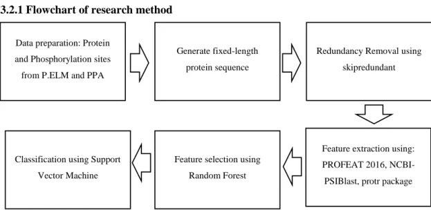
3.2.1 Flowchart of research method
Figure 3.1 Flowchart of the research method
We conducted six processes in our research, as shown in Figure 3.1 3.2.2 Feature extraction
Feature extraction generates a series of features by analyzing the original data. Using a fixed- length protein sequence, we implemented feature extraction to generate information as numerical vectors. The features that we used in this research were extracted using three tools: PROFEAT 2016 [10], NCBI-Psiblast [11], and protr package [12].
We extracted these features in this research: Amino Acid Composition (AAC), Dipeptide Composition (DPC), Normalized Moreau-Broto Autocorrelation Descriptors (NMB), Moran Autocorrelation Descriptors (MORAN), Geary Autocorrelation Descriptors (GEARY), Composition, Transition, Distribution (CTD), Sequence-Order-Coupling Number (SOCN), Quasi-Sequence-Order Descriptors (QSO),Amphiphilic Pseudo-Amino Acid Composition (APAAC), Total Amino Acid Properties (AAP), Position Specific Scoring Matrix (PSSM), BLOSUM and PAM Matrices for the 20 Amino Acid (BLOSUM), Amino Acid Properties Based Scales Descriptors (Protein Fingerprint) (ProtFP), Scales-based Descriptor derived by Principal Components Analysis (SCALES), Scales- based Descriptor derived by Multidimensional Scaling (MDDSCALES), and Conjoint Triad Descriptors (CTriad)
3.2.3 Protein feature selection using Random Forest
We implemented Random Forest for feature selection. We listed the important features based on the Gini Impurity index.
3.2.4 Support Vector Machine for phosphorylation site prediction
To classify whether a residue is phosphorylated, we used Support Vector Machine.
3.2.5 Evaluation Evaluation metrics
Data preparation: Protein and Phosphorylation sites from P.ELM and PPA
Generate fixed-length protein sequence
Redundancy Removal using skipredundant
Feature extraction using:
PROFEAT 2016, NCBI- PSIBlast, protr package Feature selection using
Random Forest Classification using Support
Vector Machine
5
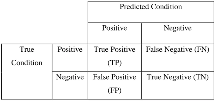
We conducted an evaluation to measure and compare the performance of classification results. Table 3.3 shows the combination of results of prediction compared to the results of real observations. True positive (TP) and True Negative (TN) occur when the result of the prediction is the same as the outcome of the real observation. False Positive (FP) and False Negative (FN) occur when the result of the prediction is different from the outcome of real observation.
Table 3.3 Combination of prediction outcomes with observation matrix
Predicted Condition Positive Negative True
Condition
Positive True Positive (TP)
False Negative (FN)
Negative False Positive (FP)
True Negative (TN)
Using the result of the classification which are True Positive (TP), False Negative (FN), False Positive (FP), True Negative (TN), we calculated this metrics
𝐴𝑐𝑐𝑢𝑟𝑎𝑐𝑦 =
𝑇𝑃+𝑇𝑁𝑇𝑃+𝑇𝑁+𝐹𝑃+𝐹𝑁
𝑆𝑒𝑛𝑠𝑖𝑡𝑖𝑣𝑖𝑦 =
𝑇𝑃𝑇𝑃+𝐹𝑁
𝑆𝑝𝑒𝑐𝑖𝑓𝑖𝑐𝑖𝑡𝑦 =
𝑇𝑁𝑇𝑁+𝐹𝑃
𝐹1 𝑠𝑐𝑜𝑟𝑒 = 2 ×
𝑇𝑃𝑇𝑃+𝐹𝑃+𝐹𝑁
Matthews Correlation Coefficient (MCC) 𝑀𝐶𝐶 =
(𝑇𝑃×𝑇𝑁)−(𝐹𝑃×𝐹𝑁)√(𝑇𝑃+𝐹𝑃)×(𝑇𝑃+𝐹𝑁)×(𝑇𝑁+𝐹𝑃)×(𝑇𝑁+𝐹𝑁)
Receiver Operating Character (ROC) Curve. An ROC curve is a commonly used way to visualize and evaluate the performance of a binary classifier. ROC compares the values of True Positive Rate with the False Positive Rate.
3.2.6 Grid search
Grid search is a method of finding the best number of features that achieve the highest accuracy
for classification. This method consist of two phases. In the first phase, we defined the class label
and the features. Then we split the data set into two sets, a data for training and a data for testing, by
using k–fold cross validation. Using the training data, we created a model with Random Forest and
listed the important features. We then set the grid length (for example, grid length=20), selected the
number of features, and added numbers of features based on grid length. Using the selected number
6
of features, we conducted cross validation for each number of feature selection. We selected the best number of features (X) that produced the highest accuracy from cross validation
In phase two, we conducted a finer grid search than phase one. The feature numbers that were selected were based on the numbers within the grid length of X. By selecting those feature numbers, we conducted cross validation. We then selected the number of the feature that had the highest accuracy (Y). Using the important list, we then selected Y number of features for the test and training data. We then generated a new model from the selected features in the training data and tested the model using the test data set, in which we also selected Y number of features. We conducted grid search for each fold. In addition, we recorded the result of the prediction.
4. Result and discussion
4.1 P.ELM data set
4.1.1 Important features
We conducted classification using the P.ELM data set. To evaluate the performance, we used ten times 10-fold cross validation. For each fold in each iteration, the model generates a list of important features measured. We averaged the value of each feature in the 100 lists and conducted a detailed analysis to determine which features were dominant and most influenced the classification method. An important features comparison was conducted for the P.ELM data set. We listed the top 20 important features for each residue, as shown in Table 4.1 List of top 20 important features in the P.ELM data set for Serine, Threonine, and Tyrosine residues.
Table 4.1 List of top 20 important features in the P.ELM data set for Serine, Threonine, and Tyrosine residues Rank Serine Threonine Tyrosine Rank
(cont’d)
Serine Threonine Tyrosine
1 QSO QSO QSO 11 CTD CTD CTD
2 AAC QSO QSO 12 CTD CTD CTD
3 QSO APAAC APAAC 13 DPC CTD CTD
4 APAAC AAC AAC 14 CTD CTD CTD
5 PSSM PSSM PSSM 15 CTD CTD CTD
6 CTD BLOSUM BLOSUM 16 CTD CTD CTD
7 CTD DPC DPC 17 CTD MDSSCALES MDSSCALES
8 CTD CTD CTD 18 CTD PROTFP PROTFP
9 CTD PSSM PSSM 19 PSSM PSSM PSSM
10 CTD SCALES SCALES 20 PSSM PSSM PSSM
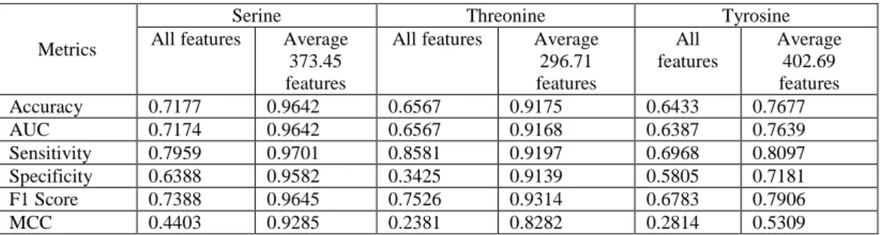
4.1.2 Classification result
By implementing feature selection with grid search for finding the best set of features,
performances were greatly improved, as shown in Table 4.2. For instance, Serine increased its
accuracy and had the highest accuracy at 96.46% using 373.45 important features in average (i.e. the
average number of features selected in 10 times 10-fold cross validation). This is followed by
Threonine at 91.75% using its averaged 296.71 important features. Tyrosine achieved its best
performance, 76.77%, using its averaged 402.69 important features. Based on the comparison of
7
before and after using feature selection, Threonine had the largest percentage of increase in accuracy, 26.08%, followed by Serine, 24.68%, and Tyrosine, 12.44%.
Since feature selection decreased the performance in Ismail’s work, it is an important finding that under an appropriate combination of classifier and features, feature selection could improve the performance of protein phosphorylation site prediction.
Table 4.2 Performance of classification using all of the features (2292 features) and best result of features selection for P.ELM data set
Metrics
Serine Threonine Tyrosine
All features Average 373.45 features
All features Average 296.71 features
All features
Average 402.69 features
Accuracy 0.7177 0.9642 0.6567 0.9175 0.6433 0.7677
AUC 0.7174 0.9642 0.6567 0.9168 0.6387 0.7639
Sensitivity 0.7959 0.9701 0.8581 0.9197 0.6968 0.8097
Specificity 0.6388 0.9582 0.3425 0.9139 0.5805 0.7181
F1 Score 0.7388 0.9645 0.7526 0.9314 0.6783 0.7906
MCC 0.4403 0.9285 0.2381 0.8282 0.2814 0.5309
4.2 PPA data set
4.2.1 Important features
For the PPA data set, we also conducted classification. We evaluated performance using Leave-One-Out cross validation. Based on each fold, using Random Forest, an important feature list was generated from the training data. Therefore, the number of important feature lists generated equals the number of observations in the data set. As in the P.ELM data set, we measured the average value of each feature in all the feature lists.
Important feature comparison is also conducted for the PPA data set. We list top 20 important feature for each residue as shown in Table 4.3.
Table 4.3 List of top 20 important features in the PPA data set for Serine, Threonine, and Tyrosine residues Rank Serine Threonine Tyrosine Rank
(cont’d)
Serine Threonine Tyrosine
1 QSO APAAC QSO 11 CTD CTD QSO
2 QSO QSO AAP 12 CTD CTD CTD
3 APAAC QSO SOCN 13 AAP MDSSCALES QSO
4 AAC AAC QSO 14 CTD MDSSCALES PSSM
5 CTD CTD CTD 15 CTD MDSSCALES QSO
6 CTD CTD QSO 16 CTD MDSSCALES BLOSUM
7 CTD APAAC CTD 17 CTD BLOSUM MDSSCALES
8 CTD QSO APAAC 18 CTD MDSSCALES SCALES
9 CTD QSO CTD 19 CTD SCALES APAAC
10 CTD AAC AAP 20 CTD MDSSCALES QSO
4.2.2 Classification result
In general, as shown in Table 4.4, we can see that without feature selection the accuracy is
lower than 70% for all three data sets. However, there is an improvement if we implement feature
selection before conducting class prediction. Threonine has the highest accuracy, 86.76%, using the
8
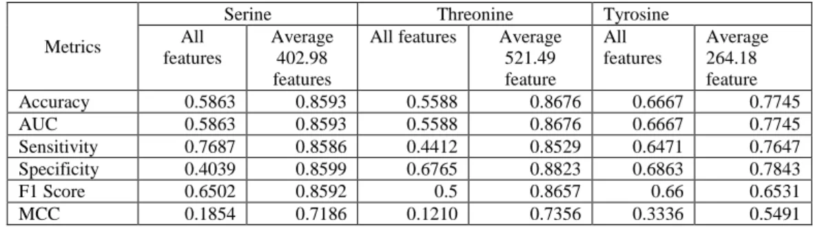
averaged 521.49 important features. This is followed by Serine, achieving 84.73% accuracy using the averaged 403.98 important features. Tyrosine has the lowest accuracy, achieving 77.45% using the averaged 264.18 important features.
If we compare the increase in performance between not using feature selection and feature selection, Threonine achieved a 30.88% increase in accuracy, followed by Serine’s 27.30% increase.
Tyrosine has the lowest increase of accuracy at 10.78%.
Table 4.4 Performance of classification using all of the features (2292 features) and best result of features selection for PPA data set
Metrics
Serine Threonine Tyrosine
All features
Average 402.98 features
All features Average 521.49 feature
All features
Average 264.18 feature
Accuracy 0.5863 0.8593 0.5588 0.8676 0.6667 0.7745
AUC 0.5863 0.8593 0.5588 0.8676 0.6667 0.7745
Sensitivity 0.7687 0.8586 0.4412 0.8529 0.6471 0.7647
Specificity 0.4039 0.8599 0.6765 0.8823 0.6863 0.7843
F1 Score 0.6502 0.8592 0.5 0.8657 0.66 0.6531
MCC 0.1854 0.7186 0.1210 0.7356 0.3336 0.5491
4.3 Comparison with other previous data set
In this research, we compared the result from our method to several other previous research works on phosphorylation site prediction. The compared methods are as follows: Netphos [13] , NetphosK [1], GPS 2.1 [2], Swaminathan, PPRED [14], Musite [15], PhosphoSVM [3], and RF-Phos [4]. Most of the previous research did not conduct feature selection to improve the classification of phosphorylation sites. Only RF-Phos implemented feature selection using Random Forest.
4.3.1 Classification result P.ELM Data Set
In this work, we also compared the result from the P.ELM data set and the PPA data set with other results from previous research. Table 4.5 shows the performance comparison between our results and other results. For Serine and Threonine, our method achieved the highest AUC, sensitivity, and MCC values. However, our specificity value from the Threonine data set is lower than the result of RF-Phos. On the other hand, in the Tyrosine data set our method achieved a lower AUC, specificity, and MCC, in comparison with the result of RF-Phos.
Table 4.5 Performance comparison of several phosphorylation site prediction methods for Serine, Threonine, and Tyrosine residues using the P.ELM data set
Methods
Serine Threonine Tyrosine
AUC Sen Spec MCC AUC Sen Spec MCC AU
C
Sen Spec MCC NetPhosK 0.63 0.509 0.678 0.08 0.60 0.620 0.568 0.07 0.60 0.395 0.742 0.08 GPS 2.1 0.73 0.331 0.933 0.20 0.70 0.381 0.923 0.20 0.61 0.345 0.789 0.08 Swaminathan 0.70 0.313 0.887 0.13 0.72 0.280 0.925 0.14 0.62 0.605 0.570 0.09 NetPhos 0.70 0.341 0.867 0.12 0.66 0.343 0.837 0.09 0.65 0.347 0.845 0.13 PPRED 0.75 0.323 0.916 0.17 0.73 0.303 0.910 0.13 0.70 0.430 0.827 0.17
9
Musite 0.81 0.414 0.937 0.25 0.78 0.338 0.948 0.22 0.72 0.384 0.867 0.18 PhosphoSVM 0.84 0.444 0.940 0.30 0.82 0.378 0.950 0.25 0.74 0.419 0.873 0.21 RF-Phos 0.88 0.840 0.850 0.65 0.90 0.830 0.940 0.70 0.91 0.830 0.880 0.70 Our Method 0.96 0.970 0.958 0.93 0.92 0.920 0.914 0.83 0.77 0.810 0.759 0.53
PPA Data Set
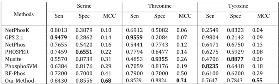
We also compared our classification results with the results in other research. The methods we compared are: NetphosK, GPS 2.1, NetPhos, PHOSPHER, Musite, PhosphoSVM, and RF-Phos. In Table 4.6, we can see that our method has a lower performance in sensitivity and specificity, for all residues. However, achieving the best MCC for all residues is of higher importance.
Table 4.6 Performance comparison of several phosphorylation site prediction methods for Serine, Threonine, and Tyrosine residues using the PPA data set
Methods
Serine Threonine Tyrosine
Sen Spec MCC Sen Spec MCC Sen Spec MCC
NetPhosK 0.8013 0.3879 0.10 0.6912 0.5082 0.06 0.2549 0.8323 0.04 GPS 2.1 0.9479 0.2862 0.14 0.9559 0.2084 0.07 0.9804 0.2142 0.09 NetPhos 0.7655 0.5420 0.16 0.5441 0.7743 0.12 0.6471 0.6750 0.13 PHOSFER 0.7459 0.6551 0.22 0.7794 0.6477 0.14 0.6275 0.5929 0.08 Musite 0.5570 0.8739 0.31 0.4853 0.9355 0.26 0.4706 0.8877 0.20 PhosphoSVM 0.6384 0.8176 0.29 0.7059 0.8176 0.19 0.8235 0.6418 0.18 RF-Phos 0.7200 0.7000 0.41 0.7900 0.7000 0.50 0.6100 0.6200 0.29 Our Method 0.8430 0.8556 0.68 0.8529 0.8824 0.74 0.7647 0.7843 0.55
4.3.2 Feature selection
Table 4.7 shows a comparison of the top ten important features used in our method and RF-Phos.
Both of these lists are used to classify phosphorylation sites using the P.ELM data set.
Table 4.7 Comparison of the top 10 important features between RF-Phos and our method for phosphorylation site prediction using the P.ELM data set
Rank RF-Phos Our Method
Serine Threonine Tyrosine Serine Threonine Tyrosine
1 QSO QSO CTD QSO QSO QSO
2 OP QSO CTD AAC QSO QSO
3 QSO SF ASA QSO APAAC APAAC
4 SF OP IG APAAC AAC AAC
5 CTD CTD OP PSSM PSSM PSSM
6 ACH CTD CTD CTD BLOSUM BLOSUM
7 ACH CTD CTD CTD DPC DPC
8 ASA OP CTD CTD CTD CTD
9 CTD CTD CTD CTD PSSM PSSM
10 ASA CTD ASA CTD SCALES SCALES