Adaptive Output Feedback Control of General MIMO Systems Using Multirate Sampling
Ikuro Mizumoto* Satoshi Ohdaira Makoto Kumon Zenta Iwai Department of Mechanical Engineering
and Materials Science Kumamoto University
2-39-1 Kurokami, Kumamoto, 860-8555, Japan
*
[email protected]Tongwen Chen
Department of Electrical and Computer Engineering
University of Alberta
Edmonton, Alberta, Canada T6G 2V4
Abstract— In adaptive output feedback control based on
almost strictly positive real conditions, a technical difficulty arises when the multi-input multi-output (MIMO) system under consideration is non-square, and in particular, has less inputs than outputs. To overcome this, we propose an idea of multirate sampled-data control. That is, a lifted discrete-time system, which has the same number of inputs and outputs and does not give rise to the causality constraint, is made by carefully choosing faster input sampling rates. The output feedback based adaptive control strategy can then be applied to the lifted system under certain conditions. The results reported here are validated on numerical simulations through a cart-crane model.
I. I
NTRODUCTIONMultirate systems arise often in industry due to hardware limitations on sensoring and actuating devices. In such in- herently multirate sampled systems, one is forced to consider multirate control strategies such as multirate robust control [5], and multirate adaptive control [13], [17], [6], which are more relevant to the topic in this paper.
However, the multirate systems in this paper are motivated from a different viewpoint. In adaptive output feedback control design based on almost strictly positive real (ASPR) conditions, under certain assumptions, closed-loop stability can be proven for single-input, single-output plants and robustness of the adaptive scheme has been shown [9], [7], [12]. Such an adaptive control scheme has several practical advantages and has been applied successfully to many industrial applications. Extending this scheme to multi- input, multi-output systems, the design procedure requires a technical assumption that the systems to be controlled must be square, i.e., the number of inputs must be equal to the number of outputs [3], [1], [8], [15]. Such an assumption can be quite restrictive – in many practical systems, the number of inputs is less than that of the outputs, especially in cases where several control objectives are to be achieved. In such cases, how to apply the adaptive control design methodology is the thrust of this research. Our idea is to consider digital control with a multirate sampling scheme. Thus multirate systems in this paper are obtained by control designers on purpose in order to accommodate existing adaptive control strategies.
In selecting the different sampling rates involved, there are two points that we need to keep in mind:
•
First, we need to ensure that the resultant systems after lifting [11], [10] are square (with the same number of inputs and outputs).
•
Second, we need to avoid further complication by introducing another difficult design limitation – the so called causality constraint, see, e.g., [5].
We will show later that these two goals can be achieved simultaneously by carefully choosing faster input updating rates only.
II. M
ULTIRATES
AMPLING ANDL
IFTINGFor a general discussion, consider a continuous-time, linear, time-invariant plant G
cwith m inputs and p outputs, and p > m; assume a state-space representation for G
cwith input u
c, output y
c, and state x
c:
˙
x
c(t) = A
cx
c(t) + B
cu
c(t), (1) y
c( t ) = Cx
c( t ) + D
cu
c( t ) . (2) Partitioning B
cand D
caccording to the input u
c, we get B
cD
c=
B
c1B
c2· · · B
cmD
c1D
c2· · · D
cm, u
c=
⎡
⎢ ⎢
⎢ ⎣ u
c1u
c2.. . u
cm⎤
⎥ ⎥
⎥ ⎦ ,
in which B
c1, B
c2, · · · , B
cmare n-dimensional column vec- tors, with n being the dimension of the state space, and D
c1, D
c2, · · · , D
cmare m-dimensional column vectors.
The system G
cis a typical non-square system; now we would like to derive a square lifted discrete-time system.
There are many different ways to arrive at a square lifted system by selecting multiple sampling rates, but we target simple ones which do not introduce the causality constraint later in the design of the controller.
We choose to sample all outputs uniformly with a single period, say, T , and update the inputs u
c1, u
c2, · · · , u
cmthrough zero-order holds with fast periods T /q
1, T /q
2,
· · ·, T /q
m, respectively. Here q
1, q
2, · · · , q
mare all positive integers and are chosen to satisfy
q
1+ q
2+ · · · + q
m= p. (3)
Proceedings of the
44th IEEE Conference on Decision and Control, and the European Control Conference 2005
Seville, Spain, December 12-15, 2005
WeA10.2
- Hmr - G
c- S
T-
u u
cy
cy
Fig. 1. The multirate sampled-data system
We remark that such q
i’s always exist (if m < p) and are non-unique; e.g., if m = 2 and p = 5, there are four possible (q
1, q
2) pairs satisfying (3); they are (1, 4), (2, 3), (3, 2), and (4, 1).
Denote the correspondingly discretized system by G; this is a multirate discrete-time system depicted in Figure 1, where S
Tis an ideal sampler with period T (vector-valued), and Hmr is the multirate zero-order hold operator defined as
Hmr =
⎡
⎢ ⎢
⎢ ⎣ H
T/q1H
T/q2. ..
H
T/qm⎤
⎥ ⎥
⎥ ⎦
with H
T/qibeing the synchronized zero-order hold with period T /q
i. Note that y is single-rate with period T (y = S
Ty
c), but u is multirate with each component having a different period; we can write
u =
⎡
⎢ ⎣ u
1.. . u
m⎤
⎥ ⎦ , u
ci= H
T/qiu
i, i = 1, 2, · · · , m.
We get that the multirate G takes multirate u into single-rate y, and can be denoted by
G = S
TG
cHmr .
Next, we need to lift this multirate system to arrive at a time-invariant one with the single period T .
Let v be a discrete-time signal defined on the time set {0 , 1 , 2 , · · ·} :
v = {v(0), v(1), v(2), · · ·}.
The q-fold lifting operator L
qmaps v into v as follows [11], [10]:
v =
⎧ ⎪
⎪ ⎪
⎨
⎪ ⎪
⎪ ⎩
⎡
⎢ ⎢
⎢ ⎣ v (0) v (1) .. . v ( q − 1)
⎤
⎥ ⎥
⎥ ⎦ ,
⎡
⎢ ⎢
⎢ ⎣
v ( q ) v ( q + 1)
.. . v (2 q − 1)
⎤
⎥ ⎥
⎥ ⎦ , · · · ,
⎫ ⎪
⎪ ⎪
⎬
⎪ ⎪
⎪ ⎭ .
Notice that the lifting operation increases the dimension of the signal by a factor of q, but decreases the underlying sampling rate also by a factor of q. The inverse lifting operation, L
−1qis defined obviously.
In order to get a lifted system which is single-rate with period T , we lift the input u
iby L
qito get u
iso that the lifted system G maps u(k) into y(k) defined as follows:
u ( k ) =
⎡
⎢ ⎣ u
1( k )
.. . u
m( k )
⎤
⎥ ⎦ .
Thus we can write
G = G
⎡
⎢ ⎣ L
−1q1. ..
L
−1qm⎤
⎥ ⎦
This G is square and m × m, based on (3). It is a fact that G is time-invariant and admits a state-space model, which can be derived based on the results in [5], [4]. We summarize the results into a few steps.
Step 1 Compute the step-invariant transformation ma- trices as follows:
A = e
AcT,
A
i= e
AcT/qi, B
i=
T/qi0
e
ActB
cidt, i = 1, 2, · · · , m.
Step 2 Define the matrices B
i=
A
qii−1B
i· · · A
iB
iB
i, D
i=
D
ci0 · · · 0
, i = 1, 2, · · · , m.
Step 3 Then a state-space model for G is given by x ( k + 1) = Ax ( k ) + Bu ( k ) , (4)
y(k) = Cx(k) + Du(k), (5) where x(k) = x
c(kT ), and
B =
B
1B
2· · · B
m,
D =
D
1D
2· · · D
m.
Because of the choice of sampling rates, the causality con- straint in the lifted controller (mapping y into u) will not arise [5].
III. A
DAPTIVEC
ONTROLD
ESIGNThe adaptive controller design is based on the lifted system G in (4) and (5); such controllers map y into u. Hence in implementation to the original sampled-data system, the controller output u needs to be inverse-lifted properly.
A. Problem Statement
Consider the lifted, but square system G in (4) and (5);
we shall need a few conditions in order to proceed.
Definition 1: (Almost Strictly Positive Realness [1], [9]) The square plant G in (4) and (5) is called almost strictly positive real (ASPR) if there exists a static output feedback such that the resulting closed loop system is strictly positive real (SPR). Explicitly, G is ASPR if there exists a control input with a feedback gain Θ
∗,
u(k) = −Θ
∗y(k) + v(k), (6) (v is any external input) such that the resulting closed loop system from v(k) to y(k),
x ( k + 1) = A
cx ( k ) + B
cv ( k ) , (7)
y(k) = C
cx(k) + D
cv(k), (8)
with
A
c= A − B Θ
∗( I + D Θ
∗)
−1C , B
c= B ( I + Θ
∗D )
−1, C
c= ( I + D Θ
∗)
−1C , D
c= D ( I + Θ
∗D )
−1,
(9) is SPR.
Definition 2: The square plant G is called strongly ASPR if there exists a static output feedback,
u(k) = −Θ
∗y(k) + v(k),
such that the closed loop system with state matrices (A
c, B
c, C
c, D
c) as given in (9) is SPR and, in addition, a transformed closed loop system with v ˜ = (I + Θ
∗D)
−1v as input,
x(k + 1) = A
cx(k) + B v(k) ˜ (10) y(k) = C
cx(k) + D v(k) ˜ (11) is also SPR.
The sufficient conditions for G to be ASPR are easily obtained by translating the conditions given for continuous- time systems [2] as follows.
ASPR Conditions:
(1) The relative MacMillan degree of the system is n/n, where n is the dimension of the A-matrix.
(2) The plant is minimum-phase.
Furthermore, for strong almost strictly positive realness, an additional condition is required:
(3) D + D
T> 0.
We shall impose the following assumptions on the lifted model G in (4) and (5).
Assumption 1: The plant G given in (4) and (5) is con- trollable and observable.
This assumption can be related to controllability and observability of the original continuous-time system and a non-pathological sampling condition [4], [5].
Assumption 2: The direct feedthrough matrix D in (5) is known.
Assumption 3: For the plant G given in (4) and (5), there exists a known stable parallel feedforward compensator (PFC), denoted by G
f, with a state-space model of an appropriate order,
x
f(k + 1) = A
fx
f(k) + B
fu(k), (12) y
f( k ) = C
fx
f( k ) + D
fu ( k ) , (13) such that the resulting augmented system, G + G
f, with a state-space model,
x
a(k + 1) = A
ax
a(k) + B
au(k), (14) y
a( k ) = C
ax
a( k ) + D
au ( k ) , (15) is strongly ASPR. Here, x
a( k ) = [ x ( k )
Tx
f( k )
T]
Tand A
a=
A 0 0 A
f, B
a=
B B
f, C
a=[ C C
f] , D
a= D + D
f.
It should be noted that under Assumption 3, there exists a static output feedback with a feedback gain matrix Θ ˜
∗e> 0,
u ( k ) = − ˜Θ
∗ey
a( k ) + v ( k )
such that the resulting closed loop system, after an input transformation v ˜ = (I + ˜Θ
∗eD
a)
−1v,
x
a(k + 1) = A
acx
a(k) + B
av(k), ˜ y
a( k ) = C
acx
a( k ) + D
a˜ v ( k ) , is SPR. In this case,
A
ac= A
a− B
a˜Θ
∗e(I + D
a˜Θ
∗e)
−1C
a, C
ac= (I + D
a˜Θ
∗e)
−1C
a.
Further, since the system ( A
ac, B
a, C
ac, D
a) is SPR, there exist positive symmetric matrices P = P
T> 0 , Q = Q
T>
0 and appropriate matrices L and W such that based on the Kalman-Yakubovich Lemma, the following hold:
A
TacP A
ac− P = −LL
T− Q, A
TacP B
a= C
acT− LW
T,
B
aTP B
a= D
a+ D
aT− W W
T.
(16) Our control objective in this paper is to design an adaptive controller that achieves
k→∞
lim y(k) = 0, (17) for G satisfying Assumptions 1 to 3.
B. Controller Design Procedure
An adaptive controller for attaining the control objective in (17) can be designed by the following equations [ 12 ] , [ 15 ] : u(k) = −Θ
e(k)y
p(k), (18) y
p( k ) = C
ax
a( k ) . (19) The feedback gain matrix Θ
e(k) in (18) is adaptively ad- justed by the following parameter adjusting law:
Θ
e(k) = Θ
P e(k) + Θ
Ie(k), (20) Θ
P e( k ) = y
a( k ) y
pT( k )Γ
P e, (21) Θ
Ie(k) = Θ
Ie(k − 1) + y
a(k)y
pT(k)Γ
Ie. (22) Here Γ
P e= Γ
TP e> 0, Γ
Ie= Γ
TIe> 0.
It is noted that y
a(k) in (21) and (22) cannot be directly obtained from measured signals because of a causality prob- lem which arises from the direct feedthrough term D
ain (15). However, y
a( k ) can be generated by using available signals. From (15) and (18), we have
y
a( k ) = y
p( k )+ D
au ( k )
= y
p(k)−D
a{Θ
Ie(k−1)+y
a(k)y
pT(k)Γ
e}y
p(k) (23) where Γ
e= Γ
P e+ Γ
Ie. Therefore y
a(k) can be obtained by
y
a(k) = {I + D
ay
pT(k)Γ
ey
p(k)}
−1×{y
p(k) − D
aΘ
Ie(k − 1)y
p(k)},
by using available signals.
C. Stability Analysis
We have the following stability result for the resulting closed loop control system.
Theorem 1: Under Assumptions 1 to 3, all the signals in the resulting closed loop control system with control input in (18) are uniformly bounded and the output converges to zero, i.e., the objective lim
k→∞y(k) = 0 is achieved.
Proof. Consider an ideal control input given by
u
∗( k ) = −Θ
∗ey
p( k ) , (24) Θ
∗e= (I + ˜Θ
∗eD
a)
−1˜Θ
∗e= ˜Θ
∗e(I + D
a˜Θ
∗e)
−1. (25) The closed loop system with control input in (18) can be represented by
x
a( k + 1) = ˜ A
ax
a( j ) + B
a∆ u ( k ) , (26) y
a(k) = ˜ C
ax
p(j) + D
a∆u(k), (27) where
A ˜
a= A
a− B
aΘ
∗eC
a(28) C ˜
a= (I − D
aΘ
∗e)C
a(29)
∆ u ( k ) = u ( k ) − u
∗( k )
Now, consider the following positive definite function V ( k ) ,
V (k) = V
1(k) + V
2(k), (30) V
1( k ) = x
a( k )
TP x
a( k ) , (31) V
2(k) = tr{∆Θ
Ie(k − 1)Γ
−1Ie∆Θ
TIe(k − 1)}, (32) where
∆Θ
Ie( k ) = Θ
Ie( k ) − Θ
∗e. (33) Defining ∆ V ( k ) by
∆ V ( k ) = V ( k + 1) − V ( k ) , (34) we have from (30) that
∆V (k) = ∆V
1(k) + ∆V
2(k) (35)
∆ V
1( k ) = V
1( k + 1) − V
1( k )
∆V
2(k) = V
2(k + 1) − V
2(k)
First, consider the difference ∆ V
1. We have from (26) and (31) that
∆ V
1( k ) = V
1( k + 1) − V
1( k )
= x
a(k)
T{ A ˜
TaP A ˜
a− P }x
a(k) +2x
a(k)
TA ˜
TaP B
a∆u(k)
+∆ u ( k )
TB
aTP B
a∆ u ( k ) . (36) Since it follows from (25) that
I − D
aΘ
∗e= I − D
a˜Θ
∗e( I + D
a˜Θ
∗e)
−1= (I + D
a˜Θ
∗e)
−1= 0 (37) we have from (28), (29) and (25) that
A ˜
a= A
a− B
a˜Θ
∗e( I + D
a˜Θ
∗e)
−1C
a= A
ac, (38) C ˜
a= (I + D
a˜Θ
∗e)
−1C
a= C
ac, (39)
Thus, since the system ( A
ac, B
a, C
ac, D
a) is SPR, ∆ V
1( k ) can be expressed from (16) and (36) as
∆ V
1( k ) = − x
a( k )
TQx
a( k ) + 2 y
a( k )
T∆ u ( k )
−x
a(k)
TL − ∆u(k)
TW
2(40) Next, consider the difference ∆ V
2. From (22) and (33), we have
∆Θ
Ie( k ) = ∆Θ
Ie( k − 1) − y
a( k ) y
p( k )
TΓ
Ie(41) Thus ∆V
2(k) can be expressed as
∆V
2(k) = 2tr{∆Θ
Ie(k)y
p(k)y
a(k)
T}
− tr { y
a( k ) y
p( k )
TΓ
Iey
p( k ) y
a( k )
T} . Since
∆Θ
Ie( k ) = ∆Θ
e( k ) − y
a( k ) y
p( k )
TΓ
P e, (42)
∆Θ
e(k) = Θ
e(k) − Θ
∗e, it follows that
∆ V
2( k ) = −2 y
a( k )
T∆ u ( k )
−tr{y
a(k)y
p(k)
T(Γ
Ie+ 2Γ
P e)y
p(k)y
a(k)
T}.
(43) Finally, from (40) and (43) , ∆ V ( k ) can be evaluated as follows:
∆ V ( k ) = − x
a( k )
TQx
a( k ) − x
a( k )
TL − ∆ u ( k )
TW
2−tr{y
a(k)y
p(k)
T(Γ
Ie+ 2Γ
P e)y
a(k)y
a(k)
T}
≤ 0. (44)
Consequently we have that x
a( k ) and Θ
Ie( k ) are uniformly bounded and then it is easy to conclude that all the signals in the control system are uniformly bounded. Further, since we have from (44) that
N→∞
lim
N k=0x
a( k )
2< ∞ ,
we can obtain lim
k→∞x
a( k ) = 0 and thus we have lim
k→∞x(k) = 0. Moreover, from (18) and (19) we have lim
k→∞y
p(k) = 0 and lim
k→∞u(k) = 0. Therefore, we can conclude from (5) that
k→∞
lim y(k) = 0.
Remark: In practical applications in which disturbances and
measurement noises exist, one cannot guarantee the stability
of the resulting control system with the ideal adaptive
parameter adjusting law (22). However, in such cases, one
can adopt robust adaptive parameter adjusting laws such as
the one with σ-modification [1], [7] in order to guarantee
boundedness of all signals in the control system.
y M
I m, u
L
φ c1
c2
g
Fig. 2. Cart-crane system
Table 1 Parameters of cart-crane system
Parameter Value
g 9.81 [m/s
2] M 1.168 + 3 [kg]
m 0.071 [kg]
L 0.358 [m]
I 3 . 025 × 10
−3[ kg · m
2] c
10.01 [N·s/rad]
c
210 [ N · s/m ] IV. N
UMERICALS
IMULATIONIn this section, we validate the effectiveness of the pro- posed method through numerical simulations for a cart-crane model. A simple configuration of the cart-crane system is illustrated in Fig. 2, in which φ(t) is the angular position of the crane, y(t) is the displacement of the cart, and u(t) is the control force applied to the cart; the system parameters involved are M (mass of the cart), m (mass of the crane), L (length from the axis of rotation to the center of gravity of the crane), I (moment of inertia of the crane), g (gravitational acceleration), c
1(damping constant at the rotational axis), and c
2(damping constant between the cart and the horizontal surface). These parameters are given in Table 1 above.
Define x
c(t) = [φ(t), φ(t), y(t), ˙ y(t)] ˙
T, y
c(t) = [ φ ( t ) , y ( t )], and u
c= u. A linearized state-space model around φ = 0 for the cart-crane system is given as follows:
˙
x
c(t) =
⎡
⎢ ⎢
⎣
0 1 0 0 a b 0 c 0 0 0 1 d e 0 f
⎤
⎥ ⎥
⎦ x
c(t) +
⎡
⎢ ⎢
⎣ 0 g
10 h
⎤
⎥ ⎥
⎦ u
c(t) (45)
y
c( t ) =
1 0 0 0 0 0 1 0
x
c( t ) (46) with
a = (m − M )mgL
∆ , b = (m − M )c
1L
∆ , c = −mLc
2∆ d = m
2gL
2∆ , e = mL
2c
1∆ , f = − mL
2c
2− Ic
2∆ g
1= mL
∆ , h = mL
2+ I
∆ , ∆ = mM L
2+ I ( M − m ) . In this simulation, we assume that the output y
c(t) is sampled with a period of T = 0.2 [s], but the input signal u
c(t) can be updated through a zero-order hold with a fast period T /2. Furthermore, to improve the control performance
0 5 10 15 20
−0.5
−0.4
−0.3
−0.2
−0.1 0 0.1 0.2
time [sec]
outputs
angle [rad]
position [m]
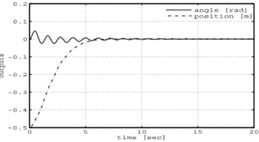
Fig. 3. Simulation result with multirate adaptive controller: cart position and crane angle
0 5 10 15 20
−6
−4
−2 0 2 4 6
time [sec]
input
force [N]
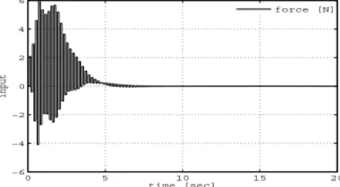
Fig. 4. Simulation result with multirate adaptive controller: control input
for the crane angle, we consider a weighted angle, that is, we generate
y
cw(t) =
w
10 0 1
y
c(t) (47) as a new output for the controller design. In this simulation, we set w
1= 20. A PFC, which renders the resulting augmented system ASPR, is designed as follows:
D
p=
0 . 02 0 0 0 . 02
for the system with y
cwas the output. This is the case where A
f= 0, B
f= 0, C
f= 0, and D
f= D
pis the PFC in (12) and (13). Parameters in the adaptive adjusting laws in (20) to (22) are set to
Γ
P e= diag [10 , 10] , Γ
Ie= diag [8 , 8] .
Figs. 3 and 4 show simulation results of the proposed multirate control strategy – vibration of the pendulum is effectively suppressed and the cart moves smoothly to the desired position.
By way of comparison, we apply a PI controller to this cart-crane system under the assumption that all the outputs can be sampled with as fast as the control updating period T = 0 . 1 [s]. The (digital) PI controller is then designed as follows:
u
P I( k ) = −
K
Py ˆ
P I( k ) + T K
I k m=0ˆ y
P I( m )
(48) ˆ
y
P I(k) = w
p1φ(k) + w
p2y(k). (49) Here K
pand K
Iare the proportional and integral gains of the PI controller; w
p1and w
p2are weighting factors for the outputs φ(t) and y(t).
The PI controller parameters are designed to obtain a good cart positional control, and are given as follows:
K
P= 23, K
I= 0.01, w
p1= 1, w
p2= 0.2.
0 5 10 15 20
−0.5
−0.4
−0.3
−0.2
−0.1 0 0.1 0.2
time [sec]
outputs
angle [rad]
position [m]
Fig. 5. Simulation result with PI controller for case-1: cart position and crane angle
0 5 10 15 20
−0.5 0 0.5 1 1.5 2 2.5
time [sec]
input
force [N]
Fig. 6. Simulation result with PI controller for case-1: control input
Figs. 5 and 6 show simulation results with this PI controller, which show a good control performance for the cart position, however, a crane angle vibration exists to some extent.
Comparing the results of the two control strategies, we conclude that the proposed multirate adaptive control is better in that good control performance for both cart position and crane angle is achieved simultaneously.
Next, in order to test the adaptive strategy, we consider a situation in which a load is attached to the tip of the crane, and thus both the weight and center of gravity of the crane are changed. In the simulation we take the load to be 50m. Fig. 7 shows the result with the PI controller;
the control performance is poor and the control system is even unstable. On the other hand, the control result (Fig.
8) with the proposed multirate adaptive controller shows approximately the same performance as in Fig. 3 with no load. Thus the proposed multiratre adaptive controller has a better robustness properties against parameter variations than the conventional PI controller.
V. C
ONCLUSIONSIn this paper, we proposed an adaptive output feedback design scheme for general MIMO systems using the idea of multirate sampled data control. The scheme was based on the ASPR-ness of a controlled system with a condition that the controlled system must be square (namely, with the same number of inputs and outputs). To satisfy this condition, a square lifted discrete-time system was created by using a multirate sampling technique. An ASPR based adaptive control scheme was then applied to this lifted system. The obtained adaptive controller is then multirate and can be implemented to non-square MIMO systems. The effectiveness of the proposed method was validated through numerical simulations for a cart-crane model.
0 5 10 15 20
−4
−3
−2
−1 0 1 2 3 4
time [sec]
outputs
angle [rad]
position [m]
Fig. 7. Simulation result with PI controller: additional load
0 5 10 15 20
−0.5
−0.4
−0.3
−0.2
−0.1 0 0.1 0.2
time [sec]
outputs
angle [rad]
position [m]
Fig. 8. Simulation result with multirate adaptive controller: additional load
R
EFERENCES[1] I. Bar-Kana, “Absolute stability and robust discrete adaptive control of multivariable systems,”Control and Dynamic Systems, vol. 31, pp.
157-183, 1989.
[2] I. Bar-Kana, “Positive realness in multivariable stationary linear sys- tems,”Journal of Franklin Institute, vol. 328, no. 4, pp. 403-417, 1991.
[3] I. Bar-Kana and H. Kaufman, “Global stability and performance of a simplified adaptive algorithm,”International Journal Control, vol. 42, no. 6, pp. 1491-1505, 1985.
[4] T. Chen and B.A. Francis,Optimal Sampled-data Control Systems, London: Springer, 1995.
[5] T. Chen and L. Qiu, “H∞design of general multirate sampled-data control systems,”Automatica, vol. 30, no. 7, pp. 1139-1152, 1994.
[6] M. Ishitobi, M. Kawanaka, and H. Nishi, “Ripple-suppressed multirate adaptive control,”15th World Congress of the International Federation of Automatic Control, Barcelona, Spain, 21-26 July 2002.
[7] Z. Iwai and I. Mizumoto, “Robust and simple adaptive control systems, International Journal of Control, vol. 55, no. 6, pp. 1453-1470, 1992.
[8] Z. Iwai and I. Mizumoto, “Realization of simple adaptive control by using parallel feedforward compensator,”International Journal of Control, vol. 59, no. 6, pp. 1543-1565, 1994.
[9] H. Kaufman, I. Bar-Kana and K. Sobel, Direct Adaptive Control Algorithms: Theory and Applications(2nd Ed.), Springer-Verlag, 1998.
[10] P.P. Khargonekar, K. Poolla, and A. Tannenbaum, “Robust control of linear time-invariant plants using periodic compensation,”IEEE Trans.
on Automatic Control, vol. 30, pp. 1088-1096, 1985.
[11] G.M. Kranc, “Input-output analysis of multirate feedback systems,”
IRE Trans. Automatic Control, vol. 3, pp. 21-28, 1957.
[12] H. Ohtsuka, I. Mizumoto, and Z. Iwai, “A discrete SAC system with parallel feedforward Compensators,”Trans. of Society of Instrument and Control Engineers, vol. 34, no. 2, pp. 96-104, 1998 (in Japanese).
[13] R. Scattolini, “Self-tuning control of systems with infrequent and delayed output sampling,”IEE Proceedings, Part D, Control Theory and Applications, vol. 135, no. 4, pp. 213-221, 1988.
[14] J. Sheng, T. Chen and S.L. Shah, “Generalized predictive control for non-uniformly sampled systems,”J. Process Control, vol. 12, no. 8, pp. 875-885, 2002.
[15] H. Shibata and T. Kurebayashi, “New discrete-time algorithm for simple adaptive control,”Trans. of Society of Instrument and Control Engineers, vol. 31, no. 2, pp. 177-184, 1995 (in Japanese).
[16] A.K. Tangirala, D. Li, R.S. Patwardhan, S.L. Shah and T. Chen,
“Ripple-free conditions for lifted multirate control systems,”Automat- ica, vol. 37, no. 10, pp. 1637-1645, 2001.
[17] C. Zhang, R.H. Middleton and R.J. Evans, “An algorithm for multirate sampling adaptive control,”IEEE Trans. Automatic Control, vol. 34, no. 7, pp. 792-795, 1989.