Using Moving Particle Semi-Implicit And Mass Spring System

Using Moving Particle Semi-Implicit And Mass Spring System

Mourice Woran

, Seiro Omata

a

Faculty of Mathematics and Natural Sciences, Institut Teknologi Bandung, Jl. Ganesha 10, Bandung 40132 Indonesia.

b

Institute of Science and Engineering, Kanazawa University, Kakuma, Kanazawa 920-1192 Japan, E-mail: moris [email protected]

Abstract. Interactions between fluids and deformable solid objects are very important in practical applications and it is an essential task to be able to simulate them correctly. A model for this kind of simulation is presented. The fluid is handled by use of a particle method, the so-called moving particle semi-implicit (MPS), whereas the solid is modeled by a spring-mass system which main- tains its volume throughout the simulation. The interaction relies on the coupling force between the solid and the fluid, through which the movements of both parts influence each other.

Keywords: Fluid-solid interaction, particle method, MPS, mass spring system, volume preserva- tion, weak coupling.

1 Introduction

Fluid-deformable solid interaction is the interaction of some movable or deformable solid with an internal or surrounding fluid flow [1]. The consideration of fluid-deformable solid interactions is crucial not only in the design of many engineering systems but also in the medical science, where as examples we can name the treatment of aneurysms in large arteries or artificial heart valves.

Animation of fluids is a particularly difficult task due to the underlying laws that govern fluid’s motion. These laws, known as the Navier-Stokes equations, are highly unstable partial differential equations that are quite difficult to solve in an efficient way. Recently, particle methods have been developed to handle fluid motion. Particle methods draw attention for their advantages of Lagrangian and meshless formulation. Large motion of free surfaces can be tracked without numerical diffusion while fluid disintegration and merging can be analyzed without mesh tangling.

Moreover particle methods are also fitted to large deformation and fracture of solid materials [10].

Moving Particle Semi-implicit (MPS) is one of the particle methods that was developed by Koshizuka and coworkers for incompressible flow [7] [8] [9]. Incompressibility is achieved by keeping the density of particles constant during the computation. MPS is based on Taylor series expansion that employs an original form of the weight function to approximate spatial derivatives of the Lagrangian Navier-Stokes system by a deterministic particle interaction model [6].

Although fluid is simulated through a rather complex process, solids are much easier to handle.

While solids can be represented as rigid bodies delineated by a surface made of triangles, they can

also be represented as a set of linked point masses [12]. This model, for which a simple example is

given in Figure 3, is especially well suited to animation. It is used in the presented method because

of its flexibility to handle both rigid and non-rigid bodies, its easy manipulation, and the way it

fits in the interaction model.

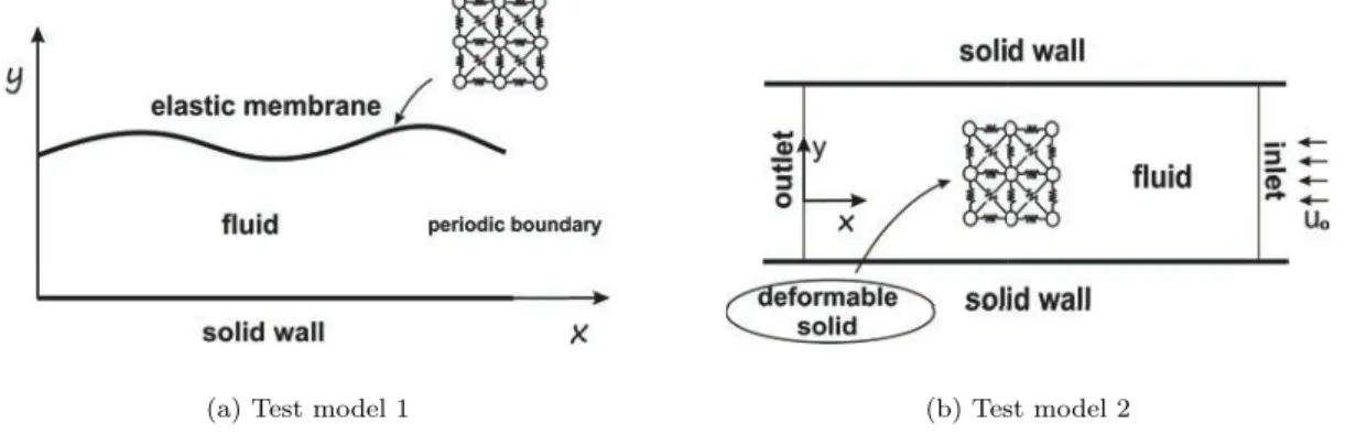
The purpose of this paper is to make a simple fluid-solid interaction with volume preservation for the solid, by using MPS and mass spring model. Several models have been proposed to handle this kind of interaction [5] [3], including those using MPS and mass-spring system [13]. However, our model is different in the way we handle the mass-spring system. Through this model we simulate the motion of a membrane with external force applied from above (see Figure 1a) and the deformation and motion of a box inside parallel flow (Figure 1b).

(a) Test model 1 (b) Test model 2

Figure 1: Test models.

2 MPS in Computational Fluid Dynamics (CFD)

Finite difference method (FDM), finite volume method (FVM) and finite element method FEM are very powerful, popular and widely used methods in CFD. In these methods, continuum domain is discretized into a fixed discrete grid or mesh. The strategy with fixed grids assures both robustness and accuracy when obtaining the solution of a differential equation using the discrete system. How- ever, this strategy also gives several limitations in analyzing complex geometries and multiphysics problems, which consequently limits the application of these methods to practical problems. The limitations of the fixed grid and mesh-based methods have triggered the development of a mesh free method which uses only a set of distributed nodes to express the mechanical system in a discretized form. The particle method developed for incompressible flow is called moving particle semi-implicit (MPS). In the MPS method, fluids are represented by a set of moving particles and governing equations are discretized by particle interaction models, hence grids are not necessary.

2.1 Governing Equations

Governing equations express the conservation laws of mass and momentum, 1

ρ

∂ρ

∂t + ∇ · u = 0, (1)

Du Dt = − 1

ρ ∇ P + v ∇

u + f, (2)

while incompressible fluids must satisfy

∂ρ

∂t = 0.

Here ρ denotes density, P pressure, v viscosity, u velocity and f external force. The left-hand side of Eq.(2) is the Lagrangian time differentiation involving advection terms. In MPS methods advection terms are directly incorporated into the calculation of moving particles. In this study, we solve two-dimensional problems and the only outer force considered is the gravity [9]. The Navier-Stokes solution process by MPS is a semi-implicit prediction-correction process. Namely, the basic Eq.(2) is divided into two parts,

( Du Dt

)

= υ ∇

u + f (3)

and (

Du Dt

)

= − 1

ρ ∇ P. (4)

We solve Eq.(3) first to predict the velocity and position of fluid particles. Therefore, in the first part the accelerations of the particles taking into account all the terms except for pressure are evaluated, and the temporal velocities and positions are calculated by

u

= u

+ ∆t ( Du

Dt

)

r

= r

+ ∆tu

.

The pressure term Eq.(4) is included by solving Poisson equation for pressure in the second part of the algorithm. The velocities and positions of each particle are modified as

u

= u

+ ∆t ( Du

Dt

)

r

= r

+ ∆t

( Du

Dt

)

.

2.2 Particle Interaction Model

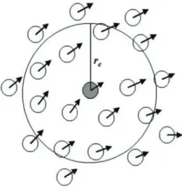
A particle interacts with its neighboring particles within the support of weight function w(r), where r is a distance between two particles. The weight function employed in this study has the following form

w(r) = {

e

r

− 1 0 ≤ r < r

0 r

≤ r.

Hence, a particle interacts with only a finite number of particles located within the distance of r

. The cutoff radius r

limits the number of the neighboring particles and allows to reduce the computational cost. The accuracy may be deteriorated with few neighbor particles when we adopt an excessively small radius. On the other hand, a larger radius will make the spatial resolution lower [6].

To calculate the weighted average, a normalization factor called particle number density be- tween particle i and its neighbors j located at positions r

and r

is used:

h n i

= ∑

j6=1

w( | r

− r

| ). (5)

Figure 2: Particle interaction given by weight function.

This value is assumed to be proportional to the density. As the density is almost constant in incompressibility calculation, we use the constant n

instead of h n i

in the formulation of weighted average.

The gradient operator is modeled using the weight function. A gradient vector between two neighboring particles i and j is evaluated as (φ

- φ

)(r

− r

) / | r

− r

|

, where φ is a physical quantity. The gradient vector at r

is then a weighted average of these vectors :

h∇ φ i

= d n

∑

j6=i

(φ

− φ

)

| r

− r

|

(r

− r

)w( | r

− r

| ), (6) where d is the number of space dimensions and n

is the reference value of the particle number density. In Eq.(6) a different value φ

is used in place of φ

because of stability reasons. If the configuration of neighboring particles is isotropic, Eq.(6) is not sensitive to absolute value and any value can be used for φ

. However, the configuration is not isotropic in general. In that case, the value of φ

in this study is calculated by

φ

= min φ

for { j | w( | r

− r

| ) 6 = 0 } .

This means that the minimum value is selected among the neighboring particles within the distance of r

. Using Eq.(6), forces between particles are always repulsive because φ

− φ

is positive. As noted in [6], this contributes to numerical stability.

Laplacian operator is modeled by the following identity:

h∇

φ i

= 2d λn

∑

j6=i

(φ

− φ

)w( | r

− r

| ).

Here, the parameter λ is introduced so that the variance increase is equal to the analytical solution, which yields

λ =

∑

j6=i

| r

− r

|

w( | r

− r

| )

∑

j6=i

w( | r

− r

| ) .

3 Mass Spring Model

The mass-spring model is an array of masses linked by springs. Each mass connects to its adjacent masses as in the figure below. The movement of each mass is determined by the spring force and damp force between the masses.

Figure 3: Basic mass-spring model.

The spring force complies with the Hooke’s law. Supposed there are springs connecting the mass i with its neighbors denoted by Ω. According to Hooke’s law, the spring force is written as

F

= − ∑

j∈Ω

k

( | l

| − l

) l

| l

| ,

and the damp force has the form

F

= − ∑

j∈Ω

b

(v

− v

),

where k

is the stiffness of the spring, l

is the rest length of the spring, b

is the coefficient of elasticity of the spring between the masses i and j, l

is the vector connecting neighboring masses and v

is the speed of the mass i.

According to Newton’s second law of motion, the total force on each node (mass) is F

= F

+ F

+ F

,

where F

is the external force that also influences the movement of nodes.

To solve this equation the Verlet method is used. Beginning at a time step n and given position r

, velocity v

and force F

acting on each node, the following equations are used to obtain values for the next step [11].

v

2

= v

+ ∆t 2 m

F

r

= r

+ v

2

∆t F

= F (r

) + F

+ F

v

= v

+ ∆t

2 m

F

.

4 Volume Preservation

During deformable solid object simulation we need to keep its volume constant to maintain relia- bility of our model. Here we adopt the method of [4]. The idea is to use the divergence theorem to transform the expression for the volume of the solid body to an integral over the surface of the body. This integral is then evaluated using a triangular mesh for the surface and there is no need to analyze the structure of the whole object.

The condition of total volume preservation is cast into a constrained dynamic system. The constrained formulation using Lagrange multipliers results in a mixed system of ordinary differential equations and algebraic expressions. The system of equations is represented using dn generalized coordinates q, where n is the number of discrete masses. The generalized coordinates which are simply the Cartesian coordinates of the discrete masses are defined in our 2D setting as

q = [x

, y

, x

, y

, . . . , x

, y

]

.

The difference between V

(original volume) and V (current volume) should be 0 for each iteration process, which is written using the constraint function Φ(q, t) as follows:

Φ(q, t) = V − V

= 0.

To maintain the volume at a constant value, implicit method is applied. The equation of motion and kinematic relationship between q and ˙ q are discretized in the following way:

q(t ˙ + ∆t) = ˙ q(t) − ∆tM

∇ Φ(q, t)λ + ∆tM

F

(q, t), (7)

q(t + ∆t) = q(t) + ∆t q(t ˙ + ∆t). (8)

Here F

are spring forces acting on the discrete masses, M is a dn × dn diagonal matrix containing discrete nodal masses, λ is a Lagrange multiplier, and ∇ Φ = ∇

V . We treat the constrained equations at new time implicitly,

Φ(q(t + ∆t), t + ∆t) = 0. (9)

Eq. (9) is now approximated using a truncated first-order Taylor series:

Φ(q, t) + ∇ Φ

(q, t)(q(t + ∆t) − q(t)) + Φ

(q, t)∆t = 0. (10) Substituting ˙ q(t + ∆t) from Eq. (7) into Eq. (8) we obtain

q(t + ∆t) = q(t) + ∆t q(t) + (∆t) ˙

{ M

F

(q, t) − M

∇ Φ(q, t)λ } . (11) Substituting this result into Eq. (10) results in the following identity, which yields the Lagrange multiplier by a simple division:

∇ Φ

(q, t)M

∇ Φ(q, t)λ = 1

∆t

Φ(q, t) + 1

∆t Φ

(q, t) + ∇ Φ

(q, t)( 1

∆t q(t) + ˙ M

F

(q, t)). (12)

5 Weak Coupling of Fluid and Solid

In this simulation the interaction between the fluid and the solid is carried out in the manner of

weak coupling, where the effect of the fluid on the solid is calculated after one iteration of the fluid

[13]. Steps of the interaction between the fluid and the solid are described as follows.

1. Determine the motion of fluid particles for one calculation step using the MPS method with time step ∆t

.

2. Calculate the fluid force F

, consisting of pressure and viscous force acting on each solid particle i that interacts with fluid:

F

= F

+ F

,

where F

= m

(

)

(without considering external force f ), and F

= m

(

)

.

3. Determine the motion of the solid particles using the spring network model for time ∆t

. This amounts to solving the set of equations of motion with respect to the solid particles,

m

r ¨

+ b

( ˙ r

− r ˙

) = F

+ F

(13) with the Verlet method. Here, the dot denotes the time derivative, j is a neighbor of the solid particle i and F

includes the spring forces and volume constraint. Since the time step

∆t

used in mass spring calculation is different from the time step ∆t

, the motion of solid was calculated for ∆t

/∆t

iterative steps.

4. Return to step 1 and repeat procedures 1. - 4. until the final time is reached.

6 Results and Discussion

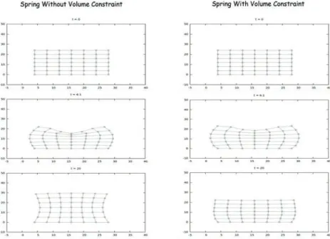
First, we tested the mass spring and volume preservation model using a 7 × 7 mass spring system with the configuration of springs as in Figure 3. The response of the object was compared for the cases with and without volume constraint after applying an external force from above for a period of time and then releasing it. The difference is shown in Figure 4 and Figure 5 shows the evolution of the relative volume error computed by the formula

ε = V − V

V

.

Next, we tested the fluid-solid interaction model using two problems (Figure 6). In the first computation, the upper part of a two-dimensional tube corresponds to a deformable solid wall and acts like a membrane, while the the bottom part is considered as a rigid wall. External force is applied on the upper wall from above for a period of time. Solid deformations due to the external force cause oscillations of the membrane. This vibration triggers an interaction between fluid and solid and a flow is observed inside the tube. In order to preserve tube’s volume, we connected the bottom and upper part with a spring. In this way, the whole domain is included in the mass-spring system and the volume is thus preserved. For the upper membrane, 3 × 39 nodes are used.

In the second test problem, both upper and lower part of the tube are rigid walls, while we

insert a deformable solid object inside the tube. The boundary condition on the inlet is selected as

uniform velocity U

in the negative x-direction Here we use 9 × 5 nodes to approximate the box,

which deforms into a parachute-like shape, while being transported by the fluid flow.

Figure 4: Mass spring model without and with volume preservation.

Figure 5: Relative error of volume during the simulation.

7 Conclusion

We have succeeded in simulating a simple fluid-solid interaction by use of the Moving Particle

Semi-implicit method for fluid flow and mass-spring system for solid deformation keeping the

volume constant throughout the simulation process. The key of the model is a weak coupling

Figure 6: Results of test problems.

interaction between the fluid and the solid, where the effect of viscosity and pressure count as the external forces for mass-spring system after one fluid iteration. We use a smaller time steps for solid calculations then for fluid calculations. To be able to simulate a real part of a human body like in [13] or [5], parameter tuning and increase in resolution are indispensable.

References

[1] H.-J. Bungartz, M. Sch¨ afer (2006). Fluid-structure Interaction: Modelling, Simulation, Opti- mization, Springer-Verlag.

[2] D. Bourguignon, M.-P. Cani. Controlling anisotropy in mass-spring systems, Eurographics Workshop on Computer Animation and Simulation (EGCAS), 113–123.

[3] O. Genevaux, A. Habibi, J.H. Dischler. Simulating fluid-solid interacion, LSIIT UMR CNRS- ULP 7005.

[4] M. Hong, S. Jung, M.H. Choi, S.W.J. Welch (2006). Fast Volume Preservation for a Mass- Spring System, IEEE Computer Graphics and Applications 26(5), 83–91.

[5] M. Kazama, S. Omata (2009). Modeling and computation of fluid-membrane interaction, Non-

linear Analysis 71, e1553-e1559.

[6] M. Kondo, S. Koshizuka (2011). Improvement of stability in moving particle semi-implicit method, Int. J. Numer. Meth. Fluids 65, 638?-654.

[7] S. Koshizuka, Y. Oka (1995). A particle method for incompressible viscous flow with fluid fragmentation, Comput. Fluid Dyn. J. 4 (1), 29-46.

[8] S. Koshizuka, Y. Oka (1996). Moving particle semi-implicit method for fragmentation of in- compressible fluid, Nucl. Sci. Eng. 123 (3), 421-434.

[9] S. Koshizuka, A. Nobe , Y. Oka (1998). Numerical Analysis of Breaking Waves Using The Moving Particle Semi-Implicit Method, International Journal for Numerical Methods in Fluids 26, 751-769.

[10] S. Koshizuka (2005). Moving Particle Semi-Implicit (MPS) Method : A Particle Method for Fluid and Solid Dynamics, in IACM expressions. Bulletin for The International Association for Computational Mechanics, 4–9.

[11] J. Li, D. Zhang, G. Lu, Y. Peng, X. Wen, Y. Sakaguti (2005). Flattening Triangulated Surfaces Using a Mass-Spring Model, Int. J. Adv. Manuf. Technol. 25, 108–117.

[12] G.S.P.Miller (1988). The motion dynamics of snakes and worms, SIGGRAPH 88 Confrence Proceedings, 198 – 178.

[13] K. Tsubota, S. Wada, T. Yamaguchi (2006). Particle method for computer simulation of red

blood cell motion in blood flow, Computer Methods and Programs in Biomedicine 83, 139–146.