Downloadedfromhttp://journals.lww.com/investigativeradiologybyBhDMf5ePHKav1zEoum1tQfN4a+kJLhEZgbsIHo4XMi0hCywCX1AWnYQp/IlQrHD31sQqFNBnHAeZDBuAnga2gjZRpGm4+XqPxKLX4kJ9yBU=on02/15/2019
Downloadedfrom
http:
//journals.
lww.com/
investigat iveradiologyby
BhDMf
5ePHK av1zEoum1t
QfN4a+
kJLhEZ gbsIHo4X Mi0hCywCX1A WnY
Qp/
IlQ
rHD31sQqF NBnHA eZDB uAnga2gjZ RpGm4+
XqP
xKLX 4kJ9yBU=
on02/
15/2019
Linearity, Bias, Intrascanner Repeatability, and Interscanner Reproducibility of Quantitative Multidynamic Multiecho
Sequence for Rapid Simultaneous Relaxometry at 3 T
A Validation Study With a Standardized Phantom and Healthy Controls
Akifumi Hagiwara, MD,*† Masaaki Hori, MD, PhD,* Julien Cohen-Adad, PhD,*‡§ Misaki Nakazawa, MS,*
Yuichi Suzuki, PhD,† Akihiro Kasahara, PhD,† Moeko Horita, BS,*|| Takuya Haruyama, BS,*||
Christina Andica, MD,* Tomoko Maekawa, MD,*† Koji Kamagata, MD, PhD,*
Kanako Kunishima Kumamaru, MD, PhD,* Osamu Abe, MD, PhD,† and Shigeki Aoki, MD, PhD*
Objectives:The aim of this study was to evaluate the linearity, bias, intrascanner repeatability, and interscanner reproducibility of quantitative values derived from a multidynamic multiecho (MDME) sequence for rapid simultaneous relaxometry.
Materials and Methods:The NIST/ISMRM (National Institute of Standards and Technology/International Society for Magnetic Resonance in Medicine) phantom, containing spheres with standardized T1 and T2 relaxation times and proton density (PD), and 10 healthy volunteers, were scanned 10 times on different days and 2 times during the same session, using the MDME sequence, on three 3 T scanners from different vendors. For healthy volunteers, brain volumetry and myelin estima- tion were performed based on the measured T1, T2, and PD. The measured phan- tom values were compared with reference values; volunteer values were compared with their averages across 3 scanners.
Results:The linearity of both phantom and volunteer measurements in T1, T2, and PD values was very strong (R2= 0.973–1.000, 0.979–1.000, and 0.982–0.999, re- spectively) The highest intrascanner coefficients of variation (CVs) for T1, T2, and PD were 2.07%, 7.60%, and 12.86% for phantom data, and 1.33%, 0.89%, and 0.77% for volunteer data, respectively. The highest interscanner CVs of T1, T2, and PD were 10.86%, 15.27%, and 9.95% for phantom data, and 3.15%, 5.76%, and 3.21% for volunteer data, respectively. Variation of T1 and T2 tended to be larger at higher values outside the range of those typically observed in brain tissue.
The highest intrascanner and interscanner CVs for brain tissue volumetry were 2.50% and 5.74%, respectively, for cerebrospinal fluid.
Conclusions:Quantitative values derived from the MDME sequence are overall robust for brain relaxometry and volumetry on 3 T scanners from different ven- dors. Caution is warranted when applying MDME sequence on anatomies with relaxometry values outside the range of those typically observed in brain tissue.
Key Words:SyMRI, synthetic MRI, quantitative MRI, brain, relaxometry, automatic brain segmentation, myelin estimation
(Invest Radiol2018;54: 39–47)
I
n clinical practice, T1-, T2-, and fluid-attenuated inversion recovery, and other contrast-weighted magnetic resonance imaging (MRI) scans are assessed on the basis of relative signal differences. The signal intensity depends on sequence parameters and scanner settings, but also on B0 and B1 inhomogeneity, coil sensitivity profiles, and RF amplifica- tion settings, making quantitative comparisons difficult. Tissue relaxometry is a more direct approach to obtaining scanner-independent values. Ab- solute quantification of tissue properties by relaxometry has been re- ported in research settings for characterization of disease,1assessment of disease activity,2and monitoring of treatment effect.3A number of methods have been proposed for simultaneous relaxometry of T1 and T2,4–7but due to the additional scanning time required, these methods had not been widely introduced into clinical practice.Recently, a multidynamic multiecho (MDME) sequence for rapid simultaneous measurement of T1 and T2 relaxation times and proton density (PD), with correction of B1 field inhomogeneity, was proposed for full head coverage within approximately 6 minutes,8and has shown promising results on 1.5 T and 3 T scanners in healthy subjects9and pa- tients with multiple sclerosis (MS),10brain metastases,11Sturge-Weber syndrome,12and bacterial meningitis.13These quantitative values allow postacquisition generation of any contrast-weighted image via synthetic MRI, obviating the need for additional conventional T1-weighted and T2-weighted imaging required in routine clinical settings.14The acquired maps are inherently aligned, thus avoiding potential errors due to image coregistration for multiparametric quantification of a certain area. In ad- dition, brain tissue volumes,15including myelin,16can be automatically calculated and potentially used to assess brain tissue loss associated with normal aging, neuroinflammatory, or neurodegenerative diseases.17,18 Myelin estimation based on the MDME sequence has shown high repeat- ability19and good correlation with histological measures in postmortem human brain20and with other myelin estimation methods.21
According to the Quantitative Imaging Biomarkers Alliance of the Radiological Society of North America, 3 metrology criteria are critical to the performance of a quantitative imaging biomarker: accuracy (linearity and bias), repeatability, and reproducibility.22Previous studies evaluated T1, T2, and PD values acquired with the MDME sequence on a 1.5 T
Received for publication May 24, 2018; and accepted for publication, after revision, July 27, 2018.
From the *Department of Radiology, Juntendo University School of Medicine;
†Department of Radiology, Graduate School of Medicine, The University of Tokyo, Tokyo, Japan;‡NeuroPoly Lab, Institute of Biomedical Engineering, Polytechnique Montreal; §Functional Neuroimaging Unit, CRIUGM, Université de Montréal, Montreal, Quebec, Canada; and ||Department of Radiological Sciences, Graduate School of Human Health Sciences, Tokyo Metropolitan University, Tokyo, Japan.
Conflicts of interest and sources of funding: This work was supported by AMED under grant number JP18lk1010025; ImPACT Program of Council for Science, Technology, and Innovation (Cabinet Office, Government of Japan); JSPS KAKENHI grant number 16K19852; JSPS KAKENHI grant num- ber JP16H06280, Grant-in-Aid for Scientific Research on Innovative Areas–
Resource and Technical Support Platforms for Promoting Research“Advanced Bioimaging Support”; and the Japanese Society for Magnetic Resonance in Med- icine. The authors declare no conflict of interest.
Supplemental digital contents are available for this article. Direct URL citations appear in the printed text and are provided in the HTML and PDF versions of this article on the journal’s Web site (www.investigativeradiology.com).
Correspondence to: Akifumi Hagiwara, MD, Department of Radiology, Juntendo University School of Medicine, 1-2-1, Hongo, Bunkyo-ku, Tokyo, Japan, 113-8421.
E-mail: [email protected].
Copyright © 2018 The Author(s). Published by Wolters Kluwer Health, Inc. This is an open-access article distributed under the terms of the Creative Commons Attribution-Non Commercial-No Derivatives License 4.0 (CCBY-NC-ND), where it is permissible to download and share the work provided it is properly cited. The work cannot be changed in any way or used commercially without permission from the journal.
ISSN: 0020-9996/19/5401–0039 DOI: 10.1097/RLI.0000000000000510
O RIGINAL A RTICLE
Investigative Radiology • Volume 54, Number 1, January 2019 www.investigativeradiology.com 39
【別添】
scanner, by assessing accuracy,23,24repeatability,24and reproducibil- ity using different head coils.24 However, to our knowledge, no study has compared quantitative values acquired with the MDME sequence on different scanners.
The aim of this study was to evaluate linearity, bias, intrascanner repeatability, and interscanner reproducibility of quantitative values de- rived from the MDME sequence using three 3 T scanners all from dif- ferent vendors. In addition, we investigated the robustness of brain tissue volume measurements made using the MDME sequence.
MATERIALS AND METHODS MR Acquisition and Postprocessing
The MDME sequence was performed on GE Healthcare (Discov- ery 750w, Milwaukee, WI), Siemens Healthcare (MAGNETOM Prisma, Erlangen, Germany), and Philips (Ingenia, Best, the Netherlands) 3 T scanners (scannerα,β, andγ, respectively). This sequence is a mul- tislice, multisaturation delay, multiecho, fast spin-echo sequence, using combinations of 2 echo times and 4 delay times to produce 8 complex images per slice. To retrieve T1, T2, and PD maps while accounting for B1 inhomogeneity, a least square fit was performed on the signal inten- sity (I) of these images by minimizing the following equation:
I¼A:PD:expð−TE=T2Þ1−f1−cosðB1θÞgexpð−TI=T1Þ−cosðB1θÞexpð−TR=T1Þ 1−cosðB1αÞcosðB1θÞexpð−TR=T1Þ
whereαis the applied excitation flip angle 90 degrees andθis the sat- uration flip angle of 120 degrees. A is an overall intensity scaling factor that takes into account several elements, including sensitivity of the coil, amplification of the radiofrequency chain, and voxel volume.
The details of the sequence composition and postprocessing are de- scribed elsewhere.23The postprocessing was performed using SyMRI software (version 8.0; SyntheticMR AB, Linköping, Sweden), resulting in T1, T2, and PD maps. The characteristics of the 3 scanners and the detailed acquisition parameters of the MDME sequence are shown in Supplementary Table 1 and Supplementary Table 2 (both in Supple- mental Digital Content 1, http://links.lww.com/RLI/A400) for phan- tom and volunteer studies, respectively. We used the predetermined parameters provided by each vendor without any change. For volun- teers, 3-dimensional (3D) T1-weighted images were also acquired on scanner α. The acquisition parameters of the 3D T1-weighted inversion-recovery spoiled gradient echo images were as follows: repe- tition time, 7.6 milliseconds; echo time, 3.09 milliseconds; inversion time, 400 milliseconds; bandwidth, 244 Hz/pixel; thickness, 1 mm;
field of view, 256$256 mm; matrix size, 256$256; acquisition time, 5 minutes 45 seconds.
Phantom Study
The NIST/ISMRM (National Institute of Standards and Technology/International Society for Magnetic Resonance in Medicine) MRI system phantom (High Precision Devices, Inc, Boulder, CO), consisting of multiple layers of sphere arrays with known T1, T2, and PD values, was used. Reference values, confirmed by magnetic reso- nance spectroscopy, were provided by NIST.25,26 The T1 and T2 spheres were filled with NiCl2 and MnCl2 solutions, respectively.
We selected 6 T1 spheres and 10 T2 spheres with T1 and T2 values within the clinically relevant dynamic range (300–4300 milliseconds and 20–2000 milliseconds, respectively). All 14 PD spheres from the phantom were used in the study. The PD spheres consisted of different concentrations of water (H2O) and heavy water (D2O). The container of the phantom was filled with distilled water. The reference values for T1, T2, and PD at 20°C are shown in Supplementary Table 3 (Supplemental Digital Content 1, http://links.lww.com/RLI/A400).
The phantom was scanned 10 times each on scannersα,β, and γover a 2-month period, with an interval of at least 1 day between con- secutive scans. The phantom was placed for 30 minutes before each scan. The temperature of the phantom was 20°C ± 1°C, measured after each scan.
A circular region of interest of 1.150 cm2was placed in the cen- ter of each sphere on T1, T2, and PD maps using OsiriX Imaging Soft- ware, Version 7.5 (http://www.osirix-viewer.com), to include as much of the sphere as possible while avoiding partial volume with the edge.
Regions of interest on all the spheres were simultaneously copied and pasted on the data acquired at different times, and the mean values were recorded.
Volunteer Study
This study was approved by the institutional review boards, and written informed consent was acquired from all participants. Ten healthy volunteers (3 men; mean age, 24.7 years; age range, 21–32 years) were included. None of the participants had a history of a major medical condition, neurological or psychiatric disorder, and all had normal structural MRIs.
Each participant was scanned twice during each session on scan- nersα,β, andγ(in that order) over a 1-week period, with sessions at least 1 day apart. The subjects were removed from the scanner after the first scan and repositioned for the second scan.
T1, T2, and PD maps were acquired for all participants and proc- essed using SyMRI software8to obtain gray matter (GM), white matter (WM), and cerebrospinal fluid (CSF) segmentation, volumetry of brain tissues, and myelin estimation. Tissue volume fractions were calculated for each voxel. Voxels not categorized as GM, WM, or CSF were clas- sified as other brain material (NoN). Myelin volume fraction (MVF) in
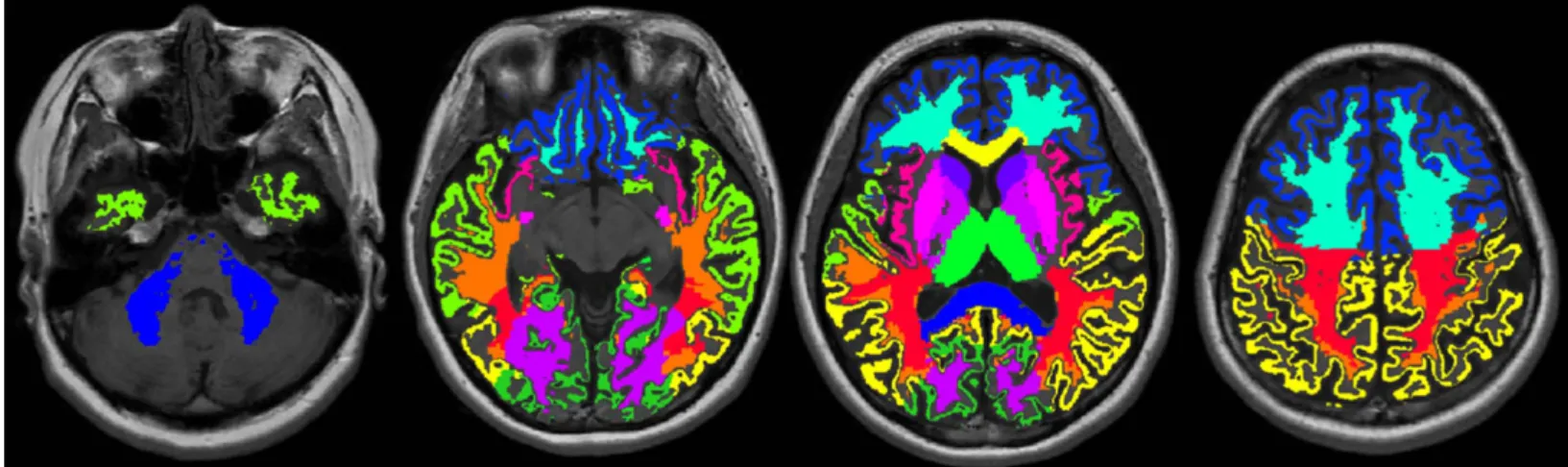
FIGURE 1. Example of volume of interest measurement. Volumes of interest are overlaid on T1-weighed images.
Hagiwara et al Investigative Radiology • Volume 54, Number 1, January 2019
40 www.investigativeradiology.com © 2018 Wolters Kluwer Health, Inc. All rights reserved.
each voxel was estimated based on a 4-compartment model,16using T1, T2, and PD values of myelin, excess parenchymal water, cellular water, and free water partial volumes. The 4-compartment model assumes that the relaxation behavior of each compartment contributes to the effective relaxation behavior of each voxel, while considering the magnetization exchange rates between partial volume compartments. The details of brain segmentation and myelin estimation are described elsewhere.15,16 The total volumes of GM, WM, CSF, NoN, and myelin (MYV) were calculated by multiplying the aggregated volume fraction of each tissue type and the voxel volume.15,16The brain parenchymal volume (BPV) was calculated as the sum of GM, WM, and NoN. The borderline of in- tracranial volume (ICV) was defined at points where PD = 50%.27
T1, T2, PD, and MVF maps were used for the volume of interest (VOI) analysis. We created 16 VOIs: 8 GM (frontal, parietal, temporal and occipital GM, insula, caudate, putamen, and thalamus) and 8 WM (frontal, parietal, temporal and occipital WM, genu and splenium of corpus callosum, internal capsules, and middle cerebellar peduncles) VOIs in the Montreal Neurological Institute space. Other than those of splenium, VOIs from the left and right were combined for analysis.
Aggregate GM and WM VOIs were also created by combining these re- gional VOIs. Volume of interest analysis was performed using FMRIB Software Library (FSL, http://fsl.fmrib.ox.ac.uk/fsl/fslwiki/FSL). We transformed VOIs created in the Montreal Neurological Institute space to the space of each subject using the FSL linear and nonlinear image reg- istration tool (FLIRT and FNIRT), based on the synthetic T1-weighted (TR, 500; TE, 10) and 3D T1-weighted images. The GM and WM masks were generated from the synthetic T1-weighted images using FMRIB’s Automated Segmentation Tool (FAST). These masks were then thresholded at 0.9 and used on the T1, T2, PD, and MVF maps to com- pute average values within the GM and WM. Figure 1 shows an example of VOI measurements.
Statistical Analysis
Ten measurements of the spheres in the phantom were averaged for each of the 3 scanners. Linear regression was performed for these values versus the reference values. Bland-Altman analysis was per- formed to assess agreement between the reference values and those acquired on each scanner. Linear regression was also performed for the values from the first scans of volunteers on scannersα,β, andγver- sus the average values obtained from these scanners.
Coefficients of variation (CVs) were calculated within each scanner (intrascanner CV) and across scanners (interscanner CV). For the phantom study, the intrascanner CV was calculated based on the
10 scans. The interscanner CV was calculated using the average values from each of the 3 scanners. For the volunteer study, the intrascanner CVs were calculated per subject (based on the scan and rescan) and then averaged across subjects. Interscanner CVs were calculated for each subject using the data of the first scan, then averaged into a single interscanner CV value.
RESULTS Phantom Study
The temperature of the phantom after imaging was 19.76°C ± 0.23°C (mean ± SD) on scannerα, 20.06°C ± 0.59°C on scannerβ, and 19.57°C ± 0.28°C on scannerγ.
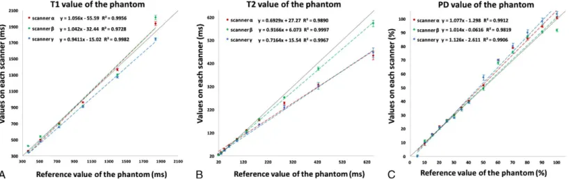
Figure 2 shows mean values of T1, T2, and PD acquired over 10 times on each scanner plotted against the known reference values. The regression analysis showed strong linear correlation (R2= 0.973–0.998 for T1;R2= 0.989–1.000 for T2;R2= 0.982–0.991 for PD).
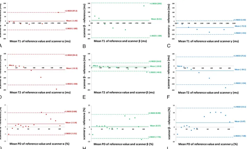
Figure 3 shows Bland-Altman plots for the values acquired on each scanner and the reference values of the phantom. Overall, trends of biases for T1, T2, and PD showed similar patterns across different vendors. All data points were within the 95% limits of agreement, except the longest T1 value (reference value, 1838 milliseconds) on scannerα, the longest T2 value (reference value, 645.8 milliseconds) on all scanners, 1 PD point (reference value, 60%) for scannerα, and the highest PD value (reference value, 100%) for scannerβ. Higher T1 and T2 values outside the range of those observed in the brain tissue (see Supplementary Table 4, Supplemental Digital Content 1, http://
links.lww.com/RLI/A400) showed greater bias. On the other hand, PD values less than 60% (reference value), which were outside the range of values observed in the brain tissue, showed smaller bias than higher PD values, except PD 5% (reference value), which was measured as 0%
on all 3 scanners.
Table 1 shows the intrascanner and interscanner CV of phantom T1, T2, and PD measurements. The highest intrascanner CV of T1 values was 2.07% (scannerβ). Intrascanner CVs of T2 values were less than 4.25% on scannersαandβ, and less than 7.60% on scannerγ;
those of PD values were less than 3.71%, except the CV for a PD refer- ence value of 10%, which was 12.86% on scannerα, and for a PD ref- erence value of 100%, which was 5.13% on scannerβ.
The interscanner CV was higher than intrascanner CV for all ranges of T1 (3.25%–10.86%), T2 (4.28%–15.27%), and PD (1.35%–9.95%) values, except PD 10% (reference value). Within the range of brain tissue properties (see Supplementary Table 4, Supplemental Digital Content 1, http://links.lww.com/RLI/A400),
FIGURE 2. Scatterplots showing linearity of measured T1 (A), T2 (B), and proton density (C) values of the NIST/ISMRM phantom averaged across 10 acquisitions, plotted against reference values. Error bars represent one standard deviation. Dashed lines represent linear regression fits (red for scannerα, green for scannerβ, and blue for scannerγ), whereas the solid lines represent identity.
Investigative Radiology • Volume 54, Number 1, January 2019 Reliability of SyMRI at 3 T
© 2018 Wolters Kluwer Health, Inc. All rights reserved. www.investigativeradiology.com 41
TABLE 1. Mean Values of All Measurements and Their Intrascanner and Interscanner CV on the NIST/ISMRM Phantom for T1, T2, and PD
T1 Scannerα Scannerβ Scannerγ T2 Scannerα Scannerβ Scannerγ
Sphere No.
Mean ± SD, ms
Intrascanner CV, %
Intrascanner CV, %
Intrascanner CV, %
Interscanner CV, %
Mean ± SD, ms
Intrascanner CV, %
Intrascanner CV, %
Intrascanner CV, %
Interscanner CV, %
1 376 ± 40.9 0.96 1.01 0.50 10.86 22.7 ± 3.25 1.26 1.18 7.60 14.28
2 506 ± 31.8 0.98 2.07 0.77 6.29 32.9 ± 3.77 1.05 0.91 5.90 11.44
3 682 ± 22.4 0.70 1.16 1.14 3.28 45.9 ± 3.25 1.05 0.95 5.27 7.09
4 930 ± 30.2 0.71 0.97 0.67 3.25 63.7 ± 2.87 1.02 0.85 4.71 4.51
5 1324 ± 49.6 1.02 1.33 0.73 3.77 89.4 ± 3.83 1.38 0.90 4.48 4.28
6 1897 ± 138 1.21 1.31 0.92 7.27 127 ± 5.81 1.69 0.90 3.71 4.59
7 171 ± 12.0 1.87 1.14 1.76 7.05
8 251 ± 21.4 2.79 1.21 4.01 8.53
9 350 ± 41.2 2.99 1.69 4.45 11.79
10 505 ± 77.0 4.25 2.45 4.64 15.27
11 12 13 14
For PD value 5% (reference value), measurement yielded 0% on all scanners, so CV was not calculated.
CV indicates coefficient of variation; PD, proton density; SD, standard deviation.
FIGURE 3. Bland-Altman plots showing bias of measurements of T1 (A, for scannerα; B, for scannerβ; and C, for scannerγ), T2 (D, for scannerα; E, for scannerβ; and F, for scannerγ), and proton density (G, for scannerα; H, for scannerβ; and I, for scannerγ) for the NIST/ISMRM phantom.
Hagiwara et al Investigative Radiology • Volume 54, Number 1, January 2019
42 www.investigativeradiology.com © 2018 Wolters Kluwer Health, Inc. All rights reserved.
PD Scannerα Scannerβ Scannerγ Mean ± SD, %
Intrascanner CV, %
Intrascanner CV, %
Intrascanner CV, %
Interscanner CV, %
0 N/A N/A N/A N/A
10.0 ± 1.00 12.86 2.38 1.37 9.95
15.9 ± 0.21 1.24 1.05 0.66 1.35
21.2 ± 0.60 1.09 1.03 0.86 2.83
25.8 ± 0.45 1.84 1.41 1.05 1.75
29.2 ± 1.10 1.68 0.40 1.52 3.76
34.5 ± 0.89 1.49 1.45 1.11 2.59
39.6 ± 0.56 1.31 1.37 1.32 1.42
52.7 ± 4.27 1.06 1.11 3.71 8.11
69.4 ± 1.26 0.76 3.50 1.11 1.82
78.3 ± 2.31 0.62 1.36 2.72 2.95
87.4 ± 2.36 1.23 0.73 2.56 2.70
94.3 ± 3.83 0.73 1.20 2.59 4.06
98.7 ± 6.26 0.98 5.13 1.73 6.35
FIGURE 4. Scatterplots showing linearity of measured T1 (A), T2 (B), proton density (C), and myelin volume fraction (D) values of the brains of healthy volunteers, plotted against averaged values across all 3 scanners. Only the data of the first acquisition was used. Dashed lines represent linear regression fits (red for scannerα, green for scannerβ, and blue for scannerγ), whereas the solid lines represent identity.
Investigative Radiology • Volume 54, Number 1, January 2019 Reliability of SyMRI at 3 T
© 2018 Wolters Kluwer Health, Inc. All rights reserved. www.investigativeradiology.com 43
interscanner CVs of T1 (645–1280 milliseconds) were less than 6.3%, interscanner CV of T2 (61.9–79.6 milliseconds) was 4.51%
and interscanner CVs of PD (58.9–84.8 milliseconds) were less than 3.0%.
Volunteer Study
Figure 4 shows T1, T2, PD, and MVF values for the first acqui- sition on each scanner plotted against the mean of the 3 scanners. The regression analysis showed strong linear correlation (R2= 0.999–1.000 for T1; R2 = 0.979–0.993 for T2; R2 = 0.999–0.999 for PD; R2 = 0.999–0.999 for MVF).
Supplementary Table 4 (Supplemental Digital Content 1, http://
links.lww.com/RLI/A400) shows the intrascanner and interscanner CVs of T1, T2, PD, and MVF, and the values for aggregate GM and WM VOIs are extracted and shown in Table 2. The highest intrascanner CVs of T1, T2, PD, and MVF were 1.33%, 0.89%, 0.77%, and 4.56%, respectively, across all VOIs. The interscanner CV was higher than the intrascanner CV for all ranges of T1, T2, PD, and MVF (1.06%–3.15%, 3.61%–5.76%, 0.68%–3.21%, and 2.53%–14.6%, respectively).
Figure 5 shows volumetric data (GM, WM, CSF, NoN, BPV, ICV, MYV) for the first acquisition on each scanner plotted against the mean of the 3 scanners. The regression analysis showed strong linear correla- tion for GM, WM, CSF, BPV, ICV, and MYV (R2 = 0.966–0.999).
NoN showed a weaker linear correlation (R2= 0.791–0.856).
Table 3 shows the intrascanner and interscanner CVs of volumet- ric data from the 3 scanners. The intrascanner CVs were 0.11% to 1.17% for GM, WM, BPV, ICV, and MYV, 0.16 to 2.50% for CSF, and 3.43% to 10.8% for NoN. The interscanner CVs were in the range 0.42% to 5.74% for all measures except NoN (16.3%), and thus higher than the corresponding intrascanner CVs for all tissue volumes.
DISCUSSION
In this study, we evaluated linearity, bias, intrascanner repeatabil- ity, and interscanner reproducibility of multiple quantitative values ac- quired by the MDME sequence, with 3 scanners from different vendors, in both standardized NIST/ISMRM phantom and 10 healthy volunteers. Although the phantom study showed some bias with respect to the reference values, linearity was very strong in all the measure- ments, indicating that the MDME sequence can differentiate materials with different tissue properties. Trends of biases for T1, T2, and PD shown as Bland-Altman plots were similar in the 3 scanners, which could also demonstrate the robustness of the MDME sequence even across different vendors.
The T1, T2, and PD values acquired in vivo in our study fell in the same order of magnitude as those reported in previous studies using 3 T scanners,6,28–31which reported a wide range of T1 and T2 values (eg, T1 600–1100 milliseconds, T2 50–80 milliseconds, and 67%–73% in the
WM) for healthy controls, largely depending on the choice of acquisition method. To date, only a few studies have investigated interscanner repro- ducibility of specific MR relaxometry methods for human subjects across different vendors. Bauer et al32demonstrated that T2 values quantified with dual echo fast spin-echo on scanners from 3 different vendors showed variability up to 20%, and Deoni et al33validated driven equilib- rium single pulse observation of T1 and T2 with interscanner CVs of ap- proximately 6.5% and 8% for scanners from 2 different vendors. The results of our volunteer study (T1, highest CV 3.15%; T2, highest CV 5.60%) were comparable or better, even with different acquisition param- eters and coils across scanners to reflect daily radiological practice.
The intrascanner and interscanner CVs in our study were lower than the changes in T1 and PD values of normal-appearing brain tissue in patients with MS34,35and in the T2 values of the limbic system in pa- tients with Alzheimer disease.36Our results suggest that MDME se- quence could thus be of clinical value in multicenter and longitudinal studies, taking disease-specific within-group variation into account.37
The intrascanner CVs of T1, T2, and PD measurements in volun- teer data were very low (less than 1.4%) and lower than those in phan- tom data. However, the variation in phantom data acquired over 10 days could be partly explained by day-to-day variation in scanner perfor- mance, whereas the volunteers were scanned twice in the same session on the same day. In addition, the size of the region of interest used in phantom study was much smaller than those of the VOIs used in volun- teer study. Thus, we cannot simply compare the results of the volunteers and the phantom studies. Notably, interscanner CVs of T1 and T2 values in phantom data outside the range of the volunteer data were mostly higher than those of T1 and T2 values within the volunteer data range. These results could be attributed to the fact that the MDME se- quence was developed for the analysis of the brain tissue, and the com- mercial version of the MDME sequence may not have been fully optimized for materials with different relaxation properties.
The T2 measurements showed larger interscanner CV than those of T1. Every vendor uses their own RF pulse shapes and specific ab- sorption rate reduction models to decrease the 180-degree refocusing pulses during the TSE readout. This could also explain the differences in the intrascanner CVs of the T2 measurements across scanners, with scannerγshowing higher values than scannersαandβ. Moreover, the B1 inhomogeneity profiles differ per scanner and even per object, and imperfect gradient refocusing due to eddy currents may decrease signal intensity. These factors affect the signal amplitude during the multiecho readout, potentially resulting in an apparently altered T2 relaxation. In the postprocessing, RF pulse shape, B1 amplitude, and B1 inhomoge- neity are taken into account and corrected for, but this may not be per- fect. It should be noted that long T2 times were mainly affected, beyond the typical T2 values of brain tissue, suggesting that T2 measurement of CSF would be less reliable. To improve the interscanner CVof T2, more echoes than the current 2 could potentially be added to the sequence, TABLE 2. Mean Values in the GM and WM Based on the First Scan on 3 Scanners and Intrascanner and Interscanner CV of T1, T2, PD, and MVF for 3 Scanners Averaged Across 10 Subjects
T1 Scannerα Scannerβ Scannerγ T2 Scannerα Scannerβ Scannerγ
VOI Mean, ms
Intrascanner CV, %
Intrascanner CV, %
Intrascanner CV, %
Interscanner CV, %
Mean ± SD, ms
Intrascanner CV, %
Intrascanner CV, %
Intrascanner CV, %
Interscanner CV, % Aggregate
GM VOIs 1062 ± 23.3 0.51 ± 0.57 0.30 ± 0.24 0.43 ± 0.31 1.33 ± 0.54 73.3 ± 2.80 0.57 ± 0.43 0.20 ± 0.11 0.60 ± 0.64 4.15 ± 0.36 Aggregate
WM VOIs 725 ± 21.8 0.67 ± 0.62 0.38 ± 0.23 0.52 ± 0.53 1.89 ± 0.62 69.0 ± 2.94 0.52 ± 0.40 0.26 ± 0.12 0.37 ± 0.29 4.63 ± 0.31 Values are mean ± SD. Size of the VOIs are also shown in the last column.
CV indicates coefficient of variation; GM, gray matter; PD, proton density; SD, standard deviation; VOI, volume of interest; WM, white matter.
Hagiwara et al Investigative Radiology • Volume 54, Number 1, January 2019
44 www.investigativeradiology.com © 2018 Wolters Kluwer Health, Inc. All rights reserved.
PD Scannerα Scannerβ Scannerγ MVF Scannerα Scannerβ Scannerγ Mean ±
SD, %
Intrascanner CV, %
Intrascanner CV, %
Intrascanner CV, %
Interscanner CV, %
Mean ± SD, %
Intrascanner CV, %
Intrascanner CV, %
Intrascanner CV, %
Interscanner CV, %
Size of VOI, cm3 77.2 ± 1.13 0.15 ± 0.17 0.12 ± 0.09 0.12 ± 0.11 1.20 ± 0.30 16.4 ± 1.54 0.68 ± 0.60 0.63 ± 0.50 0.76 ± 0.44 5.76 ± 1.13 492 ± 41.1 63.3 ± 1.25 0.36 ± 0.32 0.22 ± 0.10 0.32 ± 0.29 1.55 ± 0.32 33.9 ± 1.91 1.11 ± 1.07 0.64 ± 0.30 0.81 ± 0.75 4.46 ± 0.82 240 ± 26.8
FIGURE 5. Scatterplots showing linearity of volumetric measurements of gray matter (A), white matter (B), cerebrospinal fluid (C), other brain materials (D), brain parenchymal volume (E), intracranial volume (F), and myelin volume (G) of the volunteer brains, plotted against the average of the values across all 3 scanners. Only the data of the first acquisition was used. Dashed lines represent linear regression fit (red for scannerα, green for scannerβ, and blue for scannerγ), whereas the solid lines represent identity.
Investigative Radiology • Volume 54, Number 1, January 2019 Reliability of SyMRI at 3 T
© 2018 Wolters Kluwer Health, Inc. All rights reserved. www.investigativeradiology.com 45
but this would increase the total scan time, which would be detrimental for introduction of the sequence into clinical routine. Application of the MDME sequence to objects other than the brain has been reported for T2 measurement of musculoskeletal tissue.38–40Although the MDME and multiecho spin-echo sequence showed good agreement with each other for T2 measurement of phantom, knee cartilage, and muscle, mean T2 value of bone marrow measured by multiecho spin-echo was significantly higher than that measured by the MDME sequence.38 This discrepancy was assumed to be because of the varying contribu- tions from water and lipid protons, which resulted in multiexponential decay.39 The quantitative values acquired by the MDME sequence should be cautiously assessed when used to other tissues than brain.
We also observed low interscanner and intrascanner CVof tissue volumes calculated using the T1, T2, and PD maps acquired by the MDME sequence. The interscanner CVs of all tissue volumes were higher than the intrascanner CVs, reflecting the higher interscanner CVs of T1, T2, and PD measurements. Our intrascanner CVs were comparable to those reported in previous studies using 3D T1- weighted images acquired on 1.5 T and 3 T scanners based on various segmentation algorithms.41–44Further, our interscanner CVs for GM, WM, CSF, BPV, and ICV were slightly lower than those shown by Huppertz et al43for a single subject using 3D T1-weighted images ac- quired on 6 scanners with field strength of 1.5 T and 3 T. The NoN vol- ume, which is the smallest compartment, showed the highest variability among all types of tissue volume, consistent with previous reports.15,19,45 Granberg et al45showed lower intrascanner CV of NoN volume in MS patients than in healthy controls, indicating clinical utility of NoN volume as measures of lesion load. The algorithm implemented in the SyMRI software only uses quantitative values of each voxel for segmentation,15 and utilization of structural information, by, for example, a deep learning approach,46might further improve the segmentation.
The repeatability of MVF in healthy volunteer data was high, with the intrascanner CVs lower than 4.6%, but higher than those of T1, T2, and PD, probably reflecting small errors in measurement of each quanti- tative value. The interscanner reproducibility of MVF in the WM was overall higher than that in the GM, with the highest interscanner CVs being 6.67% and 14.60%, respectively. The intrascanner CV of MVF in WM was slightly lower than the results reported (1.3%–2.4%) by Nguyen et al47for the myelin water fraction in WM. To our knowledge, no previous study has evaluated the interscanner reproducibility of my- elin imaging for different vendors.
There are some limitations to our study. First, we only used 3 T scanners, hence our results cannot be generalized to scanners with dif- ferent field strength. Second, we did not include patients with any brain disease. A cerebral lesion would affect T1, T2, and PD values and
consequently the repeatability and reproducibility measurements.
Hagiwara et al10showed focal MS plaques in the WM to have mean T1 value of 1111 milliseconds, T2 value of 91.9 milliseconds, and PD value of 78.86% using the MDME sequence on a 3 T MR scanner.
In our study using the phantom, intrascanner and interscanner CV at these T1, T2, and PD values were at the same order of magnitude as the range of T1, T2, and PD in the normal WM, indicating that the MDME sequence may reliably be used in the evaluation of WM demyelinating lesions.
In conclusion, brain quantitative values derived from the MDME sequence at 3 T are overall robust even across different scanners. Cau- tion is warranted when applying MDME sequence to anatomies with different relaxation properties compared with brain tissue.
REFERENCES
1. West J, Aalto A, Tisell A, et al. Normal appearing and diffusely abnormal white matter in patients with multiple sclerosis assessed with quantitative MR.PLoS One.
2014;9:e95161.
2. Horsthuis K, Nederveen AJ, de Feiter MW, et al. Mapping of T1-values and gadolinium-concentrations in MRI as indicator of disease activity in luminal Crohn's disease: a feasibility study.J Magn Reson Imaging. 2009;29:488–493.
3. Wagner MC, Lukas P, Herzog M, et al. MRI and proton-NMR relaxation times in diagnosis and therapeutic monitoring of squamous cell carcinoma.Eur Radiol.
1994;4:314–323.
4. Ma D, Gulani V, Seiberlich N, et al. Magnetic resonance fingerprinting.Nature.
2013;495:187–192.
5. Newbould RD, Skare ST, Alley MT, et al. Three-dimensional T(1), T(2) and pro- ton density mapping with inversion recovery balanced SSFP.Magn Reson Imaging.
2010;28:1374–1382.
6. Ehses P, Seiberlich N, Ma D, et al. IR TrueFISP with a golden-ratio-based radial readout: fast quantification of T1, T2, and proton density.Magn Reson Med.
2013;69:71–81.
7. Deoni SC, Rutt BK, Arun T, et al. Gleaning multicomponent T1 and T2 informa- tion from steady-state imaging data.Magn Reson Med. 2008;60:1372–1387.
8. Hagiwara A, Warntjes M, Hori M, et al. SyMRI of the brain: rapid quantification of relaxation rates and proton density, with synthetic MRI, automatic brain seg- mentation, and myelin measurement.Invest Radiol. 2017;52:647–657.
9. Lee SM, Choi YH, You SK, et al. Age-related changes in tissue value properties in children: simultaneous quantification of relaxation times and proton density using synthetic magnetic resonance imaging.Invest Radiol. 2018;53:236–245.
10. Hagiwara A, Hori M, Yokoyama K, et al. Utility of a multiparametric quantitative MRI model that assesses myelin and edema for evaluating plaques, periplaque white matter, and normal-appearing white matter in patients with multiple sclero- sis: a feasibility study.AJNR Am J Neuroradiol. 2017;38:237–242.
11. Hagiwara A, Hori M, Suzuki M, et al. Contrast-enhanced synthetic MRI for the detection of brain metastases.Acta Radiol Open. 2016;5:2058460115626757.
12. Hagiwara A, Nakazawa M, Andica C, et al. Dural enhancement in a patient with Sturge-Weber syndrome revealed by double inversion recovery contrast using syn- thetic MRI.Magn Reson Med Sci. 2016;15:151–152.
TABLE 3. Mean of All Volumetric Measurements Based on the First Scan, and the Intrascanner and Interscanner CV of Volunteers for GM, WM, CSF, NoN, BPV, ICV, and MVF
Scannerα Scannerβ Scannerγ
Tissue Type Mean, mL Intrascanner CV, % Intrascanner CV, % Intrascanner CV, % Interscanner CV, %
GM 727 ± 48.1 1.10 ± 0.90 0.50 ± 0.44 0.99 ± 0.72 2.94 ± 1.22
WM 537 ± 61.3 1.15 ± 1.04 0.54 ± 0.52 1.11 ± 0.69 2.40 ± 1.30
CSF 136 ± 37.0 2.50 ± 1.00 0.16 ± 0.10 1.22 ± 0.80 5.74 ± 2.36
NoN 18.2 ± 5.3 10.8 ± 17.4 3.43 ± 3.39 5.63 ± 3.62 16.3 ± 6.76
BPV 1282 ± 96.1 0.40 ± 0.64 0.11 ± 0.10 0.25 ± 0.16 0.73 ± 0.40
ICV 1418 ± 121 0.33 ± 0.47 0.11 ± 0.10 0.18 ± 0.12 0.42 ± 0.17
MYV 179 ± 25.0 1.17 ± 1.01 0.70 ± 0.52 1.06 ± 0.85 5.20 ± 1.11
Values are mean ± SD.
CV indicates coefficient of variation; GM, gray matter; WM, white matter; CSF, cerebrospinal fluid; NoN, other brain material; BPV, brain parenchymal volume; ICV, intracranial volume; MYV, myelin volume.
Hagiwara et al Investigative Radiology • Volume 54, Number 1, January 2019
46 www.investigativeradiology.com © 2018 Wolters Kluwer Health, Inc. All rights reserved.
13. Andica C, Hagiwara A, Nakazawa M, et al. Synthetic MR imaging in the diagno- sis of bacterial meningitis.Magn Reson Med Sci. 2017;16:91–92.
14. Blystad I, Warntjes JB, Smedby O, et al. Synthetic MRI of the brain in a clinical setting.Acta Radiol. 2012;53:1158–1163.
15. West J, Warntjes JB, Lundberg P. Novel whole brain segmentation and volume estimation using quantitative MRI.Eur Radiol. 2012;22:998–1007.
16. Warntjes M, Engström M, Tisell A, et al. Modeling the presence of myelin and edema in the brain based on multi-parametric quantitative MRI.Front Neurol.
2016;7:16.
17. Jack CRJr, Shiung MM, Gunter JL, et al. Comparison of different MRI brain atrophy rate measures with clinical disease progression in AD. Neurology.
2004;62:591–600.
18. Miller DH, Barkhof F, Frank JA, et al. Measurement of atrophy in multiple scle- rosis: pathological basis, methodological aspects and clinical relevance.Brain.
2002;125(pt 8):1676–1695.
19. Andica C, Hagiwara A, Hori M, et al. Automated brain tissue and myelin volumetry based on quantitative MR imaging with various in-plane resolutions.
J Neuroradiol. 2018;45:164–168.
20. Warntjes JBM, Persson A, Berge J, et al. Myelin detection using rapid quantitative MR imaging correlated to macroscopically registered luxol fast blue-stained brain specimens.AJNR Am J Neuroradiol. 2017;38:1096–1102.
21. Hagiwara A, Hori M, Kamagata K, et al. Myelin measurement: comparison be- tween simultaneous tissue relaxometry, magnetization transfer saturation index, and T1w/T2w ratio methods.Sci Rep. 2018;8:10554.
22. Raunig DL, McShane LM, Pennello G, et al. Quantitative imaging biomarkers: a review of statistical methods for technical performance assessment.Stat Methods Med Res. 2015;24:27–67.
23. Warntjes JB, Leinhard OD, West J, et al. Rapid magnetic resonance quantification on the brain: optimization for clinical usage.Magn Reson Med. 2008;60:320–329.
24. Krauss W, Gunnarsson M, Andersson T, et al. Accuracy and reproducibility of a quantitative magnetic resonance imaging method for concurrent measurements of tissue relaxation times and proton density.Magn Reson Imaging. 2015;33:584–591.
25. Russek S, Boss M, Jackson E, et al. Characterization of NIST/ISMRM MRI System Phantom. In:In Proceedings of the 20th Annual Meeting of ISMRM.
Melbourne, Victoria, Austraia; 2012: Abstract 2456.
26. Keenan K, Stupic K, Boss M, et al Multi-site, multi-vendor comparison of T1 measurement using ISMRM/NIST system phantom. In:Proceedings of the 24th Annual Meeting of ISMRM. Singapore; 2016: Abstract 3290.
27. Ambarki K, Lindqvist T, Wahlin A, et al. Evaluation of automatic measurement of the intracranial volume based on quantitative MR imaging.AJNR Am J Neuroradiol. 2012;33:1951–1956.
28. Stikov N, Boudreau M, Levesque IR, et al. On the accuracy of T1 mapping:
searching for common ground.Magn Reson Med. 2015;73:514–522.
29. McPhee KC, Wilman AH. Transverse relaxation and flip angle mapping: evalua- tion of simultaneous and independent methods using multiple spin echoes.Magn Reson Med. 2017;77:2057–2065.
30. Whittall KP, MacKay AL, Graeb DA, et al. In vivo measurement of T2 distributions and water contents in normal human brain.Magn Reson Med. 1997;37:34–43.
31. Abbas Z, Gras V, Mollenhoff K, et al. Analysis of proton-density bias corrections based on T1 measurement for robust quantification of water content in the brain at 3 Tesla.Magn Reson Med. 2014;72:1735–1745.
32. Bauer CM, Jara H, Killiany R, et al. Whole brain quantitative T2 MRI across mul- tiple scanners with dual echo FSE: applications to AD, MCI, and normal aging.
Neuroimage. 2010;52:508–514.
33. Deoni SCL, Williams SCR, Jezzard P, et al. Standardized structural magnetic res- onance imaging in multicentre studies using quantitative T1 and T2 imaging at 1.5 T.Neuroimage. 2008;40:662–671.
34. Davies GR, Hadjiprocopis A, Altmann DR, et al. Normal-appearing grey and white matter T1 abnormality in early relapsing-remitting multiple sclerosis: a lon- gitudinal study.Mult Scler. 2007;13:169–177.
35. Reitz SC, Hof SM, Fleischer V, et al. Multi-parametric quantitative MRI of normal appearing white matter in multiple sclerosis, and the effect of disease activity on T2.Brain Imaging Behav. 2017;11:744–753.
36. Wang H, Yuan H, Shu L, et al. Prolongation of T(2) relaxation times of hippocam- pus and amygdala in Alzheimer's disease.Neurosci Lett. 2004;363:150–153.
37. Tofts PS. Measurement in MRI. In: Cercignani M, Dowell NG, Tofts PS, eds.
Quantitative MRI of the Brain. 2nd ed. Boca Raton, FL: CRC Press; 2018:10–11.
38. Park S, Kwack KS, Lee YJ, et al. Initial experience with synthetic MRI of the knee at 3T: comparison with conventional T1 weighted imaging and T2 mapping.Br J Radiol. 2017;90:20170350.
39. Chougar L, Hagiwara A, Andica C, et al. Synthetic MRI of the knee: new perspec- tives in musculoskeletal imaging and possible applications for the assessment of bone marrow disorders.Br J Radiol. 2018;91:20170886.
40. Lee SH, Lee YH, Song HT, et al. Quantitative T2 mapping of knee cartilage: com- parison between the synthetic MR imaging and the CPMG sequence.Magn Reson Med Sci. 2018. [Epub ahead of print].
41. Landman BA, Huang AJ, Gifford A, et al. Multi-parametric neuroimaging repro- ducibility: a 3-T resource study.Neuroimage. 2011;54:2854–2866.
42. Sampat MP, Healy BC, Meier DS, et al. Disease modeling in multiple sclerosis:
assessment and quantification of sources of variability in brain parenchymal frac- tion measurements.Neuroimage. 2010;52:1367–1373.
43. Huppertz HJ, Kroll-Seger J, Kloppel S, et al. Intra- and interscanner variability of automated voxel-based volumetry based on a 3D probabilistic atlas of human ce- rebral structures.Neuroimage. 2010;49:2216–2224.
44. de Boer R, Vrooman HA, Ikram MA, et al. Accuracy and reproducibility study of automatic MRI brain tissue segmentation methods. Neuroimage. 2010;51:
1047–1056.
45. Granberg T, Uppman M, Hashim F, et al. Clinical feasibility of synthetic MRI in multiple sclerosis: a diagnostic and volumetric validation study. AJNR Am J Neuroradiol. 2016;37:1023–1029.
46. Akkus Z, Galimzianova A, Hoogi A, et al. Deep learning for brain MRI segmen- tation: state of the art and future directions.J Digit Imaging. 2017;30:449–459.
47. Nguyen TD, Deh K, Monohan E, et al. Feasibility and reproducibility of whole brain myelin water mapping in 4 minutes using fast acquisition with spiral trajec- tory and adiabatic T2prep (FAST-T2) at 3T.Magn Reson Med. 2016;76:456–465.
Investigative Radiology • Volume 54, Number 1, January 2019 Reliability of SyMRI at 3 T
© 2018 Wolters Kluwer Health, Inc. All rights reserved. www.investigativeradiology.com 47
JournalofNeuroradiology47(2020)134–135
Availableonlineat
ScienceDirect
www.sciencedirect.com
Editorial
Synthetic MRI and MR fingerprinting in routine neuroimaging protocol: What’s the next step?
Simultaneousrelaxometrytechniquestomaprelaxationparam- etersin tissuesareattracting widespreadinterestowingtothe objectivequantificationoftissuepropertiesandpotentialreduction inthescantime.Sofar,syntheticMRIandMRfingerprinting(MRF) arethetwomajorsimultaneousrelaxometrytechniqueswithregu- latoryapproval.SyntheticMRImapsT1andT2relaxationtimesand protondensityandsynthesizesvariouscontrast-weightedimages, including T1- and T2-weighted and fluid-attenuated inversion recovery(FLAIR)imageswithinasingle6-minacquisition[1–3].
MRFisanother promising approach tosimultaneouslyquantify tissuepropertiesinaclinicallyfeasibletime.Insteadofperform- ingcurvefitting,asinconventionalrelaxometrytechniques,MRF adoptsa unique approach in which acquisition parameters are simultaneously varied across repetition times to generate sig- nalevolutionsthatcharacterizethevariousrelaxationprocesses uniquetoeachtissue[4].Theacquiredsignalispattern-matchedto adictionaryofsimulatedsignalevolutionstoacquirevariousquan- titativemetrics,suchasT1andT2values.BothsyntheticMRIand MRFshowhighrepeatabilityandreproducibilityofT1andT2val- uesforstandardizedphantoms[5–7]andinvivo[6–9].Moreover, recenteffortshaveenabledhigh-resolutionthree-dimensionalvol- umecoverageofthewholebrainonbothsyntheticMRI[10,11]and MRF[12–14].Inaddition,accelerationtechniques,suchassimul- taneousmulti-sliceacquisition [15],have beenimplementedto furtheracceleratescanning,makingtheserelaxometrytechniques moreusableinclinicalsettings.
InthisissueofJournalofNeuroradiology,Ryuetal.reportedtheir initialexperiencewithcontrast-weightedimagesobtainedusing syntheticMRIasaroutineneuroimagingprotocolindailyclinical practice[16].Contrarytomanypreviousstudiesthatusedsyn- theticMRIintheresearchprotocol,thisstudywasuniqueinthat itimplementedsyntheticMRIastheroutineprotocolbyreplacing someconventionalsequences,suchasT1andT2-weightedimages, withsyntheticMRI.Tworadiologistsretrospectivelyreviewedthe imagingdataof89patients,ratedtheoverallimagequalityand anatomicaldelineation,andfoundthattheimagequalitiesofsyn- theticT1-andT2-weightedimageswereadequateforclinicaluse.
FLAIRimagesshowedpronouncedartifactsbutwithoutanysignif- icantimpactonthediagnosis.Further,theyalsoevaluatedimages obtainedwithsyntheticphase-sensitiveinversionrecovery(PSIR), whichisa T1-weightedsequencewithagreatersignalintensity range,andfoundthattheoverallimagequalitywithanatomical delineationofPSIRwassuperiortothatofothersyntheticimages.
TheyconcludedthatsyntheticMRIcanbeacceptedasaroutine neuroimagingprotocolintheclinicalpractice.
Then, why have synthetic MRI and MRF not been widely acceptedintheclinics,despitetheirpotentialandpromisingper- formance reported in the literature? A major challenge is the generationof high-quality synthetic imagesfromthe quantita- tivemaps.Ingeneral,thequalityofFLAIRimagesgeneratedfrom quantitativerelaxation maps is inferiorto that of conventional FLAIRimages,whichisanessentialsequenceinneuroradiology.
Although Ryuet al. [16] and previousstudies [17,18]reported thattheinferiorqualityofsyntheticFLAIRimagesdidnotaffect thediagnosticability,cliniciansmaynotbeconfidentregarding itsuseyet.Theacquisitionisrapid,butadding thesequenceto theprotocolwillprolongthetotalscantime.Toimplementsyn- theticMRIorMRFinatime-limitedclinicalworkflow,someexisting sequencesshouldbereplacedsothattheentireprotocolisnotelon- gated.Hence,improvementoftheimagesynthesistechniqueto generatehigh-qualitycontrast-weightedimageswouldbeakey stepforawideclinicalimplementation.Approachesthatrelyon amulti-componentmodelmaypotentiallymitigateartifactsseen onsyntheticFLAIRimages[19].Adoptingdeeplearningtodirectly generate contrast-weighted imageswhile bypassing T1 and T2 maps hasalso been gathering considerableinterest for several years[20–22].ThisapproachimprovestheFLAIRimagequalityand, furthermore,generatesMRangiographyimages, which arealso importantintheclinicalpractice.Implementationofthesetech- niquesisexpectedtofurtheracceleratetheuseofsyntheticMRI andMRFintheroutineclinicalpractice.
Disclosureofinterest
Theauthorsdeclarethattheyhavenocompetinginterest.
Grantsupport
This work was supported by JSPS KAKENHI grant num- ber 18H02772and 19K17177;and AMEDunder grant number 19dm0307101h0001.
References
[1].WarntjesJB, LeinhardOD,WestJ,LundbergP.Rapidmagnetic resonance quantificationonthebrain:optimizationforclinicalusage.MagnResonMed.
2008;60(2):320–329.
[2].AndicaC,HagiwaraA,HoriM,KamagataK,KoshinoS,MaekawaT,etal.Review ofsyntheticMRIinpediatricbrains:basicprincipleofMRquantification,itsfea- tures,clinicalapplications,andlimitations.JNeuroradiol.2019;46(4):268–275.
[3].HagiwaraA,WarntjesM,HoriM,AndicaC,NakazawaM,KumamaruKK,etal.
SyMRIofthebrain:rapidquantificationofrelaxationratesandprotondensity, https://doi.org/10.1016/j.neurad.2020.02.001
0150-9861/©2020ElsevierMassonSAS.Allrightsreserved.