Gas Diffusion Coefficient in Unsaturated Peat Soil: Measurements, Development and Tests of Predictive Models

論文 

不飽和泥炭土のガス拡散係数の測定と予測モデルの構築・検証 Gas Diffusion Coefficient in Unsaturated Peat Soil:

Measurements, Development and Tests of Predictive Models 川本 健

^*

, 海野将孝

^*

，飯塚健仁

^*

，小松登志子

^*

Ken KAWAMOTO, Masataka UNNO, Kenji IIDUKA, and Toshiko KOMATSU

The soil-gas diffusion coefficient (D

_p

) and its dependency on air-filled porosity (ε) govern the gas diffusion and reaction processes in soil. Accurate D

_p

(ε) prediction models for unsaturated saturated peat soils are needed to evaluate vadose zone transport and fate of greenhouse gases such as methane in peaty wetlands.

In this study, we measured D

_p

on peat soil samples at different pF conditions, and developed new expressions for describing and predicting D

_p

(ε). Undisturbed peat soil samples were taken from Bibai wetland, Hokkaido, Japan. By modifying existing D

_p

(ε) models, the Buckingham model and the Macroporosity-Dependent model, we suggested two new D

_p

(ε) models for peat soils. To validate the new D

p

(ε) models, we tested the models against independent datasets for peat soil samples from literatures. The modified Buckingham type model performed the best against independent datasets.

Keywords: Soil-Gas Diffusion Coefficient, Peat Soil, Air-Filled Porosity, Predictive Model

1.

  はじめに

ラムサール条約（

1971

年）に代表されるように湿地 の保全は強く求められている。日本や欧米諸国では周 辺環境との調和を考慮した，いわゆる環境共生型の開 発・保全事業が積極的に行われている。一方で，湿地 は開発途上国においては重要な開発（農地・宅地・社 会基盤整備）候補地であり，急速な湿地開発が行われ ている。湿地は，固有生態系を形成する貴重な自然財 産であるのみならず，高い洪水調整機能や水質浄化機 能を有するが，同時に還元的な湿地環境は温室効果ガ スであるメタン放出を促進するといった負の側面も有

する。さらに，湿地開発における客土や排水は，広大 な周辺領域の地盤沈下を引き起こす。このように，湿 地の環境共生型開発・保全事業の計画には，湿地およ びその周辺環境における物質循環・地盤工学的挙動の 適切な把握が極めて重要な課題となる。

湿地を構成する土壌は，一般に高有機質であり，そ の代表例として植物遺体が未分解のまま堆積した泥炭 土が挙げられる。泥炭土は高い間隙率（概ね

0.8

以上）

を有することから，通常の鉱物土壌と比較して，非常 にユニークな物質移動特性や力学特性を示すことが知 られている^{1), 2)}。しかし，これまでの泥炭土研究は飽和 状態での泥炭土の透水性や圧密挙動に注目したものが 大半であり，不飽和泥炭土のガス移動に関する研究は 少ない。地表面直下に存在する不飽和泥炭土は，地中 の飽和泥炭土（地下水面下）と大気との間に存在し，

水・ガス・エネルギー（熱）といった物質交換が直接 的に行なわれる場であり，湿地における物質循環を考

*

埼玉大学  大学院理工学研究科 

Graduate School of Science and Engineering, Saitama University, 255 Shimo-Okubo, Sakura-ku, Saitama, Saitama, 338-8570, Japan

（原稿受付日：平成 21 年5月29日） 

 

BIBAI

Peat 3 (G.W.L.60cm)

Peat 1 (G.W.L.5‐10cm) Peat 2 (G.W.L.30‐40cm)

BIBAI

Peat 3 (G.W.L.60cm)

Peat 1 (G.W.L.5‐10cm) Peat 2 (G.W.L.30‐40cm)

える際に重要な境界となる。

本研究では，不飽和泥炭土の物質移動の中でも，特 にガス拡散に注目した。ガス拡散は不飽和土壌内にお けるガス移動を支配する重要なメカニズムであり，ガ ス拡散移動量の大小を決定する土壌ガス拡散係数（

D

p） は，湿地表層と大気の間のガス交換や，温室効果ガス の放出を予測・評価する際に必要となる。本研究では，

試料として北海道美唄湿地より採取した泥炭土を用い て，不飽和水分状態における

D

pを測定した。これらの 測定データに基づき既存の

D

予測モデルを修正し，不 飽和泥炭土に適用し得る新たな

D

p予測モデルを提案し た。さらに，新たな

D

p予測モデルの有効性を，文献デ ータを用いて検証した。

2.

  試料と実験

２

.

１ 泥炭土と試料特性

Fig. 1 Sampling points at Bibai wetland, Hokkaido, Japan.

本研究に使用した泥炭試料（Peat 1）は，北海道の美 唄湿原内（中央付近，Fig. 1）より採取した。美唄湿原 は東西約440m，南北約550mの湿原であり，その周囲は 農地化されている。近年は周辺排水路の影響により，

地下水位が湿原の辺縁部で顕著に低下し，湿原の北側 ではササ群落およびウルシ群落の侵入が確認されてい る。土壌ガス拡散係数用の不攪乱コア試料は，体積

100cm

³（高さ4.1cm，直径5.6cm）のコアサンプラーを

使用し，深さ0-30cmの6深さより，各2本ずつ採取した

（計12試料）．

後述する修正予測モデルの提案には，

Peat 1試料の他

に，同湿原内（西側排水路付近，Peat 2，12試料）なら びに同湿原に隣接する防風林内（Peat 3，

12試料）より

採取した不攪乱コア試料を用いて測定された土壌ガス 拡散係数データも用いた（Peat 1，

2， 3の位置関係はFig.

1を参照）

^{3), 4)}。各地点における泥炭土の基本物理化学

量をTable 1に示した。

２

.

２ 測定方法

不飽和泥炭土試料の水分調整および水分特性曲線の 測定は，サンドボックス法（吸引法）⁵⁾を用いて，飽和 からの脱水過程で行なった。設定pFは，

1.0， 1.5， 1.8，

2.0

の

4

段階とした。水分特性曲線の実測値に

Campbell

の水分特性モデル⁶⁾で回帰を行い，保水係数

b

を求めた。

土壌ガス拡散係数の測定は各水分状態に調整した試 料に対して行なった。測定は，遅沢⁷⁾やRolston and

Moldrup

⁸⁾の方法に従い，非定常法で行なった（Fig. 1）。 この方法は，コアサンプラーと連結した拡散容器に窒 素ガスを充填し，試料を通して大気と拡散ガスを相互 拡散させ，拡散容器内のガス（酸素）濃度変化を測定 する。所定の初期・境界条件で次のFickの第

2

法則を 解くことにより，土壌ガス拡散係数Dp（cm²

s

^-1）を決 定する。

2 p 2

x D C t C

∂

∂

= ε

∂

∂

     

[1]

ここで，

C :

拡散ガスの濃度 (g cm^-3

), ε :

気相率 (cm³

cm

^-3

)，x :

流れの方向距離 (cm)。

式(1)に対して，本測定装置の初期・境界条件（Fig. 2）

を用いて解いた解として，次式が得られる⁹⁾。

 

a 2

a 2 1 s

12 p a

i 0

i s

L / ) L / ( L

) / t D exp(

L 2 C C

C ) t L ( C

ε + ε

+ α

ε α ε −

− =

−

｝

｛

，

   

[2]

ここで，Ls

: 試料の高さ (cm)，L

a

: 拡散容器の高さ (cm)，C (L

s

, t) :

拡散容器中の拡散ガス濃度 (g cm^-3

)，

C

i

:

外気中の拡散ガス濃度 (g cm^-3

)，C

0

: t = 0

における 拡散容器内の拡散ガス濃度 (g cm^-3

)，α

1

: α tan(αL

s

)の 1

番目の正の根。

  実際のDpの算出にあたっては，ln {(Ct

- C

i

) / (C

0

- C

i

)}

を時間tに対してプロットし，得られた直線の傾き

-D

p

α

12

/εからD

_pを求めた．算出した土壌ガス拡散係数Dp

は，大気中における酸素のガス拡散係数Do

( = 2.04×10

^-1

cm

²

s

^-1

)との比をとり，相対土壌ガス拡散係数D

p

/D

oとし て評価した。

２

.

３ 予測モデルと実測データの適合性評価 ２

.

３ 予測モデルと実測データの適合性評価

土壌ガス拡散係数（Dp）の実測データと予測モデル との適合性評価には二乗平均平方根誤差（Root Mean

Square Error,

以下

RMSE

）とバイアス（

bias

）を用いた。

RMSE

は次式で表される。

土壌ガス拡散係数（D

RMSE=

RMSE=

p）の実測データと予測モデル との適合性評価には二乗平均平方根誤差（Root Mean

Square Error,

以下

RMSE

）とバイアス（

bias

）を用いた。

RMSE

は次式で表される。

∑

= n

1 i

i2

n d

1 [3]

ここで，

d

iは予測値と実測値との差，

n

は測定数である。

予測値と実測値との差が小さいほど

RMSE

は

0

に近く なり，両者の適合性が良いことを意味する。バイアス

は次式で表される。

bias= ∑

= n

1 i

d

i

n

1 [4]

バイアスの値が正の場合は，予測値が実測値を過大評 価し，逆に負の場合は予測値が実測値を過小評価して いることを示す。

Fig. 3 Initial and boundary conditions for calculating the soil-gas diffusion coefficient.

Sample

Diffusion chamber

O-ring

Oxygen electrode

Inlet and Outlet vulve

Slide plate Ls=

4.1cm

La= 9.5cm

Fig. 2 Experimental device for measuring the soil-gas diffusion coefficient. _t =0 t ＞0

0≤ x ＜ Ls x =0, C=C

i

C = C

i

0＜ x ≤ L

s

C =C (x,t ) L

s

＜ x ＜ L

s

+ L

a

L

s

≤ x ＜ L

s

+ L

a

C =C

0

C =C (L

s

,t ) x =0

x =L

s

x L

s

+L

a

試 料

拡散容器

=

Sample

Diffusion chamber

t =0 t ＞0

0≤ x ＜ Ls x =0, C=C

i

C = C

i

0＜ x ≤ L

s

C =C (x,t ) L

s

＜ x ＜ L

s

+ L

a

L

s

≤ x ＜ L

s

+ L

a

C =C

0

C =C (L

s

,t ) x =0

x L

s

x L

s

+L

a

試 料

拡散容器

=

=

Sample

Diffusion chamber Site depth

Particle Dry Bulk Gravimetric

Porosity Saturated Loss-on

SOC SON C/N Fiber content H*

dnsity density water content hydraulic conductivity -ignition

ρ_s ρ_d w φ Ks Li

(cm) (g/cm³) (g/cm³) (%) (cm³/cm³) (cm/s) (%) (%) (%) (%)

Peat 1

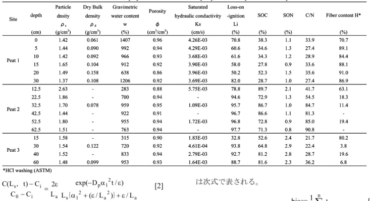
0 1.42 0.061 1407 0.96 4.26E-03 70.8 38.3 1.1 33.9 70.7 5 1.44 0.090 992 0.94 4.29E-03 60.6 34.6 1.3 27.4 89.1 10 1.42 0.092 966 0.93 3.68E-03 61.6 34.3 1.2 28.9 84.4 15 1.65 0.104 912 0.92 3.90E-03 58.0 27.8 0.9 33.6 88.1 20 1.49 0.158 638 0.86 3.96E-03 50.2 52.3 1.5 35.6 91.0 30 1.37 0.108 1206 0.92 3.69E-03 82.0 28.7 1.0 27.4 86.9

Peat 2

12.5 2.63 - 283 0.88 5.75E-03 78.8 89.7 2.1 41.7 63.1 22.5 1.86 - 700 0.94 - 94.6 72.9 1.3 54.5 18.3 32.5 1.70 0.078 959 0.95 1.09E-03 95.7 86.7 1.0 84.7 11.4 42.5 1.44 - 922 0.91 - 96.7 86.6 1.1 81.3 - 52.5 1.80 - 955 0.94 1.72E-03 96.8 72.8 0.9 85.0 19.4 62.5 1.51 - 763 0.94 - 97.7 71.3 0.8 90.8 -

Peat 3

15 1.58 - 315 0.90 1.83E-03 32.8 52.6 2.4 21.7 80.2 30 1.54 0.122 720 0.92 4.61E-04 93.8 64.8 2.9 22.4 3.8 40 1.52 - 833 0.94 2.79E-03 92.7 81.2 2.8 28.7 19.6 60 1.48 0.099 953 0.93 1.64E-03 88.7 81.6 2.3 36.2 6.8

*HCl washing (ASTM) Site depth

Particle Dry Bulk Gravimetric

Porosity Saturated Loss-on

SOC SON C/N Fiber content H*

dnsity density water content hydraulic conductivity -ignition

ρ_s ρ_d w φ Ks Li

(cm) (g/cm³) (g/cm³) (%) (cm³/cm³) (cm/s) (%) (%) (%) (%)

Peat 1

0 1.42 0.061 1407 0.96 4.26E-03 70.8 38.3 1.1 33.9 70.7 5 1.44 0.090 992 0.94 4.29E-03 60.6 34.6 1.3 27.4 89.1 10 1.42 0.092 966 0.93 3.68E-03 61.6 34.3 1.2 28.9 84.4 15 1.65 0.104 912 0.92 3.90E-03 58.0 27.8 0.9 33.6 88.1 20 1.49 0.158 638 0.86 3.96E-03 50.2 52.3 1.5 35.6 91.0 30 1.37 0.108 1206 0.92 3.69E-03 82.0 28.7 1.0 27.4 86.9

Peat 2

12.5 2.63 - 283 0.88 5.75E-03 78.8 89.7 2.1 41.7 63.1 22.5 1.86 - 700 0.94 - 94.6 72.9 1.3 54.5 18.3 32.5 1.70 0.078 959 0.95 1.09E-03 95.7 86.7 1.0 84.7 11.4 42.5 1.44 - 922 0.91 - 96.7 86.6 1.1 81.3 - 52.5 1.80 - 955 0.94 1.72E-03 96.8 72.8 0.9 85.0 19.4 62.5 1.51 - 763 0.94 - 97.7 71.3 0.8 90.8 -

Peat 3

15 1.58 - 315 0.90 1.83E-03 32.8 52.6 2.4 21.7 80.2 30 1.54 0.122 720 0.92 4.61E-04 93.8 64.8 2.9 22.4 3.8 40 1.52 - 833 0.94 2.79E-03 92.7 81.2 2.8 28.7 19.6 60 1.48 0.099 953 0.93 1.64E-03 88.7 81.6 2.3 36.2 6.8

*HCl washing (ASTM)

Table 1. Soil physical and chemical properties for peat soil samples.

 

３

.

１ 既存の予測モデル

土壌ガス拡散係数

D

pの予測モデルは，経験式10), 11), 12)

や理論式によるモデル¹³⁾，半理論式で表現されるモデ

ル^{14), 15)}など，これまで数多く提案されている。

Buckingham

モデル¹¹⁾は，間隙の連結度を表す指標

X

を用いて，次式で表される：

0 X p

/ D

D = ε [5]

ここで，εは気相率（

cm

³

cm

^-3）である。

X

は，実測デ ータから次式で算出される¹⁶⁾：

( )

( ) ε

= log D / D

X log

^{p 0}

[6]

一般鉱物土壌では，

X=2

となることが報告されている

11)。

 

Millington and Quirk (MQ)

モデル¹³⁾は最も普及してい るモデルであり，全間隙率φ （

cm

³

cm

^-3）を用いて，次 式で表される：

2 3 / 0 10 p

/ D /

D = ε φ

   

[7]

 

Macropore-dependent (MPD)モデル

¹⁵⁾は，ヨーロッパ 土壌

126

個の不攪乱試料のDpの実測データを基に構築 されたモデルである。基準気相率となるpF2.0における 気相率ε100（cm³

cm

^-3）との関係である[8]式とCampbell の保水係数bを用いて，[9]式のように記述される：

3 100 100 0 100 ,

p

/ D 2 0 . 04

D = ε + ε

     

[8]

 

D

_p

/ D

₀

= ( D

_p,100

/ D

₀

)( ε / ε

₁₀₀

)

^2+3b

[9]

３

.2

予測モデルの改良

本研究では，既存の予測モデルの中で，Buckingham モデルと

MPD

モデルを用いて，実測データを基に両 モデルに改良を加え，新たな

2

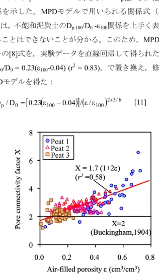
タイプの予測モデルを 提案した。

Fig. 4

に[6]式により得られたXとεの関係を示す。X

はεの増加とともに増加し，一般鉱物土壌におけるX=2 から大きく乖離することが分かる。このため，Xとεの

関数として扱い，その直線回帰式，X = 1.7(1+2ε) (r²

= 0.58)，を求めた。この回帰式を[5]式に代入すると，次

式が得られる：

) 2 1 ( 7 . 0 1 p

/ D

D = ε

^+ε

[10]

Fig. 5

には，

pF2.0

において測定された

D

p.100

/D

0とε₁₀₀の 関係を示した。

MPD

モデルで用いられる関係式（

[8]

式）は，不飽和泥炭土の

D

p.100

/D

0

-ε

₁₀₀関係を上手く表現 することはできないことが分かる。このため，

MPD

モ デルの

[8]

式を，実験データを直線回帰して得られた式，

D

p,100

/D

0

= 0.23(ε

₁₀₀

-0.04) (r

²

= 0.83)

，で置き換え，修正

MPD

モデルを得た：

( )

[

100

] (

100

)

^{2 3/b}

0

p

/ D 0 . 23 0 . 04 / /

D = ε − ε ε

⁺  

[11]

0 2 4 6 8

0.0 0.2 0.4 0.6 0.8 Air-filled porosity ε (cm

³

/cm

³

)

Pore con necti vit y factor X

X=2

(Buckingham,1904) Peat 1

Peat 2 Peat 3

X = 1.7 (1+2ε) (r

²

=0.58)

0 2 4 6 8

0.0 0.2 0.4 0.6 0.8 Air-filled porosity ε (cm

³

/cm

³

)

Pore con necti vit y factor X

X=2

(Buckingham,1904) Peat 1

Peat 2 Peat 3

X = 1.7 (1+2ε) (r

²

=0.58)

Fig. 4 Pore connectivity factor X as a function of ε.

0.0 0.1 0.2 0.3

0.0 0.2 0.4 0.6 0.8 D

p,100

/D

0

D

_p,100

/D

₀

=2ε

1003

+0.04ε

100

(MPD;

Moldrup et al., 2000)

Peat 1 Peat 2 Peat 3

ε

₁₀₀

(cm

³

/cm

³

)

D

_p,100

/D

₀

=0.23(ε

100

-0.04) (r

²

=0.75)

0.0 0.1 0.2 0.3

0.0 0.2 0.4 0.6 0.8 D

p,100

/D

0

D

_p,100

/D

₀

=2ε

1003

+0.04ε

100

(MPD;

Moldrup et al., 2000)

Peat 1 Peat 2 Peat 3

ε

₁₀₀

(cm

³

/cm

³

)

D

_p,100

/D

₀

=0.23(ε

100

-0.04) (r

²

=0.75)

Fig. 5 Soil-gas diffusivity (D

_p,100

/D

₀

) as a function of

air-filled porosity (ε

100

) at pF2.0.

 

本 研 究 で 新 た に 得 ら れ た 修 正

Buckingham

モ デ ル

（

[10]

式）と修正

MPD

モデル（

[11]

式）を，既往の研究 で報告されている高有機質土ならびに泥炭土の土壌ガ ス拡散係数のデータ15), 16), 17)に適用し，その有効性を検 討した。文献データの土壌特性を

Table 2

に示した。モ デルの検証では，比較のため，既存予測モデルである

Buckingham

モデル（

[5]

式，

X=2

），

MQ

モデル（

[7]

式），

MPD

モデル（

[9]

式）の適合性も検討した。

 

Fig. 6

に予測モデルと文献データとの比較を示した。

また，適合性の指標となる

RMSE

（

[3]

式）と

bias

（

[4]

式）の一覧を

Table 3

に示した。本研究で提案した修正

Buckingham

モデル（

[10]

式）と修正

MPD

モデル（

[11]

式）は，低εの範囲（

0.2<ε<0.4

）において文献データを 過大評価するものの，既存モデルよりも良い適合性を 示した。特に，修正

Buckingham

モデルは高εの範囲

（

0.5<ε<0.9

）において非常に良い適合性を示した。こ のことから，本研究で提案した修正予測モデルは他の 高有機質土ならびに泥炭土の

D

p予測にも十分適用可能 であると言える。

５

.

  まとめ

本研究では，不飽和泥炭土を対象として，既存の

Buckingham

モデルと

MPD

モデルを用いて，実測デー

タを基に両モデルに改良を加え，新たな

2

タイプの予 測モデルを提案した。

本研究では，北海道美唄湿地より採取した泥炭土試 料の土壌ガス拡散係数（

D

ｐ）を実測した。これらの測 定データに基づき既存のDp予測モデルを修正すること により，新たに

2

つのDp予測モデルを提案した。これ らのDp予測モデルの有効性を，文献データを用いて検 証した結果，修正Buckinghamモデルは不飽和泥炭土の

D

pを非常に良く表現することが示された。

今後は，泥炭土の間隙構造解析から得られる間隙情 報（粗大間隙分布・屈曲度・連結度・異方性など）を 予測モデル構築に取り込む予定である。

Table 2. Soil physical properties for independent data Soil Fiber/

mineral density (g/cm

³

)

Dry bulk density (g/cm3)

Total Porosity (cm

³

/cm

³

)

Referenc e

Organic soil A

1.78 0.30 0.83 Freijer

(1994) Organic soil

B

1.59 1.50 0.91 Freijer

(1994) Peat soil A 1.41 0.084 0.90 King &

Smith (1987)

Peat soil B - - 0.5

at pF 1.1

Gislerod (1982)

Table 3. Model performance against independent datasets.

Model RMSE bias

Buckingham (1904) 0.186 0.151

MQ (1961) 0.144 0.101

MPD 0.343 0.239

Buckingham-based 0.036 0.013

MPD-based 0.068 0.041

PC-based 0.075 -0.030

0.0 0.1 0.2 0.3 0.4 0.5

0.0 0.2 0.4 0.6 0.8 1.0

Air-filled porosity ε (cm

³

/cm

³

) Buckingham (1904)

MPD (2000)

MQ (1961)

MPD-based model ( b =3.4, ε

₁₀₀

=0.47) Buckingham-based model D

p

/D

0

Organic soil A (Freijer, 1994) Organic soil B (Freijer, 1994) Peat soil A (King &Smith, 1987) Peat soil B (Gislerod, 1982) 0.0

0.1 0.2 0.3 0.4 0.5

0.0 0.2 0.4 0.6 0.8 1.0

Air-filled porosity ε (cm

³

/cm

³

) Buckingham (1904)

MPD (2000)

MQ (1961)

MPD-based model ( b =3.4, ε

₁₀₀

=0.47) Buckingham-based model D

p

/D

0

Organic soil A (Freijer, 1994) Organic soil B (Freijer, 1994) Peat soil A (King &Smith, 1987) Peat soil B (Gislerod, 1982) Organic soil A (Freijer, 1994) Organic soil B (Freijer, 1994) Peat soil A (King &Smith, 1987) Peat soil B (Gislerod, 1982) Organic soil A (Freijer, 1994) Organic soil B (Freijer, 1994) Peat soil A (King &Smith, 1987) Peat soil B (Gislerod, 1982)

Fig. 6 Independent measured D

_p

/D

₀

values and

predictions by existing and newly-developed models.

謝辞

本研究の遂行にあたり，長谷川周一氏，永田修氏，常

参考文献

)

木暮敬二

,

高有機質土の地盤工学，東洋書店，

1995.

3) s diffusion coefficient

4) Kawamoto, T. Komatsu, and S.

5) ry methods. pp.

6) ell, G.S., A simple method for determining

7)

定と土壌診断，土壌

8) as Diffusivity, In J. H.

9) on in porous media: Part 1.

10) and vapor movements in soil: The

11) ibutions to our knowledge of the

12) ion of ethylene

13) nd J.M. Quirk, Permeability of

14) p, P., T. Olsen, T. Yamauchi, P. Schjønning, and

15) lsen, P. Schjønning, T. Yamauchi, and

16) porous media: Part 1.

17) th, K.A., Gaseous diffusion through

18) model for the

19) sical conditions of propagation

田岳氏，飯山一平氏からご協力・ご助言を頂いた。本

研究は，埼玉大学総合研究機構プロジェクト経費，平 成

20

年度平和中島財団国際学術共同研究助成，日本学 術振興会科学研究費（

No.18360224

）の補助を得た。こ こに記して謝意を表す。

1

2)

山口晴幸，松尾啓，大平至徳，木暮敬二

,

泥炭お よび泥炭地盤の土質工学的性質，土木学会論文集，

No.370/III-5, pp.271-280, 1986.

Iiyama, I., and Hasegawa, S., Ga

of undisturbed peat soils, Soil Sci. Plant Nutr. 51, pp.

431-435, 2005.

Iiduka, K., K.

Hasegawa, Effect of shrinkage following drainage on soil-gas diffusivity and air conductivity in peat soil., J.

Jpn. Soc. Civil Engineers G 64(3), pp. 242-249, 2008 (in Japanese with English summary).

Klute, A., Water retention: Laborato

635-662, In A. Klute (ed.). Methods of Soil Analysis:

Part I. Agron. Monogr. 9. ASA and SSSA, Madison, WI, 1986.

Campb

unsaturated conductivity from moisture retention data, Soil Sci. 117, pp.311-314, 1974.

遅沢省子, 土壌ガス拡散係数測 の物理性 55, pp.53-60, 1987.

Rolston, D. E. and Moldrup, P., G

Dane and G. C. Topp (eds.), Methods of Soil Analysis, Part 4. SSSA Book Ser.5, ASA and SSSA, Madison, WI, pp.1113-1139, 2002.

Curiie, J. A., Gaseous diffusi

A non-steady state method, Br. J. Appl. Phys., No.11, pp.314-317, 1960.

Penman, H. L., Gas

diffusion of vapors through porous solids, J. Agric. Sci.

30, pp.437-462, 1940.

Buckingham, E., Contr

aeration of soils, USDA Bur. Soil Bul. 25. U.S. Gov.

Print. Office, Washington, DC, 1904.

Call, F., Soil fumigation: V. Diffus

dibromide through soils, J. Sci. Food Agric. 8, pp.143–150, 1957.

Millington, R.J., a

porous solids, Trans. Faraday Soc. 57, pp.1200-1207, 1961.

Moldru

D.E. Rolston. Modeling diffusion and reaction in soils:

IX. The Buckingham-Burdine-Campbell equation for gas diffusivity in undisturbed soil, Soil Sci. 164, pp.

542-551, 1999.

Moldrup, P., T. O

D.E. Rolston, Predicting the gas diffusion coefficient in undisturbed soil from soil water characteristics, Soil Sci.

Soc. Am. J. 64, pp.94-100, 2000.

Currie, J.A., Gaseous diffusion in

A non-steady state method, Br. J. Appl. Phys. 11, pp.314-317, 1960.

King, J.A., and Smi

peat, J. Soil Sci. 38, pp.173-177, 1987.

Freijer, J.I., Calibration of jointed tube

gas diffusion coefficient in soil, Soil Sci. Soc. Am. J. 58, pp.1067-1076, 1994.

Gislerod, H.R., Phy

media and their influence on the rooting of cuttings.

Plant Soil 69, pp.445-456, 1982.