Three Dimensional Shape Identification of Cavity in Structures Based on Thermal Testing Data

Asian Congress of Structural and Multidisciplinary Optimization 2016 May 22-26, 2016, Nagasaki, Japan

Three Dimensional Shape Identification of Cavity in Structures Based on Thermal Testing Data

Takahiko Kurahashi

, Kotaro Maruoka

and Tesuro Iyama

1

Nagaoka University of Technology, (Nagaoka, Niigata, Japan, [email protected])

2

Nagaoka University of Technology, (Nagaoka, Niigata, Japan, [email protected])

3

National Institute of Technology, Nagaoka College, Nagaoka, (Nagaoka, Niigata, Japan, [email protected])

Abstract

In this study, three dimensional shape identification of cavity in structure is carried out based on the finite element and adjoint variable methods. The thermal testing method is introduced, and the temperature history on specimen surface is employed in the shape identification analysis. Some numerical experiments and the results shown in this study.

Keywords: shape identification analysis, thermal testing method, heat conduction analysis, finite element method, adjoint variable method.

1. Introduction

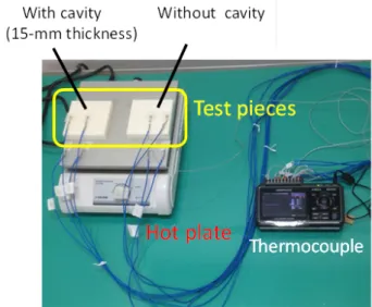
In this study, we present three dimensional shape identification of cavity in structure based on the finite element and adjoint variable methods using the temperature history on specimen surface. It is known that if there is a cavity in the target structure, existence of cavity can be confirmed by the thermal testing method (See Figs. 1, 2 and 3)[1]. However, size or shape of the cavity can’t be numerically evaluated based on the heat image on surface of target structure.

Therefore, in this study, we measured time history of temperature on test piece, i.e., resin structure with cavity made by 3D printer, and carried out the shape identification of cavity based on the adjoint variable and finite element

methods[2][3].

Figure 1. Experimental apparatus.

2. Formulations based on the adjoint variable and the finite element methods The heat transfer equation shown in Eq.(1) is employed as the basic equation.

ρc ϕ ˙ − κϕ

= 0 (1)

where ρ, c, ϕ and κ indicate the dencity, the specific heat, the temperature and the thermal conductivity. Here, the performance function is defined as shown in Eq.(2) to identify the cavity shape[4].

J = 1 2

∫

Γobs

∫

R (ϕ − ϕ

)

dt dΩ (2)

24 26 28 30 32 34 36 38

0 200 400 600 800 1000 1200

Temperature (deg C)

Time (s)

With cavity Without cavity

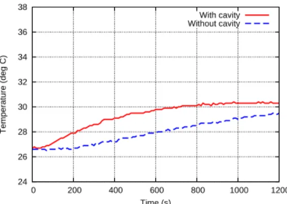
Figure 2. Time history of temperature on test piece at center point of upper surface.

Figure 3. Heat image on surface of test piece.

where Γ

, t

, R and ϕ

denote the observation boundaty, the terminal time (Total time), the weighting constant and the observed temperature. The problem is to find the cavity shape such that the computed temperature is close to the target temperature under the condition of the basic eqution, Eq.(1). To do that, the Lagrange multiplier method is introduced[5][6], and the performance function is extened as shown in Eq.(3).

J

= J +

∫

Ω

∫

t₀

λ (

ρc ϕ ˙ − κϕ

)

dt dΩ (3)

where λ indicates the Lagrange multiplier. To obtaine the stationary condition of the Lagrange function J

, the fist variation of the Lagrange function is calculated. Consequently, the adjoint eqaution that is the equation for the Lagrange multiplier is obtained as shwon in Eq.(4).

− ρc λ ˙ − κλ

+ R (ϕ − ϕ

) = 0 (4) The terminal condition and the boundary condition for the Lagrange multiplier is given to solve the adjoint equation.

Those conditions are obtained from the result of the first variation of the Lagrange function.

3. Numerical experiment for shape identification 3.1. Computational condition

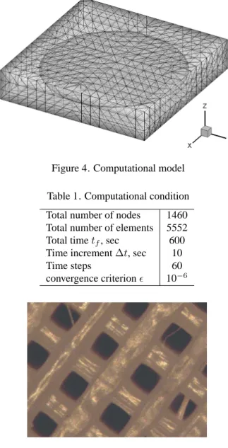
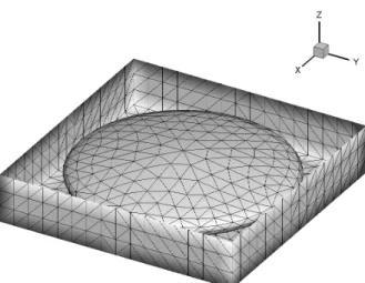
The finite element model of the test piece is shown in Figure 4. The model is composed four-node tetrahedral element.

Total number of nodes are 1460, and total number of elements are 5552. Thermal property and computational condition (See Table 1) are identical with numerical simulation shown in previous chapter. The computational conditions are referred to experiment and given as Table 1. Thermal properties for the test piece is given as shown in Table 2

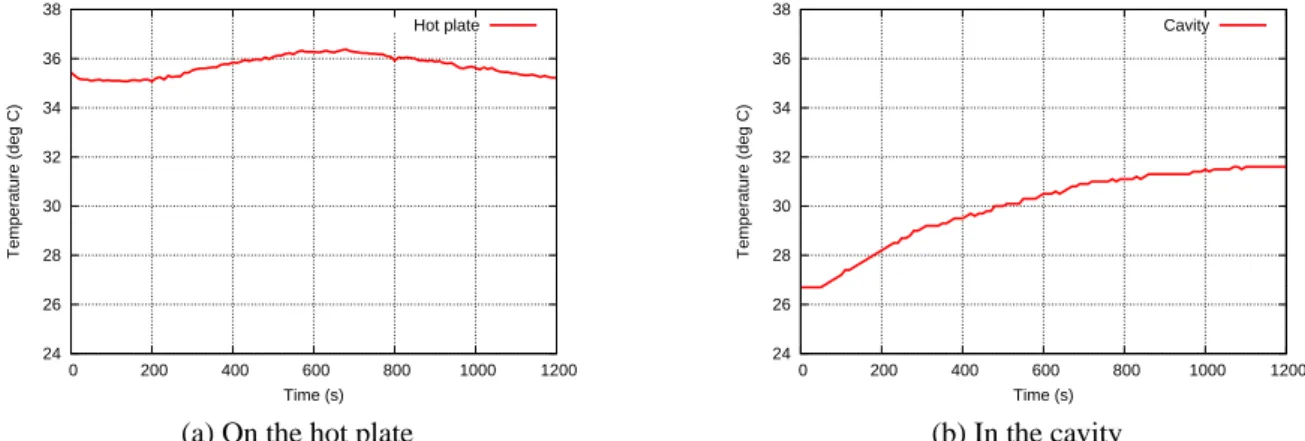
considering the thing which the ABS resin is not filled enough shown in Figure 5. The observational data at Point A in the previous experiment is employed as observed temperature. In addition, the time history of temperature on the hot plate and temperature within the cavity as boundary conditions are shown in Figure 6(a) and (b).

3.2. Computational results

Figure 7 shows estimated shape of the cavity and Figure 8(a) shows variation of normalized performance function per

iteration number. Final iteration number is 18, performance function is about 0.55 when converting initial performance

function into 1. However surface of the cavity becomes undulation, targeted shape as 15mm thickness cavity cannot be

obtained. Additionally estimated volume of the resin region doesn’t reach similar form to target value (See Figure 8(b))

Figure 4. Computational model Table 1. Computational condition Total number of nodes 1460 Total number of elements 5552 Total time t

, sec 600 Time increment ∆t, sec 10

Time steps 60

convergence criterion ϵ 10

Figure 5. Cross-section of test piece Table 2. Computational condition

Density ρ Specific heat c Thermal conductivity κ Heat transfer coefficient Outside surface h

Cavity h

kg/m

J/(kg

C) W/(m

C) W/(m

C) W/(m

C)

ABS 750 1386 0.1354 10.0 7.0

3.3. Gaussian filter

The smoothing process for gradient vector is introduced to modify the oscillation of the gradient vector with respect to coordinate on cavity surface. For the smoothing method, Gaussian filter[7] is employed. Looking at the surface of the cavity as two-dimensional surface, the gradient vector is smoothed. Gaussian filter is a kind of the smoothing filter for the field of graphics. In smoothing method with Gaussian filter input of weighting parameter, value of the target nodes is determined by value of all nodes on the same plane. And the Gaussian filter has the advantage that the extent of the smoothing process is adjustable with the parameter σ. The weighting parameter in Gaussian filter[8] is defined as following equation:

G(x, y) = 1

2πσ

e

2

2σ2

(5)

where x and y is the distance of x-axial distance and y-axial distance between the target node and referenced node. The

weighting parameter becomes large value if the distance is short. The parameter σ which is comparable to the variance in

24 26 28 30 32 34 36 38

0 200 400 600 800 1000 1200

Temperature (deg C)

Time (s)

Hot plate

(a) On the hot plate

24 26 28 30 32 34 36 38

0 200 400 600 800 1000 1200

Temperature (deg C)

Time (s)

Cavity

(b) In the cavity Figure 6. Time history of temperature of resin surface (1)

Figure 7. The shape of cavity in final iteration

0 0.1 0.2 0.3 0.4 0.5 0.6 0.7 0.8 0.9 1

0 5 10 15 20

Normalized performance function

Number of iterations Performance function

(a) Performance function

130000 135000 140000 145000 150000

0 5 10 15 20

Volume(mm3)

Number of iterations Estimated shape

Target value

(b) Volume of the resin region Figure 8. Computational result(1)

Gaussian distribution determines flattening of the distribution. In addition, as the summation of the weighting parameter for the target node becomes 1, we multiply the weighting parameter by the summation. The weighting parameter for node m to node n is shown in following equation:

G

=

1 2πσ²

e

(m)−x(n) )2+(y(m)−y(n) )2 2σ2

∑

1 2πσ

e

(m)−x(n) )2+(y(m)−y(n) )2 2σ2

(6)

where cx means the number of nodes on the surface, x

and y

mean x-coordinate and y-coordinate of the node i.

On the gradient vector {

∂J^∗

∂x^(m)_i

}

, smoothed gradient vector {

∂J^∗

∂x^(m)_i

′

}

is computed. The calculating formula is represented as following matrix form.

 

 

 

 

 

 

 



∂J^∗

∂x⁽¹⁾_i

′

∂J^∗

∂x⁽²⁾_i

′

.. .

∂J^∗

∂x^(cx)_i

′

 

 

 

 

 

 

 



=



 

 

G

G

· · · G

G

G

· · · G

.. . .. . . . . .. . G

G

· · · G



 

 

 

 

 



 

 

 

∂J^∗

∂x⁽¹⁾_i

∂J^∗

∂x⁽²⁾_i

.. .

∂J^∗

∂x^(cx)_i

 

 

 



 

 

 

(7)

3.4. Shape estimation with Gaussian filter

In the Gaussian filter, the parameter σ is given as 20, and the shape estimation analysis is carried out. The estimated shape of the cavity is shown in Figure 9. The surface of the cavity is smoother than the result without smoothing process in previous section. As the variation of performance function, in the case using Gaussian filter, number of iteration is larger and performance function is lower (See Figure 10(a)). In addition, it is found that the difference of the computed volume of the resin region at each iteration and the target volume decreases (See Figure 10(b)). It is confirmed that the temperature comes closer to observed value by applying smoothing process.

Figure 9. The shape of cavity in final iteration

0 0.1 0.2 0.3 0.4 0.5 0.6 0.7 0.8 0.9 1

0 10 20 30 40 50 60

Normalized performance function

Number of iterations Without smoothing

With smoothing

(a) Performance function

130000 135000 140000 145000 150000

10 20 30 40 50 60

Volume(mm3)

Number of iterations Without smoothing

With smoothing Target value

(b) Volume of the resin region Figure 10. Computational result(2)

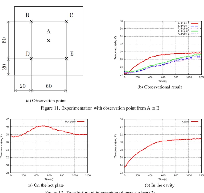
3.5. The effect of observation point

It is found that identified shape is not good agreement with the target shape, even if the smoothing method is applied. It

appears that the computational accuracy increases with increasing the number of observation points. The experimentation

using the test piece with a 15-mm cavity was carried out newly. A lot of 5 observation points including Point A in

previous observation are shown in Figure 11(a). Then observational results are shown in Figure 11(b) and Figure 12.

(a) Observation point

24 26 28 30 32 34 36 38

0 200 400 600 800 1000 1200

Temperature(deg C)

Time(s)

At Point A At Point B At Point C At Point D At Point E

(b) Observational result

Figure 11. Experimentation with observation point from A to E

28 30 32 34 36 38 40 42

0 200 400 600 800 1000 1200

Temperature(deg C)

Time(s)

Hot plate

(a) On the hot plate

22 24 26 28 30 32 34 36

0 200 400 600 800 1000 1200

Temperature(deg C)

Time(s)

Cavity

(b) In the cavity Figure 12. Time history of temperature of resin surface (2)

3.6. Shape identification with multiple observation points

The shape identification analysis is carried out under the three conditions shown below.

Applying time history of temperature at 1. 1 observation points (Point A)

2. 3 observation points (Point A, Point B and Point E) 3. 5 observation points

The value of the performance function is calculated by using the data at point A in three computational conditions. The final shape of the cavity in the computational condition (3) is shown in Figure 13. From this result, it is confirmed that there is no big difference in each case. In addition, variations of performance function and the volume of resin are shown in Figures 14(a) and (b). Consequently, it is seen that the volume in case of five observation points is close to the target volume. Figure 15 shows comparison of the identified shape and target shape. It is found that the position of the identified shape is upper than that of the target shape.

4. Conclusions

In this study, the shape identification of the cavity in three dimensions are carried out using the data of the observed

temperature on test piece surface. As for the computational method, the adjoint variable and the finite element methods

are employed. In addition, the Gaussian filter is applied to obtain the smoothed gradient with respect to the coordinates

on cavity surface. Consequently, it is found that if the smoothing technique is employed, and the cavity shape is

appropriately identified comparing to the result without the smoothing technique.

Figure 13. The shape of the cavity at the final iteration(3)

0 0.1 0.2 0.3 0.4 0.5 0.6 0.7 0.8 0.9 1

0 10 20 30 40 50 60

Normalized performance function

Number of iterations 1 observation point 3 observation point 5 observation point

(a) Performance function

130000 135000 140000 145000 150000

0 10 20 30 40 50 60

Volume(mm3)

Number of iterations 1 observation point 3 observation point 5 observation point Target value

(b) Volume of the resin region Figure 14. Computational result(2)

Figure 15. Comparison of identified shaoe with target shape Acknowledgement

This work was supported by ”Program for High Reliable Materials Design and Manufacturing in Nagaona University of Technology”.

References

1. V. Dattoma, R. Marcuccio, C. Pappalettere and G.M. Smith, Thermographic investigation of sandwich structure made of composite material, NDT & E Int., Vol. 34(8), Dec., pp. 515-520, 2001.

2. T. Kurahashi and H. Oshita, Evaluation of 3D Reinforcement Corrosion Shape in Concrete Based on Observed Temperature on Concrete Surface, IJCS, Vol. 4(4), pp. 340-351, 2010.

3. T. Kurahashi and H. Oshita, Shape Determination of 3-D Reinforcement corrosion in Concrete Based on Observed

Temperature on Concrete Surface, Computers and Concrete, Vol. 7(1), pp. 63-81, 2010.

4. H. Oshita, H. Horie, S. Nagasaka, O. Taniguchi, and S. Yoshikawa, Nondestructive evaluation of corrosion in reinforced concrete by thermal behavior on concrete due to electromagnetic heating, J. of JSCE-E, Vol. 65(1), pp. 76-92, 2009.

5. T. Kurahashi and M. Kawahara, Examinations for thermal condition of Lagrange multiplier for heat transfer control problems, IJNME, Vol. 73, pp. 982-1009, 2008.

6. T. Kurahashi, Examination for adjoint boundary conditions in initial water elevation estimation problems, IJNMF, Vol. 63, pp. 1270-1295, 2010.

7. S. Wang, W. Li, Y. Wang, Y. Jiang, S. Jiang and R. Zhao, An improved Difference of Gaussian Filter in Face Recognition, JMM, Vol. 7(6), pp. 429-433, 2012.

8. H. Ishiwata, H. Kubota and Y. Shima, Experimental study on Gaussian filter in restoration of error diffused character

images, IPSJ, Vol. 51(2006-CVIM-154), pp. 23-28, 2006.