Instructions for use
A uthor(s ) HOR A ,A kihito
C itation Hokkaido University Preprint S eries in Mathematics, 1056: 1-28
Is s ue D ate 2014-5-26
D O I 10.14943/84200
D oc UR L http://hdl.handle.net/2115/69860
T ype bulletin (article)
F ile Information pre1056.pdf
PLANCHEREL ENSEMBLE OF YOUNG DIAGRAMS AND FREE PROBABILITY
AKIHITO HORA
Abstract. Concentration phenomena in statistical ensembles of Young diagrams have been investigated as static models first for the Plancherel ensemble by Vershik–Kerov and Logan–Shepp in 1970s and later for some other group-theoretical ensembles by Biane. On the other hand, a dynamical model of concentration for Young diagrams, which is not directly connected with group representations, was shown by Funaki– Sasada in the framework of hydrodynamic limit. Our aim here is to dis-cuss a dynamical model of concentration for Young diagrams in group-theoretical ensembles. We especially feature Biane’s approximate factor-ization property of ensembles as an origin to give rise to concentration. Starting from an initial ensemble yielding concentration and a micro-scopic dynamics keeping the Plancherel measure invariant, we derive an evolution of rescaled shapes of Young diagrams through hydrodynamic limit. The resulting evolution along macroscopic time is described in terms of the notions of Voiculescu’s free probability theory such as free compression and free convolution of Kerov transition measures.
1. Introduction
The set of Young diagrams of sizen, which is denoted byYn, parametrizes
all the equivalence classes of irreducible representations of the symmetric groupSn. The Plancherel measure M(n)
Pl is a fundamental probability
mea-sure onYn, which is defined by
(1.1) M(n)
Pl (λ) =
(dimλ)2
n! , λ∈Yn,
where dimλ denotes the dimension of an irreducible representation of Sn
labeled by λ ∈ Yn. The probability space (Yn,M(n)
Pl ) is often called the
Plancherel ensemble of Young diagrams of sizen. It is known that a Young diagram chosen out of the Plancherel ensemble at random, strictly speaking according to the probability designed by M(n)
Pl , should always look like a
special shape. This is the famous concentration phenomenon to the limit
2010 Mathematics Subject Classification. Primary 82C41 ; Secondary 20C30, 46L54, 60J27.
Key words and phrases. hydrodynamic limit, Young diagram, symmetric group, free probability, Markov chain, Plancherel measure, Kerov polynomial.
shape discovered by Logan–Shepp[14] and Vershik–Kerov[17]. A more pre-cise statement is formulated as a weak law of large numbers as follows. Identifying a Young diagram λ ∈ Yn with its profile as defined in
Subsec-tion2.1(see Figure1), we consider the rescaled function by 1/√n:
(1.2) λ√n(x) = √1
nλ( √
nx), x∈R.
Set
(1.3) Ω(x) =
{ 2
π(xarcsinx2 +
√
4−x2), |x|≦2,
|x| |x|>2.
Then, for anyϵ >0, we have
(1.4) lim
n→∞M (n) Pl
({
λ∈Yn sup
x∈R|
λ√n(x)−Ω(x)|≧ϵ})= 0.
The Plancherel measure can be lifted to the probabilityMPl on the spaceT
consisting of the paths of Young diagrams
(1.5) t=(t(0) =∅↗t(1) =□↗t(2)↗ · · · ↗t(n)↗ · · ·), t(n)∈Yn
so that it is the nth marginal distribution as
(1.6) M(n)
Pl (λ) =MPl({t∈T|t(n) =λ}), λ∈Yn.
Then we can show almost sure convergence to the limit shape Ω as a
strong law of large numbers. These kinds of concentration are observed in other ensembles than the Plancherel one. In [1] and [2], Biane pointed out the property of “approximate factorization” for states of group algebra
C[Sn] induced by probabilities on Yn and gave many interesting examples
of these concentration phenomena. Approximate factorization property is interpreted as ergodicity in a certain weak sense. The limit shape in the Plancherel ensemble simply means the 1-point function of the system. A thorough treatment including higher correlation functions was developed by Borodin–Okounkov–Olshanski[4].
totality of Young diagrams of all sizes allows variation of the number of boxes. The main theorem of this paper is stated in the canonical ensemble setting where we consider a Markov chain on Yn and then take a limit of n → ∞. When we discuss the Plancherel ensemble in the grand canoni-cal manner, it seems natural to consider the probability on Y = ⊔∞
n=0Yn
through poissonization ofM(n)
Pl ’s. In Section4, we formulate this model and
state some aspects which we meet with in computing its hydrodynamic limit. The framework of the hydrodynamic limit in this paper is as follows. Recall that, if the microscopic Plancherel ensemble is zoomed out under scaling limit by 1/√nas (1.2), one observesΩof (1.3) macroscopically. We consider a continuous time Markov chain (Xs(n))s≧0 on the state space Yn
which keeps the Plancherel measure M(n)
Pl invariant. Then, starting from
the initial stateM(n)
Pl , the macroscopic shape remainsΩas time goes by. As
an initial state on Yn let us now take a probability M(n)
0 under which the
ensemble yields concentration as n→ ∞. After 1/√n-scaling limit of (1.2) with respect to M(n)
0 , a certain macroscopic shape ω0 is observed. When
we drive the same Markov chain as above from the initial state M(n)
0 , it is
expected that the distribution M(n)s onYn at time s will tend toM(n)
Pl ass
goes by. Then, seen from the macroscopic point of view, an evolution from
ω0 toΩ should be observed. Speaking the scale more precisely, we assume
that the microscopic ensemble (Yn,M(n)
0 ) appears if the macroscopic initial
shapeω0 is zoomed in by rescale of√nmultiple. Given a macroscopic time
t > 0, we consider the situation of the ensemble after microscopically long time s = tn and, observing it by the rescale of 1/√n, see a macroscopic shapeωtat timet. Note that the scale of time vs space is the diffusive one.
Our aim is to prove this concentration toωt at each time tand to describe
ωt as explicitly as possible as a function oft. Since we have convergence to
the Plancherel measure as s → ∞ in the microscopic situation, ωt should
converge to the limit shapeΩ ast→ ∞.
Let us proceed to state our main theorem which realizes the above frame-work. In order to take a Markov chain on Yn which keeps M(n)
Pl invariant,
we consider (a special case of) the up and down transition probabilities used in [5]. For two Young diagramsλandµ, whose sizes satisfying|λ|+ 1 =|µ|, we use the notation of λ↗ µ if µ is formed by adding one box to λ. For
λ∈Yn (n∈N), set
(1.7)
Pλ,µ↑ =
{ dimµ
(n+1) dimλ, λ↗µ(∈Yn+1),
0, otherwise, P
↓ λ,µ=
{dimµ
dimλ, µ(∈Yn−1)↗λ,
0, otherwise.
The branching rules of induction and restriction
IndSn+1 Sn λ∼=
⊕
µ∈Yn+1:λ↗µ
µ, ResSn Sn−1λ∼=
⊕
µ∈Yn−1:µ↗λ
yield thatP↑ and P↓ satisfy
∑
µ∈Yn+1
Pλ,µ↑ = 1, ∑
µ∈Yn−1
Pλ,µ↓ = 1.
Hence, setting P(n) =P↑P↓, namely
(1.8) Pλ,µ(n)= ∑
ν∈Yn+1
Pλ,ν↑ Pν,µ↓ , λ, µ∈Yn,
we have P(n) to be a stochastic matrix of degree |Y n|.
Lemma 1.1. M(n)
Pl of(1.1)is symmetric with respect toP(n)of(1.8), namely
we have
(1.9) M(n)
Pl (λ)P (n) λ,µ =M
(n) Pl (µ)P
(n)
µ,λ, λ, µ∈Yn.
Hence a Markov chain on Yn with the transition probability matrix P(n) keeps M(n)
Pl invariant.
Proof. We see from (1.8) and (1.7)
Pλ,µ(n)= ∑
ν∈Yn+1:λ↗ν,µ↗ν
dimµ
(n+ 1) dimλ.
If λ, µ ∈ Yn are distinct, then Young diagram ν ∈ Yn+1 satisfying both
λ ↗ ν and µ ↗ ν can exist at most one, which could be ν = λ∨µ (=
set-theoretical union of the boxes). The number of Young diagrams ν ∈ Yn+1 satisfying λ↗ ν agrees with the number of valleys of λ(see (2.1) in
Section2). We thus obtain
(1.10) Pλ,µ(n)=
|{valleys ofλ}|
n+1 , λ=µ, dimµ
(n+1) dimλ, λ∨µ∈Yn+1,
0, otherwise
forλ, µ∈Yn. (1.9) follows from (1.1) and (1.10). □
Let us consider a continuous time Markov chain (Xs(n))s≧0 with the
tran-sition matrix P(n) on the state spaceYn. M(n) denotes the induced
proba-bility on the set of functions (= paths) from [0,∞) to Yn. M(n)
0 being the
initial distribution on Yn, the distribution M(n)(Xs(n) = · ) at time s is
given by
(1.11) M(n)(Xs(n)=µ) = ∑
λ∈Yn M(n)
0 (λ)(es(P
(n)−I)
)λ,µ, µ∈Yn.
Identifying a Young diagram with its profile, put it into the space D
ω∈Dis by definition a functionR−→Rsatisfying the following conditions:
|ω(x)−ω(y)|≦|x−y|, x, y∈R,
(1.12)
ω(x) =|x| if|x|is large enough.
(1.13)
mω denotes the transition measure of ω ∈ D (see (2.2) in Subsection2.1).
The transition measure ofΩ in (1.3) is the standard semi-circle distribution such that
(1.14) mΩ(dx) = 1
2π
√
4−x21
[−2,2](x)dx.
For a probability on R, its kth moment and free cumulant are denoted by Mk(·) and Rk( ·) respectively, k∈N (see Subsection2.2). A decisive fact
is that the free cumulant sequence of (1.14) is
R1(mΩ) = 0, R2(mΩ) = 1,
(1.15)
R3(mΩ) =R4(mΩ) =R5(mΩ) =· · ·= 0.
The ensembles admitting approximate factorization property cover a wide range of known examples for concentration phenomena ([2]). We formulate the relevant conditions and resulting concentration as follows (partly re-calling [8], [9]). Given a probability M on Yn, we have a positive-definite
normalized central function on Sn by
(1.16) f(x) = ∑
λ∈Yn
M(λ) ˜χλ(x), x∈Sn.
Here χλ is the irreducible character of S
n labeled by λ, and we set ˜χλ =
χλ/dimλ. The mapM 7→ f of (1.16) is an affine bijection from the set of
probabilities on Yn onto
(1.17){
f :Sn−→Cpositive-definite, f(e) = 1, f(x−1yx) =f(y) (x, y∈Sn)}.
Moreover, f in (1.17) is uniquely extended to a tracial state of C[Sn] by
linearity. If f is a central function on Sn and σ is a Young diagram with
|σ| ≦ n, the value of f at an element of cycle type σ inSn is denoted by
f(σ,1n−|σ|). Note that σ can contain one-box rows in this notation.
Definition 1.2. Given ensemble {(Yn,M(n))}n∈N, let f(n) be the
corre-sponding tracial state of C[Sn] determined by (1.16). We refer to the
fol-lowing set of conditions as Condition (AF).
•(approximate factorization property) For any p ∈N and anyk1,· · · , kp ∈ {2,3,· · · },
(1.18)
f(n)
((k1)⊔···⊔(kp),1n−(k1+···+kp))−f
(n)
(k1,1n−k1)· · ·f
(n)
(kp,1n−kp)=o
(
n−(k1−1)+···2+(kp−1))
•(asymptotic cycle mean) There exista >0 and a real sequence{r3, r4,· · · }
such that, for any k∈ {2,3,· · · },
lim
n→∞n
k−1 2 f(n)
(k,1n−k)=rk+1,
(1.19)
|rk+1|≦ak+1.
(1.20)
□
The meaning of growth order nk−21 for the k-cycle value appearing in
(1.18) and (1.19) of Condition (AF) may be unclear at a glance. One will be convinced by knowing the form of Kerov polynomials that this growth order fits with our rescale of (1.2). See the approximate computation (2.17) in Subsection2.3.
Theorem 1.3. Let ensemble {(Yn,M(n))}n∈N satisfy Condition (AF) of Definition1.2. Then, there exists ω∈Dsuch that
(1.21) lim
n→∞M
(n)({λ∈Y n
sup
x∈R|
λ√n(x)−ω(x)|≧ϵ})= 0
for any ϵ >0.
We call the continuous diagram ω the macroscopic shape forM(n).
This concentration result is due to Biane ([1], [2]). Proof of Theorem1.3 is reconstructed in Section3 for the use of proving the main theorem. A stronger fact than (1.21) is shown in (3.8) and (3.10). As typical examples of ensembles satisfying Condition (AF), we mention later in AppendixA bal-anced irreducible characters and Thoma ensembles. Something like indepen-dence is suggested by (1.18) for indicator functions with disjoint supports. It will be also clarified there that approximate factorization property can be regarded as a certain weak ergodicity of the ensemble.
Here is our main theorem. Free convolution of two probabilities µ and
ν on R is denoted by µ⊞ν. For a probability µ on R and c ∈ (0,1], µc
denotes the probability on R obtained as free compression by a projection
of expectation c(see Subsection2.2).
Theorem 1.4. For the Markov chain (Xs(n))s≧0 of (1.11), assume that
ini-tial ensemble{(Yn,M(n)
0 )}n∈Nsatisfies Condition (AF) of Definition1.2. For any (macroscopic time)t≧0, consider the distribution of the Markov chain at s=tn:
(1.22) M(n)t (λ) =M(n)(Xtn(n)=λ), λ∈Yn.
Then,{(Yn,M(n)t )}n∈N satisfies Condition (AF) for anyt≧0. There exists a function t∈[0,∞)7−→ωt∈D such that, for any t≧0 and any ϵ >0,
(1.23) lim
n→∞M (n) t
({
λ∈Yn sup
x∈R|
λ√n(x)−ωt(x)|≧ϵ})= 0.
Here the macroscopic shape ωt ∈ D at time t is characterized through its
transition measure mω
free convolution:
(1.24) mω
t = (mω0)e−t ⊞(mΩ)1−e−t, t >0.
Remark1.5. In terms of a free cumulant sequence1, (1.24) is translated into
R1(mωt) = 0, R2(mωt) = 1,
(1.25)
Rk(mωt) =Rk(mω0)e−
(k−1)t, k≧3
(see (2.10) and (2.8) in Section2 for the free cumulants obtained by free compression and free convolution). Since we have for anyk∈N
(1.26) lim
t→∞Rk( mω
t) =Rk(mΩ)
by (1.25),ωt converges toΩ inDast→ ∞ in a macroscopic point of view.
Remark 1.6. If we adopt P↓P↑ instead of P↑P↓ as the transition matrix of a Markov chain on Yn governing the microscopic dynamics, we still have
invariance of M(n)
Pl and the same result for hydrodynamic limit. See
Re-mark3.5.
In [7] and most results on hydrodynamic limit in other models also, a fundamental task is to describe the evolution along macroscopic time by specifying a (non-linear) partial differential equation forωtobtained through
the scaling limit. In the contexts of this paper, as may be seen from the strategy of the proof of Theorem1.4 stated in the next paragraph, the shape of an element ofDcan be efficiently analyzed by the free cumulant sequence
of the transition measure. The correspondence between
ω∈D ←→ mω ←→ {Rk(mω)}k∈N
will be explained in Subsections 2.1 and 2.2 . As for a partial differential equation for the evolution, we derive the one for the Stieltjes transform of
mω
t:
(1.27) G(t, z) =
∫
R
1
z−xmωt(dx), z∈C
+
in Proposition3.3.
Let us note brief ideas for the proofs of Theorem1.3 and Theorem1.4, whose details are written in Section3. Since the Plancherel ensemble comes from representations of symmetric groups, it is congenial to group characters in computation. Our basic trick is as follows. In computing expectations, devise to replace free cumulant Rk+1(mλ) of the transition measure mλ of
λ∈ Yn by the (suitably normalized) irreducible character value at k-cycle
of Sn corresponding toλ. These procedures are justified by analysis of the
Kerov–Olshanski algebra consisting of polynomial functions of coordinates of Young diagrams as well as a (rough) application of the so-called Kerov poly-nomial. We review these notions in Subsection2.3. Such replacement being justified, the proof of Theorem1.4 will proceed by using induction/restriction
of irreducible characters and similar devices for proving concentration to the limit shapeΩ.
After Introduction, the subsequent sections are organized as follows. Sec-tion2 is devoted to reviewing necessary notions and properties. Introduced are the profile of a Young diagram, its transition measure, several notions in Voiculescu’s free probability theory and so on. Then we give explanations on structure of the Kerov–Olshanski algebra and the Kerov polynomials. The proofs of Theorem1.3 and Theorem1.4 are given in Section3 along the strategy stated above. In Section4, we consider the poissonized Plancherel ensemble in which the microscopic dynamics allows variation of sizes of Young diagrams and discuss a setting of the grand canonical ensemble for hydrodynamic limit. Finally, we supplement comments about some results on approximate factorization property for a state of the group algebra of a symmetric group in AppendixA.
2. Preliminaries
2.1. Young diagram, continuous diagram and transition measure.
A Young diagram is presented by λ= (λ1 ≧ λ2 ≧ · · · ≧ λl(λ) > 0) where
l(λ) denotes the number of rows inλor by λ= (1m1(λ)2m2(λ)· · ·jmj(λ)· · ·)
wheremj(λ) denotes the number of rows of length j inλ. In this paper we
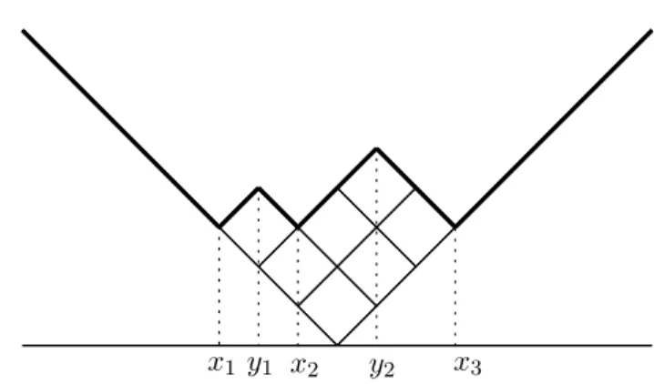
mainly display a Young diagram by loading the region y > |x| of the xy -plane with squares (= boxes) of edge length√2 as Figure1. The piecewise linear graph presented by bold lines in Figure1 is called the profile of a Young diagram. A Young diagram identified with its profile is regarded as a continuous diagram defined by (1.12) and (1.13). Setting D0 = {λ ∈ D|λis piecewise linear, λ′(x) = ±1}, we have Y ⊂ D0 ⊂ D. We encode λ∈D0 by using the x-coordinates of the valleys and peaks ofλ
(2.1) x1 < y1 < x2 < y2 <· · ·< xr−1 < yr−1 < xr
x1 y1 x2 y2 x3
as Figure1. Conversely, interlacingxi’s and yi’s as (2.1) are the coordinates
of some λ∈D0 if and only if they satisfy
r ∑
i=1
xi− r−1 ∑
i=1
yi= 0.
An atomic probabilitymλ on R is uniquely assigned to anyλ= (x1 < y1< · · ·< yr−1 < xr)∈D0 by
(2.2) (z−y1)· · ·(z−yr−1) (z−x1)· · ·(z−xr)
=
∫
R
1
z−xmλ(dx), z∈C\R.
Clearly, suppmλ coincides with{x1,· · · , xr}. mλ is called the (Kerov)
tran-sition measure of λ. On the other hand, the Rayleigh measure ofλ∈D0 is
defined by
(2.3) τλ=
r ∑
i=1
δxi−
r−1 ∑
i=1
δyi
as a signed measure on R with total measure 1. The moment sequences {Mn(mλ)}n=0,1,2,··· and {Mn(τλ)}n=0,1,2,··· forλ∈D0 are related by
(2.4)
∞ ∑
n=0
Mn(mλ)
zn = exp
(∑∞
k=1
Mk(τλ)
kzk )
, z∈C, |z| ≫1.
As a consequence of (2.4), we see that {Mn(mλ)} and {Mn(τλ)} are
ex-pressed as polynomials of each other. The transition measure mω can be
defined for any continuous diagram ω ∈ D also through a limiting
proce-dure. A convenient way is that, taking a uniformly approximate sequence
{λ(k)}
k∈N ⊂ D0 for a given ω ∈ D and recognizing that {Mn(mλ(k))}k∈N
forms a Cauchy sequence for any n ∈ N by the above mentioned
polyno-mial relations, we apply an easy moment problem for a compactly supported probability onR. Then, (2.4) is extended to
(2.5)
∫
R
1
z−xmω(dx) =
1
zexp
{∫
R
1
x−z
(ω(x)− |x|
2
)′
dx}, z∈C\R
for ω ∈ D. Conversely, given a probability µ on R with compact support
and mean 0, there corresponds a unique ω ∈ D such that µ= mω, though
Rayleigh measure τω does not necessarily exist. In this case, we mention a
Rayleigh function F : R −→ [0,1], which satisfies by definition F(x) = 0
on (−∞, a] and F(x) = 1 on [b,∞) for some a, b ∈ R and coincides with
the distribution function of the Rayleigh measure if it exists. The relation corresponding to (2.5) betweenµ,F andω is given by
∫
R
1
z−xµ(dx) =
1 zexp { − ∫ 0 −∞
F(x)
z−xdx+
∫ ∞
0
1−F(x)
z−x dx
}
,
(2.6)
ω(u) =
∫ u
−∞
F(x)dx+
∫ ∞
u
(1−F(x))dx.
In this paper, we treat only the case where suppµ is compact. Including consideration of probabilities with non-compact supports and certain mo-ment conditions, a thorough treatmo-ment of interplay between µ, F and ω is given in [12]. The mapF 7→µis called the Markov transform. Let us refer to the topology onDdefined by the family of semi-distances
{
dk(ω1, ω2) =|Mk(mω1)−Mk(mω2)|(ω1, ω2∈D)
} k∈N.
as the moment topology on D. We see the following facts about topologies
on Dfrom the definition ofD and (2.5).
Lemma 2.1. (1) The pointwise and uniform convergence topologies on D coincide.
(2) Restricted on {ω ∈D|ω(x) =|x|for |x|≧a} for a >0, the uniform convergence and moment topologies coincide.
(3) The moment topology is stronger than the uniform convergence one onD.
Proof. (1) directly follows from the conditions (1.12) and (1.13) to defineD.
(2) and (3) are shown by using (2.5). □
2.2. Free probability theory. Let us recall several notions in free prob-ability theory due to Voiculescu. See [15] for details. Here we mainly pick up combinatorial aspects only for one-dimensional distributions. Consider a
C∗-probability space (A, ϕ) consisting of a unital C∗-algebra A and a state
ϕofA. Letµ, ν be the distributions of self-adjointa, b∈ Arespectively. Ifa
andbare free, the distribution ofa+bis denoted byµ⊞νand called the (ad-ditive) free convolution ofµandν. Given compactly supported probabilities
µ, ν on R,µ⊞ν is uniquely determined and compactly supported. In terms of free cumulants of probabilities onR, the free convolution is characterized
by
(2.8) Rk(µ⊞ν) =Rk(µ) +Rk(ν), k∈N.
Here Rk(µ) denotes the kth free cumulant of µ, which is defined (from a
combinatorial viewpoint) by the following cumulant-moment formula (2.9). NC(n) denoting the set of non-crossing partitions of {1,2,· · ·, n}, extend subscripts of cumulants (and moments also) to partitionπ = (v1,· · · , vl)∈
NC(n) by setting
Rπ(µ) =R|v1|(µ)· · ·R|vl|(µ)
multiplicatively (where |vi| denotes the cardinality of block vi). Then, we
have
(2.9) Mn(µ) =
∑
π∈NC(n)
Rπ(µ), n∈N.
The M¨obius function of the poset NC(n) enables us to write an inversion formula of (2.9), which expresses Rn(µ) explicitly in terms ofMk(µ)’s.
Ifq∈ Ais a projection (q2 =q=q∗) such that the expectationϕ(q)̸= 0,
setting B = qAq and c = ϕ(q), we have a C∗-probability space (B,1cϕ
Moreover, if self-adjoint a ∈ A and q are free, then the distribution of qaq
with respect to 1cϕ
B is called the free compression of the distribution µ of
aand denoted byµc. Given a compactly supported probabilityµon Rand
c∈(0,1], the free compression µc of µ is uniquely determined. In terms of
free cumulants, the free compression is characterized by
(2.10) Rk(µc) =ck−1Rk(µ) (=
1
cRk(µ(
1
c·))
)
, k∈N.
For a compactly supported probabilityµ onR, set
(2.11) Kµ(ζ) =
1
ζ +
∞ ∑
k=0
Rk+1(µ)ζk, ζ ∈C.
The Taylor series part of (2.11) is Voiculescu’s R-transform of µ. Kµ of
(2.11) and the Stieltjes transform
Gµ(z) = ∫
R
1
z−xµ(dx), z∈C
of µ are inverse functions of each other in appropriate domains such that
|ζ| ≪1←→ |z| ≫1.
2.3. Kerov–Olshanski algebra. An algebra of polynomial functions in the coordinates encoding Young diagrams was introduced in [13] and plays an important role in asymptotic representation theory of symmetric groups. It is essential to compute the transition coefficients between several generat-ing systems of the algebra as explicitly as possible. Substantial contributions in this direction were given in [11]. It is natural to define this algebra by introducing as generators the power sums
pn(λ) = ∑
i (
ani + (−1)n−1bni)
which are supersymmetric with respect to the Frobenius coordinates (ai, bi)
of Young diagrams. In this paper, however, since we mainly utilize the
x-coordinates of the valleys and peaks (2.1) as coordinates of Young dia-grams, we pick up defining generators in terms of these coordinates from the beginning.
For λ= (x1 < y1 < · · · < yr−1 < xr) ∈ Y, consider the nth moment of
the Rayleigh measureτλ (2.3) of λ:
(2.12) Mn(τλ) =
r ∑
i=1
xni −
r−1 ∑
i=1
yni, n∈N.
Mn(τλ)’s for n≧2 are algebraically independent (overR). Actually, (
M2(τλ)M3(τλ) · · ·)=(2p1(λ) 3p2(λ) · · ·)A
holds for an upper triangular matrix A = (aij) with aii = 1, aij ≧ 0. Let
us call the algebra Agenerated by{1, Mn(τλ)|n∈ {2,3,· · · }} (over R) the
declareMn(τλ) to be annth homogeneous element ofA. This gives rise to a
filtration inA. Then, the top degree off ∈Ais denoted by wt(f). The
sym-bol wt comes from “weight” (see [11]). We have wt(Mn(τλ)) =n by
defini-tion and wt(Mn(mλ)) =nby (2.4). Moreover, (2.9) yields wt(Rn(mλ)) =n.
Define a function Σρ on Yfor any ρ∈Y by
(2.13) Σρ(λ) =|λ|(|λ| −1)· · ·(|λ| − |ρ|+ 1) ˜χλ(ρ,1|λ|−|ρ|), λ∈Y.
Here (ρ,1|λ|−|ρ|)∈Y
|λ| is the Young diagram having |λ| − |ρ|one-box rows
besidesρ. Note thatm1(ρ)>0 can occur in (2.13). Furthermore, Σρ(λ) = 0
by definition for λ∈Ysuch that |λ|<|ρ|. We can see that
(2.14) Σρ∈A, wt(Σρ) =|ρ|+l(ρ)
hold for anyρ∈Y, and
(2.15) ΣρΣσ = Σρ⊔σ+
∑
τ∈Y:wt(Στ)<wt(Σρ)+wt(Σσ)
cτΣτ, cτ ∈R
holds for any ρ, σ∈Y. In (2.15), the range of τ is also expressed as
|τ|+l(τ)≦|ρ|+l(ρ) +|σ|+l(σ)−1.
See [11] for (2.14) and (2.15). In particular, if ρ= (k) is a one-row diagram of length k, Σ(k) is abbreviated to Σk. We have wt(Σk) =k+ 1 for k∈N.
Σk(λ)’s and Rk(mλ)’s are combined by the Kerov polynomial as follows. Theorem 2.2 (Kerov polynomial). Fork∈N such thatk≧3, there exists a polynomial Pk(x2,· · ·, xk−1) in k−2 variables satisfying
(2.16) Σk(λ) =Rk+1(mλ) +Pk(R2(mλ),· · ·, Rk−1(mλ)), λ∈Y
where each term consisting of the lower partPk(R2(mλ),· · ·, Rk−1(mλ))can
take k−1, k−3,· · · only as its weight. The polynomial Pk is unique. □
We see from the definition that Σ1(λ) = R2(mλ) =|λ|, Σ2(λ) = R3(mλ)
fork= 1,2. Ais generated also by {1,Σk|k∈N}. Derivation of the Kerov
polynomials based on Okounkov’s idea is given in [3]. Kerov’s conjecture that all the coefficients of the Kerov polynomials belong to N was proved
by Feray in [6]. In this paper, we need only the top term correspondence in (2.16) and do not use fine properties of the Kerov polynomial. Mk(mλ)’s and
Rk(mλ)’s are useful for describing the shape of λ∈Ythrough its transition
measuremλwhile Σk(λ)’s are congenial to computation of expectations with
respect to the Plancherel measure. The basic trick of replacingRk+1(mλ) by
Σk(λ), which is anticipated in Introduction, is supported by (2.16). Roughly
speaking, under the weight filtration we have
˜
χλ(k-cycle)≑n−kΣk(λ)≑n−kRk+1(mλ)
(2.17)
=n−k−21n−k+12 Rk+1(mλ) =n−k−21Rk+1(m λ√n).
Since m
3. Concentration and Hydrodynamic Limit
The expectation with respect to a probability M is denoted by EM[ · ].
Condition (AF) is presented in Definition1.2. Recall the correspondence
M(n)↔f(n) of (1.16).
Lemma 3.1. Condition (AF) for ensemble {(Yn,M(n))}n∈N yields
(3.1) f(σ,1(n)n−|σ|)=O
(
n−|σ|−2l(σ)) as n→ ∞
for any σ∈Y. We then have
(3.2) EM(n)[Σρ] =O(n
|ρ|+l(ρ)
2 ) as n→ ∞
for any ρ∈Y.
Proof. Sincem1(σ) = 0 is assumed without loss of generality, letσ = (σ1≧
· · ·≧σl(σ)≧2). Then, (1.18) and (1.19) immediately give (3.1). □
Our strategy for proving the main theorem is as follows. First we show Theorem1.3. This implies concentration forM(n)
0 . Next we show that
Con-dition (AF) is inherited fromM(n)
0 toM (n)
t for anyt >0. At the same time,
we clarify the connection of the asymptotic cycle means between time 0 and
t. This gives the desired characterization ofωt.
Proof. (Proof of Theorem1.3) Keeping (2.16) in mind, let us show the con-vergence of variance
(3.3)
lim
n→∞EM(n) [( Σk
1
nk1+12
· · · Σkp nkp+12
−EM(n)
[ Σk1 nk1+12
]
· · ·EM(n)
[ Σkp nkp+12
])2]
= 0
for any p ∈ N and k1,· · · , kp ∈ N. Since Σ1(λ) = |λ| = n holds, we can
assume ki ≧2 without loss of generality. In
1
nk1+···+kp+pEM(n)
[(
Σk1· · ·Σkp−EM(n)[Σk1]· · ·EM(n)[Σkp]
)2]
(3.4)
= 1
nk1+···+kp+p
(
EM(n)
[
Σ2k1· · ·Σ2kp]
−2EM(n)
[
Σk1· · ·Σkp
]
EM(n)[Σk1]· · ·EM(n)[Σkp]
+EM(n)[Σk1]
2· · ·E
M(n)[Σkp]
2),
we linearize the product expressions in A by using (2.15) and then apply
Condition (AF). Forj1,· · ·, jq≧2, since
Σj1· · ·Σjq = Σ(j1)⊔···⊔(jq)+
∑
σ∈Y:|σ|+l(σ)≦j1+···+jq+q−1 aσΣσ
holds for some aσ ∈R, (3.2) of Lemma3.1 yields
EM(n)
[
Σj1· · ·Σjq
]
=EM(n)
[
Applying (1.18), we have
EM(n)
[
Σ(j1)⊔···⊔(jq)]
=n(n−1)· · ·(n−(j1+· · ·+jq) + 1)f((j(n)
1)⊔···⊔(jq),1n−(j1+···+jq))
=n(n−1)· · ·(n−(j1+· · ·+jq) + 1) (
f(n)
(j1,1n−j1)· · ·f
(n) (jq,1n−jq)
+o(n−(j1−1)+···2+(jq−1)))
=(1 +O(n−1))EM(n)[Σj1]· · ·EM(n)[Σjq] +o
(
nj1+···2+jq+q)
=EM(n)[Σj1]· · ·EM(n)[Σjq] +o
(
nj1+···2+jq+q)
where the last equality follows from (3.2). Hence we get
(3.5) EM(n)
[
Σj1· · ·Σjq
]
=EM(n)[Σj1]· · ·EM(n)[Σjq] +o
(
nj1+···2+jq+q).
Putting (3.5) into (3.4) and noting (3.2) again, we see that (3.4) is o(1) as
n→ ∞. This implies (3.3). (1.19) yields
(3.6) EM(n)
[ Σk
nk+12
]
= n(n−1)· · ·(n−k+ 1)
nk+12
f(k,1(n)n−k)
n→∞
−−−→ rk+1
fork≧2. (2.16) and (2.15) enable us to write
(3.7) Σk(λ) =Rk+1(mλ) +
∑
τ∈Y:|τ|+l(τ)≦k−1
bτΣτ
for somebτ ∈R. From (3.6), (3.7) and (3.3) with (3.2), we get
lim
n→∞EM(n) [(Rk
1+1(mλ) nk1+12
· · ·Rkp+1(mλ) nkp+12
−rk1+1· · ·rkp+1
)2]
= 0.
Since
n−k+12 Rk+1(mλ) =Rk+1(m
λ√n), R1(mλ√n) = 0, R2(mλ√n) = 1
hold, we have shown
(3.8) lim
n→∞EM(n) [(
Rk1(mλ√n)· · ·Rkp(mλ√n)−rk1· · ·rkp
)2]
= 0
for any p ∈ N and k1,· · ·, kp ∈ N, where we set r1 = 0 and r2 = 1, in
particular
(3.9) lim
n→∞EM(n) [
Rk1(mλ√n)· · ·Rkp(mλ√n)
]
=rk1· · ·rkp.
Let us verify thatr1, r2, r3,· · · is a free cumulant sequence for a probability
on Rwith compact support. Set
ml= ∑
π∈NC(l)
Then, (3.9) implies
ml= lim n→∞EM(n)
[
Ml(mλ√n)
]
= lim
n→∞Ml (
EM(n)[mλ√n]
)
for anyl∈N. Here Ml(·) denotes thelth moment of a probability. (1.20)
givesml a similar bound. Indeed, a rough estimate
|ml|≦al|NC(l)|≦(4a)l
holds. Hence there exists a unique probabilityµonRwith compact support
such thatMl(µ) =ml, which implies that r1, r2, r3,· · · is the free cumulant
sequence ofµ. The Rayleigh function obtained fromµ(through the inverse Markov transform) gives ω ∈ D such that mω = µ by virtue of (2.6) and
(2.7). In particular,
(3.10) Rk(mω) =rk, k∈N
holds. Since (3.8) yields weak law of large numbers with respect to the moment topology on D, we get the consequence of Theorem1.3 by taking
Lemma2.1 into account. □
In order to see the situation at time t for the proof of Theorem1.4, we need the following.
Proposition 3.2. For any ρ ∈Y and n∈N, considering a column vector
( ˜χλ(ρ,1n−|ρ|))λ∈Yn, we have
(3.11) P(n)( ˜χ(ρ,1· n−|ρ|)) =
(
1−|ρ| −m1(ρ)
n+ 1
)
( ˜χ(ρ,1· n−|ρ|)),
hence also
(3.12) etn(P(n)−I)( ˜χ(ρ,1· n−|ρ|)) =e−
tn(|ρ|−m1(ρ)) n+1 ( ˜χ·
(ρ,1n−|ρ|)).
For the proof we recall the induced character formula for a finite group. Let G be a finite group and H a subgroup of G. For µ ∈ Hb, irreducible character χµ is extended to the whole G to be 0 outside H. Then, the
formula assures
(3.13) 1
dim IndGHµχ
IndG
Hµ(x) = 1 |G|
∑
g∈G
1 dimµχ
µ(g−1xg), x
Proof. (Proof of Proposition3.2) From the definition (1.8) of P(n) =P↑P↓, theµ-entry of (3.11) forµ∈Yn is computed as
P(n)( ˜χ(ρ,1· n−|ρ|))(µ) =
∑
ν∈Yn
Pµ,ν(n)χ˜ν(ρ,1n−|ρ|)
(3.14)
= ∑
ν∈Yn
∑
ξ∈Yn+1
Pµ,ξ↑ Pξ,ν↓ 1
dimνχ
ν (ρ,1n−|ρ|)
= ∑
ξ∈Yn+1:µ↗ξ
dimξ
(n+ 1) dimµ
∑
ν∈Yn:ν↗ξ
dimν
dimξ χν
(ρ,1n−|ρ|)
dimν
= 1
(n+ 1) dimµ
∑
ξ∈Yn+1:µ↗ξ
χξ
(ρ,1n+1−|ρ|)=
1
(n+ 1) dimµχ
IndSSn+1n µ
(ρ,1n+1−|ρ|).
Put Sn+1 = G, Sn = H, µ ∈ Yn, and furthermore x ∈ Sn into (3.13),
where the cycle type of x in Sn is (ρ,1n−|ρ|) under |ρ| ≦ n. m1(ρ) may
not be 0. The cycle type of x inSn+1 is then (ρ,1n+1−|ρ|). For g ∈Sn+1,
g−1xg ∈Sn holds if and only ifg(n+ 1) is a fixed point of x. The number
of such g∈Sn+1 equals (n+ 1− |ρ|+m1(ρ))n!. Then, (3.13) yields
1
(n+ 1) dimµχ
IndSSn+1n µ
(ρ,1n+1−|ρ|)=
(n+ 1− |ρ|+m1(ρ))n!
(n+ 1)! dimµ χ
µ
(ρ,1n−|ρ|).
Putting this into the last expression of (3.14), we have
P(n)( ˜χ(ρ,1· n−|ρ|))(µ) =
n+ 1− |ρ|+m1(ρ)
n+ 1 χ˜
µ
(ρ,1n−|ρ|).
(3.12) follows directly from (3.11). □
Proof. (Proof of Theorem1.4) Let us show that the ensemble{(Yn,M(n)
t )}n∈N
att >0 admits Condition (AF) of Definition1.2. Set
(3.15) f(n,t)(x) = ∑
µ∈Yn M(n)
t (µ) ˜χµ(x), x∈Sn
fort≧0 as a state ofC[Sn]. (1.22) and (1.11) yield
f(ρ,1(n,t)n−|ρ|) =
∑
µ∈Yn
( ∑
λ∈Yn M(n)
0 (λ)e
tn(P(n)−I)
λ,µ )
˜
χµ(ρ,1n−|ρ|)
= ∑
λ∈Yn M(n)
0 (λ) ∑
µ∈Yn
for any ρ∈Y. Using (3.12), we have
f(ρ,1(n,t)n−|ρ|)=
∑
λ∈Yn M(n)
0 (λ)e−
tn(|ρ|−m1(ρ)) n+1 χ˜λ
(ρ,1n−|ρ|)
(3.16)
=e−tn(|ρ|−n+1m1(ρ))f(n,0)
(ρ,1n−|ρ|).
Combining (3.16) with (1.18) for the initialf(n,0), we get for anyp∈Nand
k1,· · ·, kp ≧2
f(n,t)
((k1)⊔···⊔(kp),1n−(k1+···+kp))=e
−tn(k1+···+kp) n+1 f(n,0)
((k1)⊔···⊔(kp),1n−(k1+···+kp))
=e−tn(k1+n+1···+kp)
(
f(n,0)
(k1,1n−k1)· · ·f (n,0)
(kp,1n−kp)+o
(
n−(k1−1)+···2+(kp−1)))
=f(k(n,t)
1,1n−k1)· · ·f
(n,t)
(kp,1n−kp)+o
(
n−(k1−1)+···2+(kp−1)),
which implies (1.18) holds for t >0 also. Furthermore, if k≧2, we have
(3.17) nk−21f(n,t)
(k,1n−k)=n k−1
2 e− tnk n+1f(n,0)
(k,1n−k)
n→∞
−−−→ rk+1e−kt
whererk+1 comes from (1.19) for the initial ensembleM(n)0 . As is seen from
the last paragraph of the proof of Theorem1.3, rk+1 is then the free
cu-mulant Rk+1(mω) for ω = ω0, the macroscopic shape for the initial M(n)0 .
Obviously, (1.20) holds by replacingrk+1 byrk+1e−kt. We have thus shown
the ensembleM(n)
t satisfies Condition (AF). Then, Theorem1.3 assures that
M(n)
t admits concentration so that it satisfies (1.23), whereωt is the
macro-scopic shape forM(n)
t .
We verify that its transition measuremω
t is expressed as (1.24). The free
cumulants of mω
t are given by
R1(mωt) = 0, R2(mωt) = 1, Rk(mωt) =Rk(mω0)e−
(k−1)t(k≧3)
by virtue of (3.17). On the other hand, the formula (2.10) for free compres-sion with (1.15) yields
R1((mω0)e−t
)
= 0, R1((mΩ)1−e−t)= 0, R2((mω0)e−t
)
=e−t, R2((mΩ)1−e−t)= 1−e−t, Rk
(
(mω
0)e−t
)
=Rk(mω0)e−
(k−1)t, R k
(
(mΩ)1
−e−t)= 0 (k≧3).
Since free convolution is characterized by (2.8), we obtain (1.24). This
completes the proof of Theorem1.4. □
Proposition 3.3. Let G(t, z) be the Stieltjes transform of mωt as defined
by (1.27) where ωt is the macroscopic shape att. Then, G(t, z) satisfies the
following partial differential equation:
(3.18) ∂G(t, z)
∂t =
1
G(t, z)
∂G(t, z)
∂z +G(t, z)−
1 2
∂
∂zG(t, z)
Proof. We just verify (3.18) from (1.24). From the expressions (2.11) for
µ=mω
0 andµ=mωt, we have K0(ζ) =Kmω
0(ζ) =
1
ζ +ζ+
∞ ∑
k=2
Rk+1(mω0)ζ
k,
K(t, ζ) =Kmωt(ζ) =
1
ζ +ζ+
∞ ∑
k=2
Rk+1(mω0)e−
ktζk.
These yield
(3.19) K0(ζe−t) =
et ζ +
ζ et−
1
ζ −ζ+K(t, ζ).
Differentiating (3.19) bytand ζ respectively and eliminatingK0′-terms , we have
(3.20) ∂K(t, ζ)
∂t +ζ
∂K(t, ζ)
∂ζ +
1
ζ −ζ = 0.
Since we have
(3.21) K(t, G(t, z))=z,
differentiating (3.21) by t and ζ respectively and then putting them into
(3.20), we get the desired equation (3.18). □
Remark3.4. Since (mΩ)tis the semi-circle distribution with mean 0 and
vari-ancetonR, its Stieltjes transformg(t, z) satisfies complex Burgers equation ∂g(t, z)
∂t =−
1 2
∂ ∂zg(t, z)
2
as is well-known and easily derived. For very smallt >0, the right hand side of (3.18) may be considered as a simple sum of contributions of the initial part (mω
0)e−t and the stationary part (mΩ)1−e−t under the approximation
1−e−t≑t.
Remark 3.5. If we take P(n) = P↓P↑ instead of P↑P↓ as a microscopic
dynamics, symmetry (1.9) holds and Theorem1.4 remains valid without any modification. In fact, we have only to recognize that (1.10), (3.11) and (3.12) would be the following:
Pλ,µ(n)=
|{peaks ofλ}|
n , λ=µ, dimµ
ndimλ, λ∧µ∈Yn−1,
0, otherwise
forλ, µ∈Yn, whereλ∧µmeans set-theoretic intersection of the boxes,
P(n)( ˜χ(ρ,1· n−|ρ|)) =
(
1−|ρ| −m1(ρ)
n
)
( ˜χ(ρ,1· n−|ρ|)),
etn(P(n)−I)( ˜χ(ρ,1· n−|ρ|)) =e−t(|ρ|−m1(ρ))( ˜χ(ρ,1· n−|ρ|))
4. Grand Canonical Ensemble
Given an ensemble, namely a sequence of probability space{(Yn,M(n))}n∈N,
we set
(4.1) M(ξ) =
∞ ∑
n=0
pξ(n)M(n)
whereξ >0 is a parameter of the system andpξ is a probability onN⊔ {0}.
M(0) is a unique probability on Y0 ={∅}. Then, M(ξ) is a probability on Y=⊔∞
n=0Yn. This gives us the formalism of grand canonical ensembles. In
what follows, we consider poissonization of the ensemble by taking a Poisson distribution aspξ:
(4.2) pξ =
∞ ∑
n=0
e−ξξn n! δn.
Sincepξin (4.2) has meanξ and standard deviation√ξ, it tends to
concen-trate nearn=ξ as ξ→ ∞.
Proposition 4.1. Assume that ensemble {(Yn,M(n))}n∈N satisfies Condi-tion (AF) of DefiniCondi-tion1.2 with setting r1= 0 andr2= 1. Then, we have
(4.3) lim
ξ→∞EM(ξ) [(
Rk1(mλ√ξ)· · ·Rkp(mλ√ξ)−rk1· · ·rkp
)2]
= 0
for any p∈N and k1,· · ·, kp ∈N with respect to the poissonization M(ξ) of M(n). In particular, there exists ω∈D such thatRk(mω) =rk (k∈N) and
(4.4) lim
ξ→∞
M(ξ)({λ∈Y sup
x∈R|
λ√ξ(x)−ω(x)|≧ϵ})= 0
for any ϵ >0.
Proof. Putting (4.1) and (4.2) into (4.3), we estimate
(4.5)
∞ ∑
n=0
e−ξξn
n! EM(n)
[(
Rk1(mλ√ξ)· · ·Rkp(mλ√ξ)−rk1· · ·rkp
)2]
by dividing it into two sums:
(I) ∑
n:|n−ξ|≦ξ3/4
and (II) ∑
For sum (I), we begin with
(I)≦2{ ∑
|n−ξ|≦ξ3/4 e−ξξn
n! (4.6)
×EM(n)
[(
Rk1(mλ√ξ)· · ·Rkp(mλ√ξ)−Rk1(mλ√n)· · ·Rkp(mλ√n)
)2]
+ ∑
|n−ξ|≦ξ3/4 e−ξξn
n! EM(n)
[(
Rk1(mλ√n)· · ·Rkp(mλ√n)−rk1· · ·rkp
)2]}
The first sum in (4.6) is expressed as (4.7)
∑
|n−ξ|≦ξ3/4 e−ξξn
n!
{(n
ξ
)k1+···+kp 2
−1}2EM(n)
[(
Rk1(mλ√n)· · ·Rkp(mλ√n)
)2]
.
Since Condition (AF) yields (3.9) for anyp and ki,
EM(n)[(Rk1(mλ√n)· · ·Rkp(mλ√n)
)2]
in (4.7) is convergent and hence bounded. (4.7) is thus bounded as
≦const. sup
n:|n−ξ|≦ξ3/4
{(n
ξ
)k1+···+kp 2
−1}2 −−−→ξ→∞ 0.
The second sum in (4.6) is bounded as
≦ sup
n:|n−ξ|≦ξ3/4 EM(n)
[(
Rk1(mλ√n)· · ·Rkp(mλ√n)−rk1· · ·rkp
)2]
,
which is arbitrarily small for sufficiently large ξ by virtue of (3.8). We have thus shown (I) tends to 0 asξ → ∞.
For sum (II), we have
(4.8) (II)≦2{ ∑
|n−ξ|>ξ3/4 e−ξξn
n! EM(n)
[(
Rk1(mλ√ξ)· · ·Rkp(mλ√ξ)
)2]
+ ∑
|n−ξ|>ξ3/4 e−ξξn
n! (rk1· · ·rkp)
2}.
The first sum in (4.8) is, with settingk=k1+· · ·+kp,
∑
|n−ξ|>ξ3/4 e−ξξn
n!
(n
ξ
)k
EM(n)
[(
Rk1(mλ√n)· · ·Rkp(mλ√n)
)2]
= ∑
|n−ξ|>ξ3/4
e−ξξn−k
(n−k)!
{ nk
n· · ·(n−k+ 1)EM(n)
[(
Rk1(mλ√n)· · ·Rkp(mλ√n)
)2]}
Since the inside of{ }is bounded (by (3.9) again), we continue as
≦const. ∑
j:|j−ξ|>ξ3/4−k e−ξξj
j!
ξ→∞
−−−→ 0.
It is obvious that the second sum in (4.8) tends to 0. We have thus shown that (II) tends to 0 as ξ → ∞, and hence (4.5) also. This completes the
proof. □
Taking the Plancherel measureM(n)
Pl asM(n) in (4.1), set
(4.9) M(ξ)
PP = ∞ ∑
n=0
e−ξξn
n! M
(n) Pl ,
namely
(4.10) M(ξ)
PP(λ) =
e−ξξ|λ|(dimλ)2
(|λ|!)2 , λ∈Y.
{(Y,M(ξ)
PP)}ξ>0 is called the poissonized Plancherel ensemble. Since the
Plancherel ensemble M(n)
Pl satisfies Condition (AF) and the macroscopic
shape is Ω of (1.3), Proposition4.1 yields that the poissonized Plancherel ensemble satisfies
(4.11) lim
ξ→∞
M(ξ)
PP ({
λ∈Y sup
x∈R|
λ√ξ(x)−Ω(x)|≧ϵ})= 0
for anyϵ >0. In other words, the limit shapeΩis observed macroscopically in the poissonized Plancherel ensemble also.
In order to discuss hydrodynamic limit, we consider a Markov chain onY
which is symmetric with respect toM(ξ)
PP. Recall the up and down transition
probabilities Pλ,µ↑(n) and Pλ,µ↓(n) defined in (1.7). Here the superscript (n) is
put to make dependence onnexplicit. We seek a transition probabilityPλ,µ(ξ)
which has the following form: for someαξ(n)∈(0,1),
Pλ,µ(ξ)=αξ(n)Pλ,µ↑(n)+ (1−αξ(n))Pλ,µ↓(n), λ∈Yn, n∈N,
(4.12)
P∅(ξ),□ =αξ(0), P
(ξ)
∅,∅= 1−αξ(0).
We ask whether it is possible to determine {αξ(n)}n=0,1,2,··· such that 0 <
αξ(n)<1 and
(4.13) M(ξ)
PP(λ)P (ξ) λ,µ=M
(ξ) PP(µ)P
(ξ)
µ,λ, λ, µ∈Y
hold. It suffices to verify (4.13) forλ∈Yn and µ∈Yn+1 such that λ↗ µ.
Combining (4.12) and (4.10), we easily see that (4.13) holds if and only if
(4.14) αξ(n+ 1) = 1−
n+ 1
We can observe that a solution of (4.14) is given by
(4.15) αξ(n) = ∞ ∑
l=0
(−1)lξl+1
(n+ 1)· · ·(n+l+ 1), n∈N⊔ {0}
(where the series expression is essentially a special case of a Kummer func-tion). Successive integration by parts yields
(4.16) αξ(n) =
∫ 1
0
ξe−ξx(1−x)ndx, n∈N⊔ {0}.
For anyξ >0 andn∈N, we see from (4.16)
0< αξ(n)< αξ(n−1)< αξ(0) = 1−e−ξ<1.
We have thus obtained the following.
Proposition 4.2. For ξ >0 define P(ξ)= (Pλ,µ(ξ))λ,µ∈Y by (4.12) and(4.16) (or(4.15)). ThenP(ξ) gives a transition matrix. A Markov chain onYwith P(ξ) as its transition matrix is symmetric with respect to M(ξ)
PP, namely it
satisfies(4.13).
Remark 4.3. In the poissonized Plancherel ensemble, the typical size of a Young diagram isξ, the mean ofpξ. For n=ξ, (4.16) yields
αn(n) = ∫ 1
0
ne−nx(1−x)ndx=
∫ ∞
0
e−x(1− x
n
)n
1[0,n](x)dx−−−→n→∞ 1
2. In other words, increase and decrease of the number of boxes are asymptot-ically balanced near the typical size.
Finally, we give an expression making the structure of the transition ma-trix P(ξ) more transparent. Set a total order in Y = ⊔∞
n=0Yn where the
number of boxes is non-decreasing and it coincides with the lexicographic order, for example, in each Yn. Set
∆(ξ)= diag(∆(ξ)λ )λ∈Y, ∆(ξ)λ =
√
M(ξ)
PP(λ) =
e−ξ/2ξ|λ|/2dimλ |λ|! , (4.17)
A(ξ) = diag(αξ(|λ|))λ∈Y.
(4.18)
Define T = (Tλ,µ)λ,µ∈Y by
(4.19) Tλ,µ=
{
1, λ↗µ,
0, otherwise.
Then,T+T∗ is the adjacency matrix of the Young graph. As is well-known
and easily verified, it satisfies CCR:T T∗−T∗T =I. Furthermore, set
(4.20) (E∅)λ,µ=
{
1, λ=µ=∅,
0, otherwise.
Proposition 4.4. Under the notations of (4.17) – (4.20), the transition matrix P(ξ) is expressed as
P(ξ) =∆(ξ)−1{√1 ξ(A
(ξ)T +T∗A(ξ)) +e−ξE
∅
}
∆(ξ).
We note that√1 ξ(A
(ξ)T+T∗A(ξ)) is a far-reaching analogue of a tridiagonal
(infinite) Jacobi matrix
0 a1
a1 0 a2
a2 0 a3
a3 . .. ...
. .. ...
,
and its asymptotic spectral analysis seems to be of independent interest. We refer to [10] for such asymptotic problems about Jacobi matrices and adjacency matrices of several sorts of graphs.
Remark 4.5. In order to consider hydrodynamic limit as in Theorem1.4 in the grand canonical ensemble, we have to treat
M(ξ)
t = ∑
λ∈Y M(ξ)
0 (λ) (etξ(P
(ξ)−I)
)λ,·
as a distribution onYat macroscopic timet >0 and asymptotic behavior of
such an quantity as (4.3) rescaled by 1/√ξ with respect toM(ξ)
t asξ→ ∞.
Microscopic time tξ is of the same order with the typical size ξ of Young diagrams asξ→ ∞. This situation gives rise to difficulty because we should take into account a wide range of the Young graph which the microscopic chain driven byP(ξ) can spread.
Appendix A. Approximate Factorization Property
In order to observe the evolution of the macroscopic shape by following the procedure of hydrodynamic limit, we assumed approximate factorization property for an initial ensemble in Theorem1.4. This is interpreted as pre-suming the initial condition to have a certain regularity. In this appendix, we supply some descriptions about related backgrounds. Concretely, the following two items are commented.
(a) In what sense, is approximate factorization property connected to certain weak ergodicity?
(b) What are typical examples admitting approximate factorization prop-erty?
(a) Let us consider a special situation that ensemble {(Yn,M(n))}n
∈N is
a sequence of the marginal distributions of a probability on the path space
Tof (1.5). Namely, consider a probability M onT such that
M(n)(λ) =M({t∈T|t(n) =λ}), λ∈Yn
for any n ∈ N. Here T is equipped with the canonical Borel structure
generated by cylindrical sets. The Plancherel ensemble is exactly the case as is seen in (1.6). A probability M on T is said to be central if it assigns
a common valueφ(λ) depending only onλ(and independent of the history before) to any cylindrical set
{
(∅↗λ(1)↗ · · · ↗λ(n−1) ↗λ↗µ(n+1)↗ · · ·)|µ(n+i)∈Yn+i, i∈N}.
Then, we have
M(n)(λ) =φ(λ) dimλ, λ∈Yn
since there are dimλpaths in all connecting∅ toλ. M(T) denotes the set
of central probabilities onT.
Let K(S∞) be the set of C-valued positive-definite, central and
normal-ized functions on the infinite symmetric group S∞. Extending the
corre-spondence given by (1.16), we have an affine homeomorphism betweenM(T)
and K(S∞). Here M(T) is equipped with the weak convergence topology
and K(S∞) with the pointwise convergence (equivalently, compact-open)
topology. Both sets are convex and compact with respect to their topolo-gies. In other words,M∈ M(T) and f ∈ K(S∞) are connected by
(A.1) fS
n =
∑
λ∈Yn
φ(λ)χλ = ∑
λ∈Yn
M(n)(λ) ˜χλ, n∈N.
Extremal elements in M(T) andK(S∞) are called ergodic probabilities on T and (indecomposable) characters of S∞ respectively. As is known as
Thoma’s criterion, f ∈ K(S∞) is a character of S∞ if and only if it is
factorizable: f(xy) =f(x)f(y) holds for any disjoint cyclesx and y inS∞.
Since the tracial state corresponding to the ensembleM(n)is given byf(n)= fC[S
n]from (A.1), approximate factorization property forf
(n)generalizes to
some extent the factorizability or ergodicity by taking an appropriate decay order into account. Translated into probabilities or ensembles, it therefore suggests ergodicity weakened to some extent.
(b) First let us consider ensemble {(Yn, δ
λ(n))}n∈N where λ(n) = (λ(n)1 ≧ λ(n)2 ≧· · ·)∈Yn is prescribed to fulfill the following conditions:
∃c >0 such thatλ(n)1 ≦c√n, λ1(n)′ ≦c√n (∀n∈N),
(A.2)
∃ω0 ∈Dsuch that λ(n) √
n converges to ω
0 inD asn→ ∞.
(A.3)
Sinceλ(n)1 λ(n)1 ′ ≧nnecessarily holds, (A.2) yields lower boundsλ(n)1 ≧√n/c,
λ(n)1 ′ ≧√n/calso. Young diagrams forming a sequence which satisfies (A.2) are said to be c-balanced. Note thatω0 in (A.3) satisfies suppmω0 ⊂[−c, c]
our Markov chain starts from a single point. For anyω0∈Dthere exist some
c >0 andc-balanced Young diagramsλ(n) ∈Ynsuch that λ(n)√nconverges
toω0 inD. Let us verify Condition (AF) forδλ(n). The assumption implies
lim
n→∞n −k+1
2 Rk+1(m
λ(n)) =Rk+1(mω0), k∈N⊔ {0}.
Using (2.16), we have for k≧2
nk−21χ˜λ(n)
(k,1n−k)=
n(k−1)/2
n(n−1)· · ·(n−k+ 1)
{
Rk+1(mλ(n)) + (weight≦k−1)
}
(A.4)
= n
k
n(n−1)· · ·(n−k+ 1)
{
n−k+12 Rk+1(m
λ(n)) +n− k+1
2 (weight≦k−1)}
n→∞
−−−→Rk+1(mω0)
since each term of lower weight is expressed as a constant multiple of
n−k+12 Rj
1(mλ(n))· · ·Rjl(mλ(n)) where j1+· · ·+jl≦k−1.
Together with suppmω
0 ⊂[−c, c], (A.4) implies the asymptotic cycle mean
condition (1.19) and (1.20). (1.18) for ˜χλ(n) is verified by using (2.14)–(2.16) and (A.4) as follows:
˜
χλ((k(n)
1)⊔···⊔(kp),1n−(k1+···+kp))
= n· · ·(n−k1+ 1)· · · n· · ·(n−kp+ 1)
n· · ·(n−(k1+· · ·+kp) + 1)
˜
χλ(k(n)
1,1n−k1)· · ·χ˜
λ(n)
(kp,1n−kp)
+ ∑
j1+···+jl+l≦k1+···+kp+p−1
n· · ·(n−j1+ 1) · · ·n· · ·(n−jl+ 1)
n· · ·(n−(k1+· · ·+kp) + 1)
×cj1···jl χ˜
λ(n)
(j1,1n−j1)· · ·χ˜
λ(n)
(jl,1n−jl)
= ˜χλ(k(n)
1,1n−k1)· · ·χ˜ λ(n)
(kp,1n−kp)+O
(
n−(k1−1)+···2+(kp−1)−1)
+O(n(j1+···+jl)−(k1+···+kp)−(j1−1)+···2+(jl−1)),
where (j1+· · ·+jl)−(k1+· · ·+kp)−(j1−1)+···2+(jl−1) ≦−(k1−1)+···2+(kp−1)−12.
Next we mention ensembles closely related to (a). As was shown by Thoma in [16], the extremal points of K(S∞) (and hence of M(T)) are
parametrized by
(A.5) ∆ ={(α, β)α= (αi)i∈N, β= (βi)i∈N, α1 ≧α2≧· · ·≧0,
β1≧β2 ≧· · ·≧0, ∞ ∑
i=1
which is called the Thoma simplex. To (α, β) ∈∆ the corresponding char-acter of S∞ is given by
(A.6) fα,β(k-cycle) =
∞ ∑
i=1
(αki + (−1)k−1βik), k≧2.
Since fα,β is factorizable, (A.6) completely determines the values of fα,β
on S∞. By putting (A.6) into (A.1), the corresponding ergodic probability
Mα,β is expressed by a (supersymmetric) analogue of Schur function. For a
fixed (α, β)∈∆, Vershik–Kerov’s theorem assures that
lim
n→∞
t(n)i
n =αi, nlim→∞
t(n)′ i
n =βi
hold for Mα,β-a.s. t ∈ T. Hence, unless (α, β) = (0,0), it is meaningless
to discuss a macroscopic shape in (Yn,M(n)
α,β) under our rescale of (1.2) as
n→ ∞. In order fort(n)1andt(n)′1 to be of order√n, we adjust the Thoma
parameter (α(n), β(n)) to the order 1/√n. Hence the situation here is not
precisely the one treated in (a) except the case of (α, β) = (0,0), namely the Plancherel ensemble. Setting γ = 1−∑∞i=1(αi+βi)∈[0,1] for (α, β)∈∆,
we consider a probability
(A.7) να,β =
∞ ∑
i=1
(αδαi+βiδ−βi) +γδ0
onR, which is often called a Thoma measure. For a probabilityν on Rand a >0, we set
νa(B) =ν(a−1B), B : Borel set ⊂R.
If a sequence of Thoma parameters {(α(n), β(n))}
n∈N⊂∆ satisfies:
α(n)1 =O(√1 n
)
, β1(n) =O(√1 n
)
,
(A.8)
ν √n
α(n),β(n) weakly converges to a probability ν onR asn→ ∞,
(A.9)
we call{(Yn,M √n
α(n),β(n))
}
n∈Na Thoma ensemble. Note that (A.8) and (A.9)
ensure uniform (w.r.t. n) boundedness of the supports of ν √n
α(n),β(n). Let
us verify that a Thoma ensemble satisfies Condition (AF). Since (A.7) and (A.6) yield
Mk(ν √
n
α(n),β(n)) =
∫
R
xkνα√(n)n,β(n)(dx)
=nk/2
∞ ∑
i=1 (
α(n)k+1i + (−1)kβi(n)k+1)=nk/2fα(n),β(n)
(
(k+ 1)-cycle)
fork∈N, noting f(n)
α(n),β(n) =fα(n),β(n)
S
n, we have
(A.10) lim
n→∞n
k/2(f(n)