D
evel opi ng a m
et hodol ogy f or es t i m
at i ng t he
dr ag i n f r ont - c r aw
l s w
i m
m
i ng at var i ous
vel oc i t i es
著者
N
ar i t a Kenz o, N
akas hi m
a M
ot om
u, Takagi H
i deki
j our nal or
publ i c at i on t i t l e
J our nal of bi om
ec hani c s
vol um
e
54
page r ange
123- 128
year
2017- 03
権利
( C) 2017 El s evi er Lt d. Thi s m
anus c r i pt ver s i on
i s m
ade avai l abl e under t he CC- BY- N
C- N
D
4. 0
l i c ens e
ht t p: / / c r eat i vec om
m
ons . or g/ l i c ens es / by- nc - nd/ 4
. 0/
U
RL
ht t p: / / hdl . handl e. net / 2241/ 00146309
1
Title:
Developing a methodology for estimating the drag in front-crawl swimming at various velocities
Author:
Kenzo Narita1), Motomu Nakashima2) and Hideki Takagi3)
1) Doctoral Program in Physical Education, Health and Sport Sciences, University of Tsukuba
2) Department of Systems and Control Engineering, Tokyo Institute of Technology
3) Faculty of Health and Sport Sciences, University of Tsukuba
Keywords:
active drag, residual thrust, semi-tethered, passive drag
Abstract
We aimed to develop a new method for evaluating the drag in front-crawl swimming at various
velocities and at full stroke. In this study, we introduce the basic principle and apparatus for the new
method, which estimates the drag in swimming using measured values of residual thrust (MRT).
Furthermore, we applied the MRT to evaluate the active drag (Da) and compared it with the passive
drag (Dp) measured for the same swimmers. Da was estimated in five-stages for velocities ranging
from 1.0 to 1.4 m s−1; Dp was measured at flow velocities ranging from 0.9 to 1.5 m s−1 at intervals of 0.1 m s−1. The variability in the values of Da at MRT was also investigated for two swimmers. According to the results, Da (Da = 32.2 v3.3, N = 30, R2 = 0.90) was larger than Dp (Dp = 23.5
v2.0, N = 42, R2 = 0.89) and the variability in Da for the two swimmers was 6.5% and 3.0%. MRT
can be used to evaluate Da at various velocities and is special in that it can be applied to various
swimming styles. Therefore, the evaluation of drag in swimming using MRT is expected to play a
2
1.Introduction
Drag has a major influence on swimming performance because swimming is performed in water,
which has a greater density than air. Therefore, the evaluation of drag is one of the most important
issues in swimming research. However, it is extremely difficult to evaluate the actual drag during
swimming (active drag) because the swimmer is continuously moving. To accurately measure the
active drag, it is necessary to measure the entire pressure and friction distribution of the swimmer
without disturbing their natural swimming movement. Hence, only a few methods have been
developed to evaluate the active drag, each with several restrictions. In the measurement of active
drag (MAD) approach (Hollander et al., 1986; Toussaint et al., 1988; Toussaint, Roos, &
Kolmogorov, 2004; Van der Vaart et al., 1987), only the front-crawl swimming stroke can be
assessed owing to the apparatus structure. Furthermore, the method is limited to the use of arms
only. This means that swimmers cannot use lower limb actions to maintain streamlined alignments,
which they would use during normal swimming.
The velocity perturbation method (Kolmogorov & Duplishcheva, 1992; Toussaint et al.,
2004) and the assisted towing method (Formosa, Toussaint, Mason, & Burkett, 2012) require that
the swimmers swim with maximal effort. Hence, this method is not suitable for evaluating the active
drag at various velocities, i.e., sub-maximal effort. The “energetic approach” proposed by Di
Prampero, Pendergast, Wilson, and Rennie (1974) includes the motion of legs but extrapolates the
data for active drag by adding (or subtracting) external loads to (or from) a swimmer and measuring
the associated energy expenditure. Therefore, the development of a new methodology for estimating
the drag in swimming, which can enable upper and lower limb motion (full stroke) at various
velocities during front-crawl swimming, would provide swimmers and coaches with beneficial
information on improving their swimming performances.
Accordingly, the purpose of this research is to develop a new methodology for evaluating
the drag in front-crawl swimming at various velocities and at full stroke. We will introduce the basic
principle and apparatus of the new method. We will also apply it to determine the active drag and
compared it with the passive drag measured for the same swimmers.
Nomenclature
kD: Coefficient of drag
kP: Coefficient of propulsion
Da: Active drag (N)
Dp: Passive drag (N)
SR: Stroke rate (Hz)
3
Tre: Residual thrust (N)
U: Flow velocity in the water flume (m s−1)
UP: Virtual movement velocity of a swimmer’s body relative to water (m s−1)
UTre0: Flow velocity at Tre = 0 (m s−1)
VP: Virtual movement velocity of the swimmer’s body relative to the fixed coordinates on the water
flume (m s−1)
VSi: Targeted swimming velocity for estimating the active drag (m s−1)
2.Methods
2.1. Basic principle of a new method for estimating the drag in swimming using measured values of
residual thrust (MRT)
Swimming velocity depends on the interaction between two forces: one is generated to propel the
swimmer forward (propulsion), whereas the other acts in the direction that prevents propulsion
(drag). For instance, when the drag is larger than the propulsion, the swimmer decelerates. In a
water flume that can be used to freely adjust the flow velocity (U), the relations between the swimming velocity, propulsion (P), and drag (D) can be formulated from the characteristics of hydrodynamic forces, which are proportional to the square of the velocity (Assumption 1):
2
D
U
k
D
(1)2 P P U k
P (2)
where kD represents the coefficient of drag and kP represents the coefficient of propulsion, both of
which include the density of water and the representative area. For the sake of simplicity, we do not
consider intra-cyclic variations in kD and kP, only their average values within a complete swimming
cycle. Note that UP represents the virtual movement velocity of a swimmer’s body relative to water,
which is needed in order to produce propulsion using the upper and lower limbs. For example, UP
can be considered to be the hand velocity required to push water. However, the hand does not always
push water at velocity UP. Furthermore, other body parts also contribute to producing propulsion.
Therefore, UP can be considered to be a sort of average for the movement in time of body parts
through the stroke cycle. When a swimmer swims while maintaining a constant position in a water
flume whose flow velocity is U, UP becomes
U
V
U
P
P
(3)where VP represents the virtual movement velocity of the swimmer’s body relative to the fixed
coordinates of the water flume (not to the water). Therefore, substituting Eq. (3) into Eq. (2), we get
2P
P V U
k
P (4)
If the swimmer maintains the same technique, body position and kinematics, e.g., stroke rate, when
4
(Assumption 2); therefore, the propulsion and drag will only vary depending on the flow velocity
(U). Assumption 2 is considered to be valid when the stroke rate is maintained as U is changed. For instance, as a swimmer swims freely in a water flume in which U is set at i m s−1, if the swimmer
can keep himself in a given position, the propulsion and drag acting on the swimmer must be
balanced. We defined such a swimming velocity condition as a benchmark and termed it the
“targeted swimming velocity for estimating the active drag” (VSi). Under the assumption that the swimmer maintains a certain stroke rate at VSi, if U is changed and set to be lower than VSi, resistive forces decrease and propulsive forces increase. In contrast, when U > VSi, resistive forces increase and propulsive forces decrease. Therefore, a difference between propulsion and drag occurred from
changing U. For these experimental conditions, we named the difference between propulsive and resistive forces the “residual thrust” (Tre) and formulated Tre as follows:
D
P
T
re
(5)Thus, Tre = 0 when U = VSi because under this condition, P = D; for U < VSi, Tre > 0 because under
this condition, P > D; finally for U > VSi, Tre < 0 because P < D.
Substituting Eqs. (1) and (4) into Eq. (5), we get
2D 2 P P
re
k
V
U
k
U
T
(6)Then, expanding Eq. (6), we get
2P P P
P 2
D P
re
k
k
U
2
k
V
U
k
V
T
(7)In Eq. (7), for a given U, since kD, kP, and VP are assumed to be constant (Assumption 2), Tre changes
only as a function of U. We derived constant values of kD, kP, and VPby adapting the function of Eq.
(7) to approximate the actual measured Tre values that occurred in response to U. Accordingly, the
active drag when a swimmer swims with a certain stroke at VSi was derived by substituting for kD
in Eq. (1). More information on deriving kD is described in the appendix.
2.2. Participants
Six male competitive swimmers participated in this study. The anthropometric details and
performance level of each swimmer are given in Table 1. The test procedures were approved by the
University of Tsukuba Ethics Committee (approval number: 26-69), and all participants signed the
5
Table 1. Anthropometric data for swimmers and long-course front-crawl performance.
2.3. Data processing
The active and passive drags were measured in a water flume (Igarashi Industrial Works Co. Ltd.,
Japan) that allowed the flow velocity to be precisely controlled. This channel had a control system
for solving heterogeneous systems with respect to an unbalanced flow distribution. We used two
load cells (LUX-B-2KN-ID, Kyowa Electronic Instruments Co. Ltd., Japan) (rating capacity: ±2
kN, measurement error: ±0.15%) that were sampled at 50 Hz and used a sensor interface
(PCD-330B-F,Kyowa Electronic Instruments Co. Ltd., Japan) linked to a personal computer. To measure
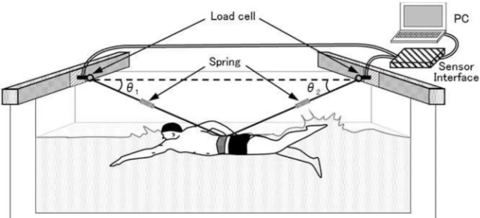
only the horizontal component forces, the angles of inclination of each wire, θ1 and θ2 (Fig. 1), were
considered. In all trials, swimmers used a snorkel to eliminate the influence of the breathing motion,
and all of them wore the same type of swimsuit to avoid a difference in the resistance because of
the swimsuit type.
Active drag was evaluated for the front-crawl swimming stroke using the new methodology
for estimating drag in swimming (MRT). Regarding the targeting swimming velocity for estimating
the active drag (VSi), we adopted five-staged velocity from i = 1.0 to 1.4 m s−1. All stages were measured on the same day and the participants were provided with enough rest to deal with the
influence of fatigue. Table 2 illustrates an example of a measurement procedure using the stage with
i = 1.00 m s−1 (V
S1.00). In deriving a regression equation from Eq. (7), we made the assumption that
the swimmer must be able to maintain the same technique, i.e., the same stroke rate, at VS1.00 within
the range of 0.80 U 1.20 m s−1. Thus, each swimmer was instructed to maintain the stroke motion and stroke rate SR1.00 at VS1.00 even when U was changed. The SR1.00 value was measured while each
swimmer swam at VS1.00. It was then calculated from the reciprocal of the 10-stroke time (defined
as the duration of 10 strokes, which was timed from the entry of the right hand on the first stroke to
the entry of the same hand after the 10th stroke). To make it easy for the swimmer to maintain the
Age Height Mass
(year) (cm) (kg) (s)
A 21 170 63 51.5
B 19 177 72 52.5
C 21 169 70 52.5
D 19 173 77 52.9
E 21 169 59 53.0
F 19 169 63 53.2
Mean 20.0 171.2 67.3 52.6
SD 1.0 3.0 6.2 0.6
6
motion and SR1.00 at different U values, the swimmer relied not on his own subjective senses but on
a sound that had the same interval as SR1.00, which was produced using a small waterproof
metronome (FINIS Inc., USA). As indicated in Fig. 2, using this procedure, swimmers were indeed
able to maintain a constant stroke rate equal to SR1.00 (at VS1.00) when U was changed; this was true
for all investigated speeds (VSi). To measure Tre at each value of U (0.80 U 1.20 m s−1), the
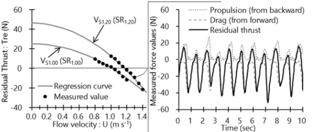
swimmer was towed in both directions (Fig. 3). The forward (D) and backward (P) forces were measured for 10 s after steady-state conditions were attained (measurements were started from the
entry phase of the right hand). Then, Tre was calculated from the difference between the forward
and backward towing forces (Fig. 4, right panel). The average values of Tre over 10 s were calculated
and used in the analysis. Best-fit regression curves were derived for the measured values of Tre by
adjusting the coefficient and constant terms in Eq. (7) (i.e., kD, kP, and VP) using the method of least
squares (MATLAB 2014a, Math Works Inc.). Finally, the active drag (Da) was derived by substituting kD and UTre0 (Tre intersecting the x-axis at zero in Eq. (7)) when the swimmer swam at
VS1.00. Furthermore, Da values at other VSi velocities were derived using the same procedure. As shown in the left panel of Fig. 3, kD, kP, and VP changed with VSi, and the swimming motion since Assumption 2 applied only when the swimmer maintained the same swimming motion. To
investigate the variability of MRT, Da at VS1.20 was estimated five times over three days for two
swimmers. The coefficients of variability for Da, UTre0, and SR1.20 were calculated from the ratio of
each standard deviation to each mean value for the five trials at VS1.20.
Passive drag (Dp) was measured by towing the swimmers, who maintained streamlined positions. The swimmers were towed forward and the forces were measured for 5 s at values of U
ranging from 0.9 to 1.5 m s−1 in 0.1 m s−1 intervals. To compare Dp and Da for the same swimmers,
7
Table 2. Measurement procedure using the stages of i = 1.00 m s−1 (V
S1.00). Initially, the stroke rate (SR1.00) and swimming motion at U = 1.00 m s−1 (V
S1.00) are examined. The swimmer is then instructed to maintain
the stroke motion and stroke rate SR1.00 at different flow velocities (0.80 U 1.20 m s−1).
Trial no. Flow velocity
: U (m s−1) Notes
1 1.00 Measured
stroke rate (= SR1.00)
↓ Maintain the specified stroke technique and SR1.00 ↓
2 0.80
3 0.85
4 0.90
5 0.95
6 1.00
7 1.05
8 1.10
9 1.15
10 1.20
Fig. 1. Bird’s eye view of the measurement process. A swimmer is towed in both directions and is
connected to each load cell through non-elastic wires. The forces measured in both directions are
processed through a sensor interface, which is linked to a load cell sampled at 50 Hz, and is inputted to
a personal computer. Furthermore, springs are used to prevent slack in the wire, caused by fluctuations
in the longitudinal direction, and the effects of tension caused when a swimmer alternates acceleration
8
Fig. 2. The results of the stroke rate at VS1.00 and VS1.20 (corresponding to Fig. 3) over several flow velocities (U) for swimmer A. The results of SR1.00 and SR1.20 evaluated from motion analysis were 0.45 0.01 Hz (coefficient of variation: CV = 0.6%) and 0.53 0.01 Hz (CV = 1.0%), respectively. Therefore, we
considered that Assumption 2 was valid from the standpoint of the near-constant SR.
Fig. 3. Relation between flow velocity U and residual thrust Tre at VS1.00 and VS1.20 (left panel) and measured force values at U = 1.30 m s−1 (right panel) for swimmer A. In the right panel, T
re (the solid
line) is calculated by subtracting the forward towing forces (defined as drag; dashed line) from the
backward towing forces (defined as propulsion; dotted line). Then, in the left panel, the regression curve
9
3.Results
The active drag (Da), velocity at Tre = 0 (UTre0), coefficient of drag (kD), and stroke rate (SR) for
each swimmer over five stages are shown in Table 3. In addition, Da and Dp for each swimmer is shown in Fig. 4. Moreover, the D vs. v relations in passive and active conditions were calculated for each subject and are also shown in Fig. 4. When pooling together data from all subjects, the relations
can be expressed as Da = 32.3 v3.3, N = 30, R2 = 0.90, and Dp = 23.5 v2.0, N = 42, R2 = 0.89. We
would report, in this Fig. 4, only the regression lines (both for Da and Dp) not the individual equations.
In the results on the variability in Da at VS1.20 for two swimmers, Swimmer A had a
variability of 6.5% (48.1 ± 3.1 N), whereas Swimmer B had a variability of 3.0% (48.7 ± 1.4 N).
Furthermore, the variability in UTre0 was 2.2% (1.15 ± 0.03 m s−1) and 2.3% (1.15 ± 0.03 m s−1),
and that of SR1.20 was 2.1% (0.52 ± 0.01 Hz) and 1.1% (0.48 ± 0.01 Hz) for Swimmers A and B,
respectively.
Table 3. Results of active drag (Da: N), calculated velocities from the regression curve (UTre0: m s−1), coefficient of drag (kD), and stroke rate (SR: Hz) for each swimmer at five-stage velocities ranging from 1.0 to 1.4 m s−1.
Da UTre0 kD SR Da UTre0 kD SR Da UTre0 kD SR
(N) (m s-1) (Hz) (N) (m s-1) (Hz) (N) (m s-1) (Hz)
1 25.1 1.02 24.3 0.45 28.6 0.95 31.5 0.41 28.4 0.98 29.4 0.40
2 42.9 1.09 36.4 0.46 40.8 1.13 32.2 0.44 50.3 1.11 40.8 0.41
3 46.4 1.17 33.7 0.53 48.6 1.19 34.6 0.49 62.7 1.16 46.4 0.45
4 54.3 1.21 37.2 0.57 55.0 1.23 36.2 0.56 73.9 1.22 49.6 0.50
5 84.2 1.34 47.0 0.70 73.2 1.37 39.0 0.69 95.3 1.37 51.0 0.59
Da UTre0 kD SR Da UTre0 kD SR Da UTre0 kD SR
(N) (m s-1) (Hz) (N) (m s-1) (Hz) (N) (m s-1) (Hz)
1 26.8 0.95 29.5 0.43 49.7 1.09 41.8 0.41 31.8 0.99 32.6 0.41
2 43.7 1.09 36.9 0.46 54.0 1.12 42.9 0.42 45.9 1.06 40.5 0.43
3 54.7 1.19 38.8 0.49 66.3 1.18 47.7 0.45 53.5 1.13 41.8 0.49
4 69.9 1.27 43.5 0.56 89.0 1.30 53.0 0.51 68.0 1.24 44.2 0.56
5 100.4 1.39 51.8 0.64 103.3 1.38 54.2 0.59 84.0 1.34 46.6 0.65
Stage
A B C
Stage
10
11
4.Discussion
The variability in Da evaluated using MRT indicated differences for both swimmers (Swimmer A: 6.5%, Swimmer B: 3.0%). As for the cause, we believe that in reality, the variability in SR
influenced the variability in Da. Thus, it can be considered that Da as estimated using MRT was also impacted by the difference in SR, which was influenced by various factors such as the swimmers’ conditions and fatigue level. From a previous study on undulatory underwater swimming
which reported on the variability in human movement (Connaboy, Coleman, Moir, & Sanders, 2010),
we know that differences in motion are a common occurrence when the same swimmers repeatedly
perform the same trial. Thus, since Assumption 2 is technically valid only when a swimmer
maintains the same exact swimming motion and stroke rate, in reality, the change in the kinematics
influenced the variability in Da estimated using the MRT. For this reason, we consider the variability in this study to be caused by the influence of human error rather than any systematic error. Hence,
this new methodology can be considered to be capable of evaluating a correct Da value that reflects a swimmer’s condition during a given day.
Additionally, concerning the prerequisite for the MRT (Assumption 2: a swimmer maintains
a certain stroke while Tre is measured at different values of U), the maintenance of a certain stroke
by the swimmers was also confirmed by measuring the SR for each trial using a stopwatch and using visual confirmation, not just by setting the required frequency on the waterproof metronome. As
indicated in Fig. 2, using this procedure, swimmers were indeed able to maintain a fairly constant
stroke rate when U was changed. As an example, the coefficients of variation for data reported in this figure (SR1.00 and SR1.20 at VS1.00 and VS1.20, respectively, for one swimmer) were of 0.6% and
1.0%, respectively. Therefore, it can be assumed that Assumption 2 was valid experimentally
because the swimmers maintained a near-constant stroke in different flow velocities, with the small
variations in SR resulting in small variations in Da because of human error. Furthermore, in a preliminary experiment, we confirmed that the times of each stroke phase and movement pattern
were not altered for different values of U.
For Dp, our values are similar to those reported by others (e.g., Zamparo, Gatta, Pendergast and Capelli (2009); Chatard, Lavoie, Bourgoin and Lacour (1990)); indeed, as reported by Havriluk
(2007), the Dp data were very similar across different experimental procedures. Therefore, the validity of the apparatus and conditions in this study was confirmed. For Da, previous studies reported quite different results because of the differences in the anthropometric and technical
characteristics of the swimmers observed as well as because of the differences in the adopted
methodologies. All these adopted methodologies have their pros and cons (for a discussion on this
point, the reader is referred to papers by Sacilotto, Ball, and Mason (2014), Toussaint et al. (2004),
and Zamparo et al. (2009)). For these same reasons, despite the difficulty in directly comparing our
12
larger than Dp; this agrees with the findings of some previous studies (e.g., Di Prampero et al., 1974; Formosa et al., 2012; Gatta, Cortesi, Fantozzi, & Zamparo, 2015; Zamparo et al., 2009) but not with
others in which Da was reported to be equal (or even lower) than Dp (e.g., Hollander et al., 1986; Toussaint et al., 1988; Toussaint et al., 2004; Van der Vaart et al., 1987). As recently pointed out by
Gatta et al. (2015), Da should be expected to be larger than Dp. This is because the frontal projected area of Da when the swimmers perform a swimming motion to propel themselves forward is larger than the area of Dp in the streamlined position (the smallest frontal projected area against the traveling direction). The lack of a common finding in the determination of Da in swimming studies was indeed the reason why we wanted to establish a new methodology for evaluating drag in
swimming (MRT) by gathering findings about drag in swimming, i.e., active drag in various
situations (swimming styles and velocities). Furthermore, the results in this study indicate that the
values of Da obtained using the MRT were approximately proportional to the cube of the velocity and not the square. This is thought to be the cause of the changes in the swimming motion and
stroke rate when increasing VSi, contrary to Dp. Therefore, it is necessary to gain a further understanding of factors that influence Da by analyzing the relation between the kinematics and Da.
5.Future prospects
In this study, we evaluated active drag at various velocities for front-crawl swimming with lower
limb motion. However, the new methodology (measured values of residual thrust; MRT) is special
in that it is applicable to various swimming styles. Therefore, the evaluation of the active drag (Da) using MRT would allow us to compare Da for different swimming styles and motions (techniques) as well as to evaluate swimming efficiency by estimating physiological indices, e.g., oxygen uptake.
Hence, in the future, the evaluation of drag in swimming using MRT is expected to play a role in
establishing fundamental swimming data. It has the potential to provide swimmers and coaches with
beneficial information for improving swimming performance.
Conflicts of interest None.
Acknowledgments
This study was supported by a Grant-in-Aid for Scientific Research [15K12641] from the Japan
Society for the Promotion of Science.
References
Chatard, J., Lavoie, J., Bourgoin, B., & Lacour, J. (1990). The contribution of passive drag as a determinant of swimming performance. International journal of sports medicine, 11(5), 367-372.
13
in the kinematics of maximal undulatory underwater swimming. Medicine and science in sports and exercise, 42(4), 762-770.
Di Prampero, P., Pendergast, D., Wilson, D., & Rennie, D. (1974). Energetics of swimming in man. Journal of applied Physiology, 37(1), 1-5.
Formosa, D. P., Toussaint, H., Mason, B. R., & Burkett, B. (2012). Comparative analysis of active drag using the MAD system and an assisted towing method in front crawl swimming. Journal of Applied Biomechanics, 28, 746-750.
Gatta, G., Cortesi, M., Fantozzi, S., & Zamparo, P. (2015). Planimetric frontal area in the four swimming strokes: Implications for drag, energetics and speed. Human movement science, 39, 41-54.
Havriluk, R. (2007). Variability in measurement of swimming forces: a meta-analysis of passive and active drag. Research quarterly for exercise and sport, 78(2), 32-39.
Hollander, A., De Groot, G., van Ingen Schenau, G., Toussaint, H., De Best, H., Peeters, W., Meulemans, A., & Schreurs, A. (1986). Measurement of active drag during crawl arm stroke swimming. Journal of Sports Sciences, 4(1), 21-30.
Kolmogorov, S., & Duplishcheva, O. (1992). Active drag, useful mechanical power output and hydrodynamic force coefficient in different swimming strokes at maximal velocity. Journal of Biomechanics, 25(3), 311-318.
Sacilotto, G., Ball, N., & Mason, B. R. (2014). A biomechanical review of the techniques used to estimate or measure resistive forces in swimming. Journal of Applied Biomechanics, 30, 119-127.
Toussaint, H., De Groot, G., Savelberg, H., Vervoorn, K., Hollander, A., & van Ingen Schenau, G. (1988). Active drag related to velocity in male and female swimmers. Journal of Biomechanics, 21(5), 435-438.
Toussaint, H., Roos, P. E., & Kolmogorov, S. (2004). The determination of drag in front crawl swimming. Journal of Biomechanics, 37(11), 1655-1663.
Van der Vaart, A., Savelberg, H., De Groot, G., Hollander, A., Toussaint, H., & van Ingen Schenau, G. (1987). An estimation of drag in front crawl swimming. Journal of Biomechanics, 20(5), 543-546.
14
Appendix
The coefficient and constant terms in Eq. (7) are replaced with , , and :
U U
Tre 2 (8)
That is, D P k k (9) P P 2k V
(10)
2 P P V k
(11)From Eq. (9), P D k
k (12)
where kP is derived from Eqs. (10) and (11);
4 2 P k (13)When Eq. (13) is substituted into Eq. (12), kD can be expressed in terms of α, , and .
4 2 Dk (14)
We derived the coefficient and constant terms in Eq. (8) (i.e., α, , and ) by best-fitting the measured values of Tre using the method of least squares (Fig. 3, left panel). Accordingly, the active drag (Da)
was derived by substituting kD and UTre0 (Tre intersecting the x-axis at zero in Eq. (8)) into Eq. (1)