VR Earthquake Experience System with Automatic Reconstruction of Indoor Environment

(1)

Graduate School of Energy Science, Kyoto University

Master Thesis in Socio-Environmental Energy Science

VR Earthquake Experience System

with Automatic Reconstruction

of Indoor Environment

Supervisor: Prof. Hiroshi Shimoda

Author: Daiki Handa

(2)

Abstract

Title:

VR Earthquake Experience System with Automatic Reconstruction of Indoor Environment

(室内環境の自動再構築手法を用いた VR 地震体験システム)

Shimoda Laboratory, Daiki Handa

Abstract:

As 2011 Tohoku Earthquake represents, earthquakes could cause enormous human casualties, and it is crucial to reduce their risks through disaster education. One important approach is to increase preparedness towards earthquake by causing fear toward it, under the principle of fear-arousing communications. Various immersive earthquake simulation methods has been developed to serve this purpose. Of these methods, a method based on virtual reality (VR) is attractive, because it only requires a compact hardware unlike simulation vehicles, and it has a potential to be widely adopted. But the contents need to be created manually by artists, and that limits its practicability.

In this research, a new earthquake experience system is proposed in which indoor environments are 3D-scanned, and a virtual environment is automatically created by a novel reconstruction method. Simulation of earthquakes is presented via VR. It can be expected the proposed system removes the cost problem of the previous VR method, while still retaining eﬀectiveness in fear-causing.

To examine whether the system is actually capable of causing fear toward earthquake, an experimental evaluation was conducted. In the experiment, participants experienced earthquakes simulated by the system, and perceived fear, realness, and seismic intensity scales were measured by questionnaires, among other properties. Interviews were also conducted to investigate factors aﬀecting these perceptual properties. The evaluation ex-periment showed that an earthquake simulation of seismic intensity scale 6.6 could actually cause fear in more than half participants. However, perceived seismic intensity scales were consistently lower than simulated intensity scales. The interview results revealed that the discrepancy could be attributed to omission of vestibular stimulus and lack of details in reconstructed scenes. Of several elements contributing to realness, ground-shaking sounds and overall scene photorealism were scored moderately high. However, collision sounds of objects were felt as unrealistic, because of lacking detail in object recognition.

Although the automatic approach of the proposed system was shown to be viable, increasing reliability and granularity of object recognition would be a hard problem, and would need signiﬁcant progress in the ﬁeld of computer vision.

(3)

List of Figures

2.1 Two factors in fear-arousing communications. . . 4

2.2 Workﬂows to generate VR contents in a conventional (left) and the pro-posed (right) method. . . 7

2.3 Conceptual dataﬂow in reconstruction. . . 8

2.4 Four types of image understanding. . . 8

2.5 An example of distance image of a room. Brightness of each pixel is pro-portional to the distance between the camera and a point on a 3D surface pointed by the pixel. . . 9

3.1 System requirements and functions of three subsystems. Arrows depict depends-on relations. . . 11

3.2 Dataﬂow between subsystems. . . 12

3.3 A point cloud obtained by the scanning subsystem, at a single scan location. 12 3.4 Diﬀerence of nodes (shown as black dots) between a FEM simulation (left) and a rigid body simulation in a proposed system (right). . . 14

3.5 Phenomena in an earthquake and corresponding sensory modes. . . 16

3.6 Photo of the 3D scanner. . . 17

3.7 Operation principle of LRF. . . 17

3.8 Fields of view of the sensors when not rotated. . . 18

3.9 Operation of scanner (top view). . . 18

3.10 A solid angle covered by a single RGB image. . . 19

3.11 Equirectangular projection of spherical coordinates. . . 20

3.12 A single RGB image warped to equirectangular coordinates. . . 20

3.13 Stitched RGB image. . . 21

3.14 Stitched RGB image with color correction. . . 21

3.15 Resampling artifacts of distance images. . . 22

3.16 A view of a ﬂat region in a point cloud, showing errors of a few centimeters. The ﬂat region is highlighted in orange. . . 23

3.17 Distance image D. Pixel brightness is proportional to distance. . . 23

3.18 Normals calculated from raw distance image. (XYZ components are visu-alized as RGB color.) . . . 24

3.19 Intensity of reﬂected infrared light. . . 24

3.20 Normals calculated from ﬁltered raw distance image. . . 25

3.21 A point cloud generated from 3D scan data at a single location. . . 25

3.22 Dataﬂow of indoor reconstruction pipeline. . . 26

(6)

3.24 Multiple paths from a node to another in a graph (left). There is only

single path between nodes in a tree (right). . . 30

3.25 A minimum spanning tree of the point clouds. Each node is a point cloud, and each edge is dinv between two point clouds. . . 31

3.26 2D projection of a merged point cloud, consisting of 4,065,020 points. In this 7 m_{× 4 m oﬃce, 15 scan data were taken. . . 32}

3.27 2D Points after ﬁltering. . . 32

3.28 A concave hull extracted from a ﬁltered points. . . 33

3.29 Vertical bands on a ﬂat region, caused by noisy normals. . . 33

3.30 Samples (input values) and clusters, seen from the AIC perspective. . . 34

3.31 Detected Manhattan frame. . . 35

3.32 Quality of image at various points on the ceiling. . . 35

3.33 Images projected to the ceiling, containing 4 ﬂuorescent lights. Left: Color, Right: binary after threshold. . . 36

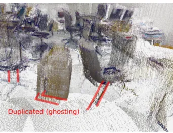
3.34 Ghosting errors in a point cloud. Legs of chairs, and surface of a box are duplicated. . . 36

3.35 Three steps in patch extraction. . . 37

3.36 Patches from a single scan location, colored by cluster. . . 38

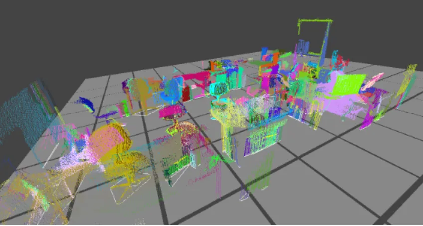
3.37 All patches from a single room. This particular example has 405 patches in total from 15 scan locations. . . 39

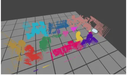
3.38 An object is stable when its center of gravity falls inside the support polygon. 39 3.39 Final stable patch clusters. . . 41

3.40 A 3d triangle mesh (left), and triangles unwrapped in UV coordinates (right). Orange lines denote UV mapping. . . 42

3.41 The texture of the interior boundary (left) and a zoom of the ﬂoor (right). Most of the ﬂoor is occupied by distorted objects. . . 43

3.42 Relationship between distance between the scanner and surfaces, and in-valid regions. . . 43

3.43 From left to right: a, b,∥a − b∥. X, Y, Z components of 3D position is represented by R,G,B colors, and distance is represented by brightness. . . 44

3.44 Masks used for invalid region identification (red: invalid floor, green: valid floor), before adjustment (left) and after adjustment (right). . . 44

3.45 Floor parts of textures before invalid region detection (left) and texture after inpainting (right). . . 44

3.46 Generated textured mesh and collision shape for an interior boundary. Collision OBBs are shown as purple boxes. . . 45

3.47 An example of generated textured object for an object. (left: before texture generation, right: after texture generation) . . . 46

3.48 An example of textured mesh and collision shape generated for an interior object. . . 47

3.49 Top row: photos of each scene. Bottom row: reconstruction, rendered by the runtime subsystem. From left to right: un1, re1, re2, and re3. . . 49

3.50 Ceiling images of re3 (left) and un1 (right). Red circles denote a bright region with no light ﬁxture. . . 49

3.51 20 objects manually counted in a part of an RGB image. . . 50

(7)

3.53 Example results of collision sound extraction. Green boxes denote

ex-tracted parts of the sounds. . . 52

3.54 A headphone, an HMD and a tracking camera. . . 54

3.55 An artist-created example of indoor scene running in a state-of-the-art game engine. . . 55

3.56 Loudness of collision sounds vs. relative velocity between the two colliding objects. . . 56

4.1 Requirements of the system. . . 58

4.2 Photo of the HMD. . . 59

4.3 Experimental protocol of a single group (1.5 hr). . . 61

4.4 Side-view of the participant and apparatus. . . 63

4.5 A photo of the experiment. The person in the middle is a participant, and the other person is an experimenter. . . 63

4.6 A virtual ﬂoating screen asking the level of fear. . . 64

4.7 Histogram of maximum earthquake seismic intensity scale experienced by participants in the past. 0 denotes no experience. . . 66

4.8 Perceived seismic intensity scale vs. simulated seismic intensity scale. . . . 67

4.9 Perceived fear for each simulated scale. . . 67

4.10 Means and standard deviations of scores for each element of the realness. Error bars denote standard deviations. . . 68

4.11 Histogram of sickness during the experience. . . 69

4.12 A part of wall (a ﬂat vertical plate on the right) mistakenly included in an interior object. . . 70

A.1 A triangle mesh (left) and the UV coordinates of the vertices (right). . . . 82

B.1 Seismic intensity scales and descriptions . . . 85

B.2 Pre-VR questionnaire page 1. . . 86

B.3 Post-VR questionnaire page 1. . . 87

B.4 Post-VR questionnaire page 2. . . 88

B.5 An illustrated table to help participants remember seismic intensity scales, rearranged to increase visiblity in VR. . . 89

(8)

List of Tables

2.1 Various methods of earthquake information presentation. . . 4

3.1 Speciﬁcation of the RGB camera in the scanner. . . 17

3.2 Speciﬁcation of the LRF in the scanner. . . 18

3.3 Speciﬁcation of the servo motor in the scanner. . . 18

3.4 Scanned indoor scenes and their descriptions. . . 47

3.5 Reconstruction results and time to process the scenes. . . 48

3.6 Processing time of reconstruction broken up in several parts. . . 48

4.1 Speciﬁcation of the HMD and the tracking system. . . 58

4.2 Speciﬁcation of the noise-canceling headphone. . . 59

4.3 Speciﬁcation of the controller PC. . . 59

4.4 Used seismographs and their maximum seismic intensity scales. . . 60

4.5 Description of seismic intensity scales used in the experiment. . . 62

4.6 Questions on elements of realness in questionnaire Q3. . . 65

4.7 Questions about perceived seismic intensity scale, fear, memorability, and VR sickness, in questionnaire Q2 and Q3. . . 66

4.8 7-Level Likert scale and corresponding numeric scores. . . 68

C.1 All interview answers. . . 90

C.2 Free comments. . . 95

C.3 Answers to Q1 and Q2. . . 96

(9)

Chapter 1 Introduction

The 2011 earthquake oﬀ the Paciﬁc coast of Tohoku had caused enourmous human casualties. Since earthquakes occur frequently, natural disaster education plays an im-portant role in reducing their risk.

A critical aspect of the disaster education is to persuade people to actually prepare for earthquakes through fear-arousing communication[1]. There are three methods to cause fear towards earthquakes: video footages of an earthquake, simulation vehicles, and virtual reality (VR) earthquake simulation[2].

Video footages are widely used since they can provide variety of both indoor and outdoor situations relatively easily. But they are arguably the least effective in causing fear, because watching a video on a screen is not immersive. Simulation vehicles are also commonly used, and they can simulate an earthquake in a small room. A simulation vehicle is a small truck containing a shake table and a small room attached to it. People can experience earthquakes by getting inside it, surrounded by the room and furnitures. Although the experience is very immersive, its realness and flexibility are limited. First, the furnitures must be secured in place to prevent injuries by toppling over people, and simulation of a large room is difficult because of vehicle size. Second, changing the room to different situations is also hard, because physical installation must be changed when-ever situation is modified. The VR earthquake simulation[2] is a proposal to display an earthquake in a virtual indoor scene, simulated by computers. In theory, it can simulate any kind of scene and present it immersively by using VR hardware that occupies users’ field of view entirely. However, it is hard to simulate many kinds of scenes because of the cost and time required to model furnitures and buildings professionally.

Thus, there are no existing method that can simulate earthquakes in a variety of indoor scenes with high immersiveness, and at lower cost. Of these three methods, the VR earthquake simulation method has arguably the largest potential, because its limiting factor is cost of content generation, unlike other methods which are limited physically.

(10)

Meanwhile, ﬁelds of computer graphics, computer vision, and virtual reality are rapidly progressing, backed by constantly rising computational power, represented by the Moore’s law. Two interesting developments are, gradual availability of high quality VR hardware at consumer prices, and progress of 3D reconstruction techniques in general.

In this research, a new VR earthquake experience system is proposed, which is based on automatic generation of 3D contents from 3D scan data. In the previous method, individual objects in an indoor scene are manually modeled by professional artists, and then motion of the objects are calculated via physics simulation by computers. In the proposed system, such a manual modeling process is replaced by a novel automatic re-construction method, eliminating the cost problem. The rere-construction method takes 3D scan data of target indoor scene as an input, recognizes objects contained in the data, and then reconstruct appearance and physical models of the objects. Existing methods[3][4] are typically capable of only one of recognition and reconstruction, and are incapable of generating 3D contents for physics simulation. Due to the low cost and automatic nature of the proposed system, it would be able to scan and generate the contents where earth-quake education is being conducted, such as schools or public meetings. This is a unique property of the system unlike previous methods, where target scene must be prepared beforehand.

The proposed system was evaluated by an experiment, in which participants experi-enced the earthquake contents generated by the system, and feedbacks were collected via questionnaires and interviews.

The thesis consists of 5 chapters including Introduction. In chapter 2, the background of research is discussed and existing 3D reconstruction techniques are reviewed. In chap-ter 3, the proposed system is described as a composition of three subsystems and various methods that consist them, including the new indoor reconstruction method. In chapter 4, an experiment is devised from the fear-arousing communication principle and the system requirements, and the experiment results are analyzed. Finally, chapter 5 summarizes the research and discusses future works to further enhance eﬀectiveness of the system.

(11)

Chapter 2 Background and Objective of This

Research

In this chapter, we review existing methods of information presentation used in earth-quake education, from Disaster Risk Reduction (DRR) and fear-arousing communication perspectives. Then we propose a new VR earthquake experience system based on auto-matic content generation and realtime computer simulation, while mentioning existing literature on 3D scene understanding.

2.1 Existing Earthquake Education Methods

In literature of DRR, Wisner et al. proposed CARDIAC, which is a set of seven con-crete objectives for risk reduction[5]. One of CARDIAC objectives is Communication, which is described as to “Understand and communicate the nature of hazards, vulnera-bilities and capacities.”[5]. Education of disaster can be considered to be one approach to the communication objective. But the literature also states that eﬀective DRR requires not only informing people about disaster, but also changing actual behavior of people.

One such method of changing behavior is fear-arousing communication[1]. Fear-arousing communication is comprised of 1. fear toward the risk, and 2. knowledge of actions to reduce the risk, and it is known that such a combination increases attitude and action toward the risk. Fig. 2.1 shows this relationship. In case of earthquake, there are several methods of information presentation, which are summarized in Table 2.1 with qualitative evaluation of amounts of informational content and fear caused by the meth-ods.

Text-based method presents information via text and images usually on printed paper, and can convey large amounts of complex information such as mechanism and history of earthquakes. However, it is diﬃcult to arouse fear via use of text-based methods.

(12)

Video-Figure 2.1: Two factors in fear-arousing communications. Table 2.1: Various methods of earthquake information presentation.

Type of presentation Information Fear

Text-based[6] high low

Video-based[7] mid-high low-mid Simulation vehicle[8] low high

VR[2] low high

based method is typically a mixture of recorded disaster footage and descriptive part much like text-based presentation. Thus, video-based method can arouse medium amount of fear with low information content, or low fear with high information content.

On the other hand, simulation vehicles or VR earthquake simulation are mainly de-signed to cause fear by their immersiveness, rather than to present information. Also, simulation vehicles are limited to indoor scene. Arguably, it is harder to deploy these methods compared to text-based or video-based methods, because of higher cost required to prepare simulation vehicles or professionally created 3D contents for VR.

These two groups of methods correspond to the two complementary factors in fear-arousing communication (Fig. 2.1), and they are also used in a mixed way in practical earthquake education settings. However, the immersive methods are limited in variation of indoor scenes they can present, primarily because of their high cost. Section 2.2 discusses these methods more closely.

2.2 Immersive Earthquake Experiences

A typical earthquake simulation vehicle is equipped with a single small room on a shake table, in which several people can experience earthquake simulataneously[8]. It is common for such a vehicle to be able to simulate earthquakes up to scale 7 (using Japan Meteorological Agency seismic intensity scale[9]). Seismic intensity scale 7 can be thought of as the maximum seismic intensity scale practically required for an indoor earthquake experience system, since it is estimated that most buildings will collapse in an earthquake

(13)

stronger than scale 7. It is also technically possible to increase the size of simulation up to a whole building, using a huge shake table such as E-Defense[10].

Although simulation using mechanical shake tables can generate completely accurate experience in theory, they are practically limited by safety and cost constraints. For example, furnitures need to be secured in place to avoid physical harms to the subjects, and simulation of multiple or larger environments is hard due to the cost associated with the physical setup. These constraints hinder realness, because objects such as furnitures can move above seismic intensity scale 4, and this method cannot simulate them. Below scale 4, the value of earthquake simulation is low, because weak earthquakes are pretty harmless to human and also occur relatively frequently.

Another type of immersive earthquake simulation[2] can be created with VR which relies on electronic hardware such as head mounted display (HMD) and headphones to stimulate human senses, and computer to simulate physical process. In this case, environ-ment can be anything within the limit of computation, so the problems of environenviron-ment size and non-moving furnitures can be resolved.

However, there are two technical problems with the existing VR method. First, sensory modes of stimulus are typically limited to visual and auditory because other modes such as touch and olfaction, are much less understood and hard to synthesize. An excluded sensory mode of particular importance is vestibular sense, which is used to sense acceleration and rotation of head. Vestibular system can be stimulated by using motion platforms, which are essentially same as shake tables. Mixed setup of motion platforms and audio-visual VR hardware is commonly found in aircraft pilot training[11], but there is no known work for earthquake experience utilizing such a setup. Second, 3D content creation by artists can be costly, possibly more than purchasing real furnitures. In a tutorial website for 3D artists[12], it is stated that an artist should charge 500 USD for an empty room, and 50 USD for a single simple object such as a wooden box. Considering a typical room contains hundreds of unique objects (e.g. furnitures, tools, books, clothes) with shapes more complex than a box, it can be argued that modeling a room costs more than 5500 USD.

Both the limitations of simulation vehicles and the lack of vestibular or tactile senses in VR stem from physical constraints, and arguably these disadvantages are hard to overcome. However, cost of 3D content creation in the VR method could be lowered drastically by automatic content generation.

(14)

2.3 Objective of This Research

In this research, we propose a system that can generate content automatically and can simulate earthquake in VR using the generated content. Since the system is automatic, it can eliminate the cost problem in existing VR earthquake simulation methods, and also enables modeling of various locations, including a site where earthquake education is con-ducted. These properties of the system would help spreading VR earthquake simulations, which are conceivably eﬀective in causing fear because of its high immersiveness.

Ability of the system to cause fear and practicability of the system are also evaluated experimentally in this research.

2.3.1 Proposed Earthquake Experience System

The proposed system can generate content automatically and use the content for VR earthquake experience. The automatic generation is enabled by a novel indoor 3D reconstruction method which can generate separated objects with both appearance model and collision model for rigid-body physics simulation, unlike existing 3D reconstruction methods reviewed in section 2.4.

The proposed system is expected to be usable by a non-professional person to scan a real indoor scene, and generate content for earthquake experience of the scene auto-matically, given measured earthquake data to simulate. Combined with availability of high-quality HMD at consumer prices such as Oculus Rift DK2[13], the system can be expected to be used to scan a real world location, and to present the experiences of the location. The location could be where earthquake education is conducted, or residence of the educatee to enhance the fear.

Fig. 2.2 shows the difference in content creation workflows between the conventional method and the proposed system. Vast reduction of time consuming and costly pro-fessional labor is apparent in the proposed system. Due to the difficulty of perfectly recognizing objects and phenomena in the scene, the proposed method will not be able to generate complex phenomena such as building deformation, wall cracking, or object shat-tering. However, the potential of the proposed method to present on-the-spot experience can be considered to overweigh these disadvantages in realness.

2.4 Existing Literatures on 3D Scene Reconstruction

To reconstruct a real world scene, the scene must be captured by cameras or 3D scan-ners, and then various properties of things in the scene must be estimated by computers. These properties include 3D object locations, materials, and light locations. Extraction

(15)

Figure 2.2: Workﬂows to generate VR contents in a conventional (left) and the proposed (right) method.

of information like this is called scene understanding. Then, these properties must be converted to forms suitable for realtime rendering and simulation. Typically, objects are represented by triangle meshes and textures. Finally, the objects and the lights are placed in a virtual scene, and the physical phenomena such as earthquakes become simulatable. Fig. 2.3 shows this conceptual dataﬂow of scene reconstruction.

An ideal computer vision program would be able to very deeply recognize all objects in an arbitrary image, which means it could estimate all of the following:

• which object a given pixel corresponds to (segmentation) • linguistic properties (e.g. name) of the objects

• kinetic properties (e.g. mass, rigidity, articulation) of the objects • visual properties (e.g. color, 3D shape, surface material) of the objects

Fig. 2.4 shows these four concepts visually. However, complete recognition of objects in an arbitrary scene is believed to be the hardest problem in computer vision[14], and existing state-of-the-art methods typically focus on only one or two of these aspects and still yield incomplete results. Existing methods are grouped by their primary aspects, and are reviewed brieﬂy in the following.

(16)

Figure 2.3: Conceptual dataﬂow in reconstruction.

Figure 2.4: Four types of image understanding.

Existing methods[15][16] that can do segmentation require distance information from a depth camera like kinect, or a laser range finder (LRF). These special cameras can obtain distances between the camera and surfaces in each direction. Fig. 2.5 shows one of such result. It is easier to estimate or fit 3D shapes using such distance information compared to RGB images, because RGB images are heavily influenced by lighting conditions and surface materials while distance is not affected by lighting. In these methods, objects are segmented by fitting simple geometric shapes or finding repetitive shapes. However, these methods do not produce appearance models usable for synthesizing images, nor guarantee any physical correctness of the segmentation.

There are other methods that can output names of objects in an RGB image. Some can only recognize a single object occupying a whole image[17], and another can recognize

(17)

Figure 2.5: An example of distance image of a room. Brightness of each pixel is propor-tional to the distance between the camera and a point on a 3D surface pointed by the pixel.

approximate 2D locations of multiple objects as bounding rectangles[18]. However, they cannot output any models for rendering or physical simulation, and the detection is far less reliable than the previous group of segmentation methods based on 3D input data.

Another set of methods apply physical reasoning to 3D input data such as distance images, and try to extract physically plausible configuration of objects along with shape of each object[3][19][20]. Physical plausibility of object configuration is twofold. First, no objects should be intersecting with each other. Second, all objects should be stable at the initial state, which means all objects should be at local minima of potential energy. The latter condition is typically satisfied by all objects being supported by the floor either directly or indirectly. In one of the advanced methods[19], potential energy is explicitly minimized when estimating object boundary, and the method even outputs approximate shape of each object as voxels. However, the output shape is rough compared to dedicated segmentation method, and constructing a visual appearance model from such a rough model is relatively hard.

The last kind of methods[21][4] focuses on generating good-looking visual appearance model with little or no segmentation. Which means all objects in the scene are glued to-gether, making it impossible to physically simulate behavior of individual objects. There is a method that can generate relatively clean geometric shape models of multiple ob-jects[22], but the method requires manual interaction to specify approximate boundary of objects in images.

In the proposed system, a new reconstruction method to extract roughly segmented objects with visual appearance models, which also satisﬁes physical plausibility condition, is required. The reconstruction method approaches this hard problem by limiting the type of scene to a single room and using prior knowledge about such environment, rather than formulating it as a general problem.

(18)

Chapter 3 VR Earthquake Experience System

In this chapter, we closely look into the requirements and functions of the system, while considering various trade-oﬀs between cost and realness. And then we propose a novel indoor reconstruction method, and a way to integrate a generated scene model and earthquake data into a virtual earthquake in VR.

3.1 Requirements and Functions of the VR

Earth-quake Experience System

As described in subsection 2.3.1, the ultimate goal of the proposed system is to cause fear toward earthquake, as part of fear-arousing communication, by providing an immer-sive earthquake experience via automatic scene reconstruction. The system only considers visual and auditory senses, because most other senses such as touch and olfaction are not strongly affected by a typical earthquake. Although the vestibular sense (i.e. feel of ac-celeration) is heavily affected by an earthquake, it is omitted because reliably stimulating it requires a large and expensive motion platform. Subsection 3.1.1 and subsection 3.1.2 discuss such trade-offs between realness and cost, from aspects of content generation and sensory stimulation, respectively.

The system goal is represented as two core requirements: automatic earthquake con-tent generation and ability to cause fear. Automatic earthquake concon-tent generation can be divided into two sub-requirements, ability to output diﬀerent scenes, and ability to vary seismic intensity scale. These sub-requirements are realized by data-driven approach. The system takes 3D scan data and earthquake data as inputs, and generates content based on the input. The other core requirement, ability to cause fear toward earthquake, consists of two sub-requirements, high realness of generated virtual scene and high memorability of the experience. The generated scene must represent earthquakes as relistic as possible,

(19)

because the system should cause fear toward earthquake, and not toward an arbitrary phenomena. Also, it is desirable the experience has high memorability, otherwise the system would be less eﬀective in fear-arousing communication.

There is one additional requirement, that the system should not cause VR sickness[23]. This is because severe VR sickness would prevent users from using the system and would nullify other capabilities of the system.

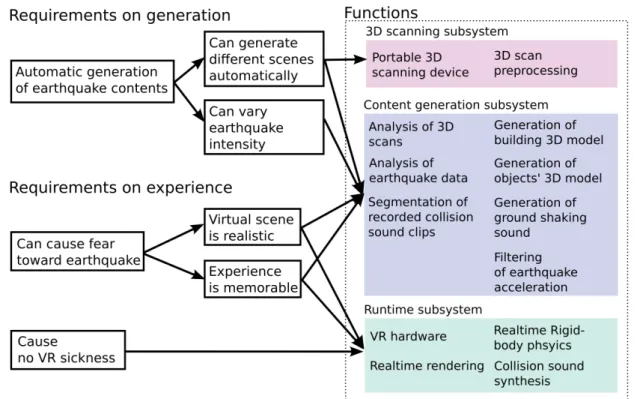
Fig. 3.1 shows the three requirements and four sub-requirements and their dependency. These requirements are implemented as three subsystems, because the system needs to 1. capture a real scene, 2. analyze (reconstruct) it, and 3. present it using VR, as shown in Fig. 3.2. The functions of three subsystems are described in the following.

Figure 3.1: System requirements and functions of three subsystems. Arrows depict depends-on relations.

The 3D scanning subsystem is a portable 3D scanning device with software to pre-process the scanned data to make it easier for the content generation subsystem to analyze the 3D indoor environment. The scanner can collect multiple RGB and distance images by rotating a camera and an LRF, resulting in nearly omnidirectional coverage. Prepro-cessing includes color and exposure correction, and noise removal, which is essential to reduce spurious object detection and increasing ﬁnal visual quality. The output of the subsystem is a collection of RGB and distance images in equirectangular coordinates, and 3D point clouds corresponding to diﬀerent vantage points in a target indoor environment. A point cloud is a collection of 3D points, with optional attributes like colors and normals.

(20)

Figure 3.2: Dataﬂow between subsystems.

Fig. 3.3 shows a point cloud obtained by the subsystem, and the point cloud contains col-ors and normals, but normals are not shown in the ﬁgure. The detail of the subsystem is described in section 3.2.

Figure 3.3: A point cloud obtained by the scanning subsystem, at a single scan location. The content generation subsystem is a software that combines 3D scan data obtained by the scanner and user-specified earthquake data, and generates 3D content for VR by applying various analysis methods. More specifically, the inputs of the subsystem are 3D scan data taken at multiple locations, measured earthquake acceleration sequence, and recorded collision sound clips. The outputs of the subsystem are 3D content, earthquake sound (i.e. ground shaking sound), pre-processed collision sounds, and filtered earthquake acceleration.

The 3D contents are multiple 3D objects roughly corresponding to furnitures (will be called interior objects) and a single 3D object to represent ceiling, ﬂoor and walls combined (will be called interior boundary). These 3D objects not only have appearance model to render them, but also collision models for realtime rigid-body simulation. Since the content generation subsystem is the largest part, its details are described in several sections as follows.

• 3D content generation from 3D scan data: section 3.3 • Collision sound preprocessing: section 3.4

(21)

• Earthquake acceleration filtering and ground shaking sound generation: section 3.5 The runtime subsystem consists of VR hardware such as a head mounted display (HMD) and a headphone, and software to feed data into the hardware. The software takes the data generated by the content generation subsystem, and simulates objects’ movement using filtered earthquake acceleration, and renders final visual and auditory stimuli to be fed into the hardware. These functions are enabled with a combination of a game engine and custom code. A game engine is a set of programs that provides a variety of functions in computer graphics, physics simulation, and VR hardware control. Since VR requires high framerate and stability to prevent VR sickness, earthquake-specific custom code is implemented on top of an existing game engine, which provides high quality implementation of the basic functions. Section 3.6 describes the details of the subsystem.

Design limitations of the system are discussed in the following subsections.

3.1.1 Aspects of Indoor Earthquake Modeled in the System

Quality and cost of graphics and sound contents would vary depending on whether they are created manually by artists, or automatically by a program. The diﬀerences forms a trade-oﬀ between high realness and low cost. The proposed system prefers the latter, because its goal is to cause fear toward earthquake in a inexpensive, thus easily adoptable way. However, there is a middle ground between fully manual and fully au-tomatic contents creation, such as placing manually created furnitures auau-tomatically by recognizing the objects in the scene. In this subsection, 3D and sound contents related to indoor earthquake situations are discussed, and the design choices of the proposed system are explained.

Before simulating an earthquake, an indoor environment without earthquakes need be simulated. In a typical room without an earthquake, almost all objects are stationary, and there are only quiet ambient sounds caused by things such as fans of electronic devices. A significant exception is people and objects around them. Although behavior of other people under earthquake might have significant effect on the users’ emotion including fear, they are omitted because simulation of people would add an insurmountable complexity to the system. Consequently, a real indoor scene is also assumed to be completely static and devoid of people while being scanned. Ambient sounds are also excluded from the simulation, because they would be inaudible because of auditory masking caused by much louder earthquake sounds.

When an earthquake occurs, the wave propagates through the ground and the build-ing, and to the objects inside the room. Acceleration measurements at the ground level are widely available via monitoring networks such as K-NET[24], but the transfer func-tion between the ground and the room is dependent on the building structure and other

(22)

factors. For example, it is known that resonance of a building to an earthquake could have significant impact on final motion[25]. In the previous earthquake simulation method[2], the final motions of the room and objects attached to it are calculated by finite element methods (FEM). The calculation is possible because structural model of the building is modeled manually in the previous method, allowing incorporation of material properties which are directly unobservable. In the proposed method, such reliance on external in-formation that cannot be recognized automatically is avoided. Thus, all buildings and objects as treated as rigid bodies, as shown in the right of Fig. 3.4. Under this approxima-tion, physics simulation can be further simplified by considering the room as an inertial frame with the acceleration equal to the acceleration measured on the ground, instead of objects shaken indirectly via moving floor. This simplification would increase stability and efficiency of rigid body simulation.

Figure 3.4: Diﬀerence of nodes (shown as black dots) between a FEM simulation (left) and a rigid body simulation in a proposed system (right).

When the earthquake waves reach the objects inside the room, several phenomena can occur. First, there would be a low frequency rumbling sound which is supposedly caused by ground shaking. Since there is an existing method[26] to synthesize this sound from accelerations, similar approach is taken in the proposed system. Second, small objects can tremble and make sounds, and furnitures can topple over and make large sounds when they hit the ﬂoor. These types of sounds can be generalized as collision sounds, and the motion can be simulated by rigid body simulation. Intuitively, the sounds are sum of short collision sounds caused by individual collisions. There is an existing method[27] that can create variations of recorded collision sounds for games. In the method, types of sounds are associated to types of objects manually, and the associated sound is played with slight random variation when an object collides. We take a similar approach, but since reliable recognition of types of objects is infeasible, a slightly diﬀerent method that can accommodate the uncertainty of types is proposed.

(23)

solely by rigid body physics. For instance, a cabinet door can spontaneously open and release its contents, a dish can shatter and produce numerous shards, or papers can fall from a desk and ﬂap in midair. As discussed in section 2.4, recognition of objects with this level of detail is completely beyond the current state of the art, thus ignored in the proposed system.

In summary, the proposed system recognizes objects in an indoor scene at a scale of furnitures (e.g. cannot separate individual book in a bookshelf), and apply rigid body simulation and a generic collision sound synthesis method without information of detailed physical properties of each type of objects. This would enable the following aspects to be simulated.

• Rough appearance of objects • Motion of objects (as rigid bodies) • Collision sounds

• Ground shaking sound

3.1.2 Sensory Modes Stimulated by the System

There is a similar trade-off between realness and low-cost, when selecting the sensory modes to be simulated by the system. Obviously, stimulating as many senses as possible would maximize realness. However, there is a difference in difficulty of stimulating various senses. For instance, stimulation of vestibular and proprioceptive senses would require large and expensive apparatus such as a motion platform and an exoskeleton, but it is much easier to stimulate visual and auditory senses by using HMD and headphone. In the proposed system, only visual and auditory senses are targeted to lower the cost of the system adoption.

Assuming the user would not interact with objects, tactile sense can be ignored. Fig. 3.5 summarizes the relationships between the other senses and various elements in static (i.e. not shaking) and dynamic (i.e. shaking) scene. Non-simulated elements and modes are shown in gray.

Among the discarded senses, vestibular and proprioceptive senses are relatively im-portant, because human can feel head acceleration and body posture by these senses. In a real earthquake, the whole body will be perceivably accelerated even in weak earthquakes, and the body posture would change in stronger ones. When simulating earthquake using VR, the acceleration and movement of the avatar, a virtual body of the user, should be reﬂected back to the real body so that the user can perceive a stimulus similar to that of real earthquake. However, known reliable methods to stimulate these senses are limited

(24)

Figure 3.5: Phenomena in an earthquake and corresponding sensory modes. to motion platforms and force-feedback exoskeleton, and there is a trade-oﬀ between real-ness and portability (or cost). In favor of the latter, we discarded these senses. Olfactory sense is omitted because it is rarely aﬀected by an earthquake.

3.2 3D Scanning of Indoor Environment

The 3D scanner hardware used in the proposed system was developed in our lab as part of an augmented reality research[28]. However, this research requires higher quality data, so additional preprocessing is introduced, which is described in subsection 3.2.2.

3.2.1 3D Scanning Device

The hardware of the 3D scanning subsystem is identical to the previously developed scanner hardware, used for simulation of indoor lighting change using augmented reality [28]. Fig. 3.6 shows the scanner and its main components. The scanner is approximately 30 cm tall.

The scanner contains two sensors, a wide-angle RGB camera, and a laser range finder (LRF). These two sensors are attached on top of a rotating platform. An LRF can be though of as a one-dimensional distance camera, which emits infrared laser to various directions and records intensity of the reflected light and time of flight. From the time of flight, distance between the LRF and a point on a surface can be calculated. The points swept by the LRF forms a curve, called a scanline. Fig. 3.7 shows this operation of an LRF.

(25)

Figure 3.6: Photo of the 3D scanner[28].

Figure 3.7: Operation principle of LRF.

Since neither the RGB camera nor the LRF covers the whole solid angle, the upper part of the scanner that contains two sensors is rotated by a servo motor to collect multiple images and scanlines at diﬀerent angles. Fig. 3.8 shows ﬁelds of view of both sensors when they are not rotating, and Fig. 3.9 shows rotation of the sensors in top view.

RGB images are collected at interval of 5◦, and LRF scanlines are collected at interval of 0.5◦. The scanner can cover most of the solid angle, except polar regions. Speciﬁcations of the RGB camera and the LRF are shown in Table 3.1 and Table 3.2. The speciﬁcation of the servo motor used to rotate them is also shown in Table 3.3.

Table 3.1: Speciﬁcation of the RGB camera in the scanner. Product name Asahi Electronics NCM13-K

Imaging device 1/4 inch CMOS Resolution 1280× 1024

Output format YUV422 / RGB565

(26)

Figure 3.8: Fields of view of the sensors when not rotated.

Figure 3.9: Operation of scanner (top view).

Table 3.2: Speciﬁcation of the LRF in the scanner. Product name Hokuyo UTM-30LX

Light source Laser diode (λ = 905 nm) Distance range 0.1m-30m Distance accuracy 0.1m-10m: ±30 mm, 10m-30m: ±50 mm Distance resolution 1mm Distance precision 0.1m-10m: σ < 10 mm, 10m-30m: σ < 30 mm Scanning angle 270◦ Angular resolution 0.25◦

Table 3.3: Speciﬁcation of the servo motor in the scanner. Product name Dynamixel MX-28R

Stall torque 2.5 N· m

(27)

3.2.2 Panorama Stitching

Unlike the previous research[28] which uses 3D scan data only for slightly modulating a photo, the proposed method reconstructs 3D meshes for each objects which are directly shown to the users. Thus, visual consistency of RGB images is important. Also, the raw RGB images collected by the scanner contain a large amount of redundancy because of overlaps. This redundancy is removed by merging them into an equirectangular image to increase eﬃciency of subsequent processes. To merge the images, poses of the camera when the images are taken need to be known. An existing panorama stiching for manually taken photos estimate the relative poses by using feature point matching[29]. In this system, relative poses of the images are calculated from the angles of the servo motor and pre-calibrated dimensions of the scanner, rather than estimated from images themselves.

Figure 3.10: A solid angle covered by a single RGB image.

Each RGB image ﬁlls a part of the whole solid angle, which can be represented as a region on a sphere as shown in Fig. 3.10. The RGB images will cover a large portion of the sphere with overlaps. Although the sphere is an elegant representation with no singu-larities, it is inconvenient for image processing, because most image processing algorithms has been developed to process 2D images. Thus, equirectangular projection, which simply maps spherical coordinates (θ, ϕ) to X and Y axis of 2D Euclidean coordinates, is used to convert the image on the sphere to 2D rectangular image. In this thesis, this kind of projected image will be called simply as an equirectangular image. Fig. 3.11 shows the spherical coordinates (θ, ϕ) and its planar projection. Since 0 _{≤ θ ≤ π and 0 ≤ ϕ ≤ 2π,} the width of an equirectangular image is double of the height.

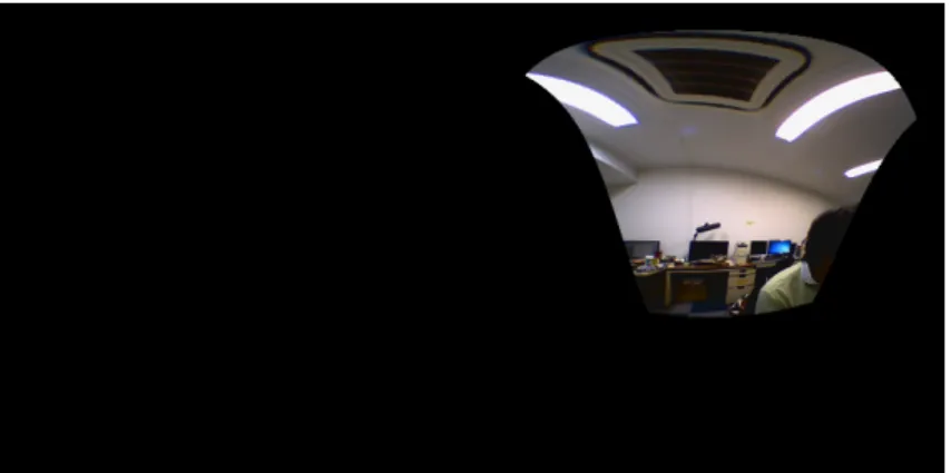
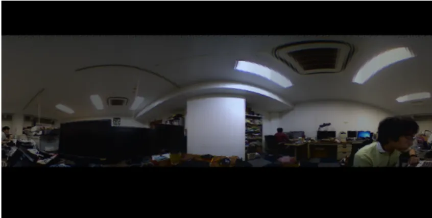
A single RGB image warped to an equirectangular image is shown in Fig. 3.12. Map-ping all RGB images similary and smoothly blending them gives us Fig. 3.13. These images are typical results of operating the scanner on a desk in a room.

(28)

Figure 3.11: Equirectangular projection of spherical coordinates.

Figure 3.12: A single RGB image warped to equirectangular coordinates.

equirectangular image I can be calculated by smoothly blending the images using Gaus-sian weight function with the following formula.

I(θ, ϕ) = ∑ i_∑Ii(θ, ϕ)wi(ϕ) iwi(ϕ) (3.1) wi(ϕ) = exp ( −(ϕ− ϕi)2 σ2 ) (3.2) where ϕi is the center of scan i. σ is a blending constant and set to approximately 2.5◦ (half of the capturing interval).

Notice there are several bands of diﬀerent color and brightness in Fig. 3.13. These artifacts are caused by auto exposure (AE) and auto white balance (AWB) of the RGB camera. We negate AE and AWB by calculating color multiplier αi for each RGB image, and then applying multiplication before merging images. The multipliers are calculated to equalize average colors of neighboring images in the overlap region. The overlap region is approximated by weighting function wij(ϕ) = wi(ϕ)wj(ϕ). Using this function, multipliers can be calculated as solution of Eq. (3.3).

(29)

Figure 3.13: Stitched RGB image. αi ∑ θ,ϕ wij(ϕ)Ii(θ, ϕ) = αj ∑ θ,ϕ wij(ϕ)Ij(θ, ϕ) (3.3)

Also, we have a normalization Πiαi = 1. These equations form an over-constrained system, but the solution generally exists in practice.

The merged image after color correction is shown in Fig. 3.14.

Figure 3.14: Stitched RGB image with color correction.

Notice the seams between bands are almost invisible. We also apply vignetting removal using naive cos4 _{model[30] to RGB images before merging.}

3.2.3 Distance Image Noise Removal and Point Cloud

Genera-tion

Equirectangular images are suitable for preserving topology of neighboring pixels, but are unsuitable for operations such as 3D plane ﬁtting which is required for ceiling detec-tion. Another problem of using an equirectangular distance image for 3D processing is

(30)

that resampling of the distance is required for virtually any operation, including transla-tion and rotatransla-tion. Resampling of the LRF distance is carefully avoided in the proposed system, because resampling causes artifacts regardless of interpolation method. Fig. 3.15 shows an original data, and results containing artifacts when resampled at triple reso-lution with linear interpolation and no interpolation (i.e. nearest neighbor lookup). A pertinent format is a point cloud with colors and normals, which can be represented as a set of (point, color, normal). In this section, however, we extensively use resampled equirectangular images for visualization purpose.

Figure 3.15: Resampling artifacts of distance images.

The raw LRF data contains distance noise of a few centimeter, which is prohibitively large for computing normals from adjacent points. Fig. 3.16 shows an example of point cloud generated without noise reduction. Thus, it is necessary to reduce the noise in distance data.

Normals of each point is calculated as a cross product of tangent vectors. The distances and positions of the points are stored in 2D arrays without any resampling.

N (x, y) = ∂P (x, y)/∂x× ∂P (x, y)/∂y

∥∂P (x, y)/∂x × ∂P (x, y)/∂y∥ (3.4) where N (x, y) is normal, and P (x, y) is 3D position at pixel (x, y). P can be calculated from distance image D by multiplying distance and a unit direction vector calculated from spherical coordinates (θ, ϕ). Fig. 3.17 shows an example of D. Although D looks smooth visually, calculating normals from derivatives ampliﬁes the noise, resulting in unusable

(31)

Figure 3.16: A view of a ﬂat region in a point cloud, showing errors of a few centimeters. The ﬂat region is highlighted in orange.

normals shown in Fig. 3.18.

Figure 3.17: Distance image D. Pixel brightness is proportional to distance. A naive Gaussian blurring of distance images will reduce the noise, but it will also blur the edges. We uses a trilateral filter[31] to blur distance image while keeping edges relatively intact. While a Gaussian blurring filter takes only one image and blurs it, a trilateral filter takes one additional image for edge information extraction purpose.

However, we cannot get edge information from distance image, because D is continuous at edges, and only its derivatives are discontinuous, which is noisy when numerically computed. The RGB image is good in theory, because the amount of light reflected by a surface is heavily influenced by the surface normal. However, the RGB image has offset error of a few pixels relative to LRF images, making it unsuitable. Fortunately, the LRF outputs reflected infrared intensity image R, which is shown in Fig. 3.19.

Since the LRF scans by emitting laser and measuring its reflection, the reflected in-tensity image R is equivalent to an infrared photo taken at the position of the LRF, with a single infrared point light also at the LRF position illuminating the whole scene. The intensity image contains edge in a clearer way, so R is used at the input of trilateral filtering. A normal image N computed from denoised D is shown in Fig. 3.20.

(32)

Figure 3.18: Normals calculated from raw distance image. (XYZ components are visual-ized as RGB color.)

Figure 3.19: Intensity of reﬂected infrared light.

preserved without getting blurred. The empirically found optimal parameters for the tri-lateral ﬁltering are 3 px, 0.2 m, 100, when the range of the intensity values is [0, 215_{] (which} is speciﬁc to the model of the LRF used in the scanner). Finally, P and N are converted to a point cloud, and the points are colored by looking up the RGB equirectangular image. Fig. 3.21 shows a point cloud obtained by scanning a room from a single location.

3.3 Indoor Environment Reconstruction Method

3.3.1 Overview

In indoor reconstruction step, scene model is generated from 3D scan data. However, as discussed in section 2.4, scene reconstruction is a very hard problem and various com-promises are necessary, some of which forms a certain trade-off. The trade-off is between accuracy (i.e. conformity of generated scene model to input data), and realness (i.e. per-ceived probability of generated scene model occurring in reality). Note that this trade-off is different from the trade-off between cost and realness discussed in subsection 3.1.1. The proposed indoor environment reconstruction method always favors realness to accuracy, because the goal of the system is to trigger fear via realness. The overall dataflow of the reconstruction method is shown in Fig. 3.22.

(33)

Figure 3.20: Normals calculated from ﬁltered raw distance image.

Figure 3.21: A point cloud generated from 3D scan data at a single location. Initially, the system does not have locations of the scanner at the times of scanning. These locations, or poses, are calculated by aligning 3D scan data into a single point cloud. However, the merged point cloud contains ghosting artifact due to alignment error and scan distortion. So the merged point cloud is only used to extract a room frame, which represents overall room shape as an extruded polygon. The extruded polygon is equivalent to a pair of 2D floor map and room height. When calculating the room frame, Manhattan world assumption[32] is used as a hint to make a room frame visually pleasant. Under Manhattan world assumption, all surfaces in a scene are flat and their normals are parallel to either X, Y or Z axis. Although this holds true for many man-made objects, the proposed method does not strictly rely on it because there are also a significant number of exceptions.

Computation after the room frame extraction is based on either individual point clouds and equirectangular images, as they do not suﬀer from ghosting artifact. The remaining process can be divided into three independent processes of light detection, boundary generation and object extraction.

In the ceiling light detection process, lights in the room are detected from an equirect-angular image. Lights are required for generating dynamic shadows when objects move in an earthquake. In the boundary generation process, texture of the room is calculated

(34)

Figure 3.22: Dataﬂow of indoor reconstruction pipeline.

from an equirectangular image, and then the missing part of the texture occluded by objects are inpainted. In the object extraction process, points corresponding to interior boundary (such as walls) are removed using the room frame, and the remaining point clouds are divided into small patches by geometrical proximity. Since each patch is a subset of the point clouds, a patch itself is also a point cloud. A patch typically repre-sents an incomplete surface within a single object. Then, the patches are linked together to form physically stable clusters. A cluster is a set of patches, and it corresponds to a single object detected by the system. Finally, appearance and physical models of objects are created from the clusters.

Finally, the boundary, the objects and the lights are combined to form a complete scene model.

(35)

3.3.2 Alignment of 3D Scan Data

The 3D scan data comprises of equirectangular images and point clouds taken from multiple locations. To detect objects in the scene, the system needs to recover the relative locations of the point clouds, which are arbitrary chosen by the operator to maximize a coverage of the scanned room. The process of estimating the locations and forming a single merged point cloud is called alignment.

The alignment is known as a hard problem in a general case. Although several meth-ods[33][34] are known, their accuracy is mostly unpredictable. In the proposed system, a typical property of an indoor room, specifically presence of a flat ceiling, is exploited. Unlike walls and floors which are often occluded by objects, a ceiling can be observed with high probability by the scanner, making it suitable to use as a feature to partially align point clouds.

First, point clouds are partially aligned by using the ceiling as a feature observable in all scan data. After ceiling alignment, the point clouds are constrained to translation and rotation on a 2D plane, leaving only 3 degrees of freedom (DoF). Second, a novel pose-invariant similarity measure is used to associate the point clouds by similarity. This results in a pose tree, from which relative poses of point clouds can be uniquely determined. Finally, a pairwise ﬁne alignment method called iterative closest point (ICP)[35] is applied to the pose tree, and ﬁnely aligned relative poses are calculated from the pose tree.

Partial Alignment using Ceiling as a Feature

When the scanner is used, it is placed on a nearly level surface in a location accessible to a human. In conjunction with the fact that the scanner is nearly omnidirectional, there is a high chance that each scan data contains the ceiling. Thus, the ceiling can be used as a feature to align the point clouds partially.

In a scan data, the ceiling forms a nearly level plane because of the ceiling. To detect this plane, RANdom SAmple Consensus (RANSAC)[36] is applied to ceiling candidate points PC. PC is calculated as follows from the point cloud P , assuming Z+ corresponds to up direction.

PC ={p | p ∈ P, pz > (max p′∈P p

′

z)− kmargin} (3.5) where pz is the z coordinate of point p. kmargin is empirically set to 50 cm, so that other large planes such as desks will be rejected, while ensuring to retain the points originating from the true ceiling even in the presence of recessed ceiling decoration.

Point clouds are rotated and translated so that the detected planes become completely coplanar. After this, we only need to consider 2 translational DoFs and 1 rotational DoF

(36)

in a plane when trying to align the point clouds completely.

Pose-invariant Similarity Measure

First, a non pose-invariant similarity measure is deﬁned, and then a pose-invariant similarity measure is derived from it assuming the points clouds are partially aligned by the ceiling feature.

The (non pose-invariant) distance d between two point clouds P1, P2 is deﬁned using Eq. (3.6). The distance d is a similarity measure, calculated by ﬁrst binning the points into voxels (cells of 3D lattice), and then comparing average colors and normals in each voxel. d(P1, P2) = 1 M ∑ i∈ Z3 if |V (P1,i)|>0 and |V (P2,i)|>0

knN (V (P1, i))· N(V (P2, i)) + kc∥C(V (P1, i))− C(V (P2, i))∥

(3.6) N (P ) = ∑ p∈P(pxpypz)⊤ ∥∑p∈P(pxpypz)⊤∥ (3.7) C(P ) = 1 |P | ∑ p∈P (prpgpb)⊤ (3.8) V (P, (i, j, k)) ={p | p ∈ P, ⌊px/s⌋ = i, ⌊py/s⌋ = j, ⌊pz/s⌋ = k} (3.9) where M is a number of voxels which contain one or more points from both P1 and P2, s is a size of voxel, and kn and kc are weights of normal similarity and color similarity. The weights and the voxel size are empirically set to kn= 5, kc= 0.01, and s = 15 cm so that d can distinguish diﬀerent point clouds while not being too sensitive to noise in color and normal.

To create a pose-invariant similarity measure, we need to cancel the eﬀect of translation and rotation on the measure. Basically, multiple variations of a point cloud are created, and each variation is compared to the other point cloud using d. By creating enough variations, one of the variations would correctly align. Thus, using the minimum of d as a measure, a new pose-invartiant measure dinv can be deﬁned.

First, function E that creates variants of a point cloud by rotation, is deﬁned. Also, let A be a function that translates a point cloud so that the center coincides with the origin.

E(P ) ={Rz(2πk krot

)P | k ∈ {1, 2, . . . , krot}} (3.10)

(37)

where center(P ) is the center of axis-aligned bounding box of P , Rz(θ) is rotation along Z axis by angle θ, and krot is a constant specifying number of generated variants. When krot is smaller, fewer variants are generated and the computation is faster. However, krot also needs to be large enough so that the diﬀerence of rotation angles between the point clouds (P1, P2 in Eq. (3.12)) becomes small enough for the later ﬁne alignment to converge correctly. Empirically, krot = 60 is found to satisfy both conditions.

In most case, the center of a scan data is the same as the center of the whole room, due to the omnidirectional nature of the scanner. Thus, the center of a point cloud can be used a reliable feature to normalize the translation of point clouds in A. Note that there is a subtle difference in calculating the center in a partially aligned point cloud, and detecting the walls in a unaligned point cloud. The former is significantly more reliable than the latter, because only a single point is enough to calculate the center correctly, but a significant portion of the walls must be observed for direct wall detection.

Unlike translation, rotation cannot be normalized by a simple feature like center of the point cloud. Thus, E samples uniformly from all possible rotations. By combining A and E, the pose-invariant distance dinv of two point clouds can be deﬁned like Eq. (3.12). By keeping track of which variation minimizes dinv, a transform Ti→j that transforms Pi to Pj can be recovered. Accuracy of Ti→j, however, can be aﬀected by various factors, such as an amount of noise and how well assumptions (e.g. ceiling feature) hold.

dinv(P1, P2) = min P₂′ ∈ E(P2)

d(A(P1), A(P2′)) (3.12)

Construction of Pose Tree

By using the pose-invariant distance measure dinv, point clouds can be paired against similar point clouds. For all pairs of point clouds, dinv is calculated. The result can be expressed as a symmetric matrix, which is shown in Fig. 3.23. The matrix can be also seen as a graph, whose node is a point cloud and edge is dinv, as shown in the left of Fig. 3.24.

To calculate relative pose Ti→j between Pi and Pj, each transforms on the path need to be multiplied. However, since there are multiple possible paths between nodes in a graph and the transforms are inexact, diﬀerent paths would result in diﬀerent relative poses. To uniquely determine relative poses of all point cloud, only one path should exist between any two nodes, as shown in the right of Fig. 3.24. In other words, we need to form a spanning tree of the graph, which we call a pose tree. Also, the sum of dinv in a spanning tree should be minimized, because transforms between similar point clouds (i.e. smaller dinv) have higher chance of being accurate. A pose tree with minimum sum of dinv can be calculated by applying Prim’s algorithm[37] to the graph. An example of obtained

(38)

Figure 3.23: dinv for all point cloud pairs.

Figure 3.24: Multiple paths from a node to another in a graph (left). There is only single path between nodes in a tree (right).

pose tree is shown in Fig. 3.25.

Recovering Poses from Pose Tree

Although the pose tree provides a way to uniquely determine the relative poses, trans-forms corresponding to edges of the pose tree have accuracy only up to voxel size s. To obtain the fine relative pose, each edge is finely aligned by a variant of ICP method im-plemented in point cloud library[38]. An ICP method takes two coarsely aligned point clouds, and aligns them by iteratively minimizing distance between points like gradient descent. The ICP method is applied to all edges of the pose tree, and now finely aligned relative poses can be obtained from the pose tree in the same way coarse relative poses are obtained. We can also merge the all point clouds into a single point cloud by using the fine relative pose. After the alignment is complete, all point clouds are merged into a single point cloud.

Although the alignment is automatic, some scan data could converge to a wrong pose, in which case a manual adjustment is needed.

(39)

Figure 3.25: A minimum spanning tree of the point clouds. Each node is a point cloud, and each edge is dinv between two point clouds.

3.3.3 Room Frame Extraction

The reconstruction target of the system is an enclosed room, whose walls and ceiling are mostly ﬂat. Although point clouds and equirectangular images contain all information obtained by the scanner, it is useful to have an intermediate representation of the room shape, which is called a room frame in this thesis. A room frame is used in subsequent processes such as light detection and object reconstruction. In room frame extraction process, Manhattan world assumption[32] is partially enforced to reduce the noise and to produce more visually pleasant and less computationally demanding results.

Both scan data and a room frame are represented in 3D Cartesian coordinates whose Z axis represents the vertical direction. A room frame represents the shape of a room as an extruded polygon. Thus, a room frame is a composition of 2D polygon in XY coordinates and two values to specify the range of the room on Z axis.

A merged point cloud is projected onto the XY plane, and the resulting 2D points are used to calculate the 2D polygon. An example of projected points is shown in Fig. 3.26. In Fig. 3.26, it can be observed that the region corresponding to inside of the room is very dense, and the outliers are relatively sparse. Upon close inspection of the point cloud, outliers typically originate from exterior scene captured through transparent windows, or from interior scene reﬂected by windows or other mirror-like objects.

Prior to 2D polygon estimation, the projected points are filtered by a 2D voxel filter of 10 cm. The voxel filter replaces the points in a given voxel with the average of the points.

(40)

Figure 3.26: 2D projection of a merged point cloud, consisting of 4,065,020 points. In this 7 m_{× 4 m oﬃce, 15 scan data were taken.}

By the ﬁltering, point density is equalized across the space, and most of the outliers are decimated as shown in Fig. 3.27.

Figure 3.27: 2D Points after ﬁltering.

Then, a concave hull is calculated from the filtered points. Unlike the convex hull, the concave hull is ill-defined and the results depends on a selection of a method and its parameters. For room frame extraction, concave hull extraction method by Moreira et al.[39] is used. The method takes an extreme point in a direction as the input, and a concave hull containing larger density region is carved out from the starting point. Since the outliers are highly decimated by the filtering, the method would obtain a convex hull corresponding the room shape, if given a correct starting point.

This is achieved with a rejection sampling method with the following steps. First, the extreme point in a randomly chosen direction is chosen as the starting point. Then, the resulting concave hull is accepted as correct if it is large enough in area, and not too narrow. More concretely, it will be rejected if it spans less than 1 m in any direction. Otherwise, it is rejected and a new starting point is chosen. These steps are repeated until an acceptable solution is found. A result of the process is shown in Fig. 3.28.

(41)

Figure 3.28: A concave hull extracted from a ﬁltered points.

are two issues that prevent using the shape as the 2D polygon of the room frame. First, the shape is too noisy. In particular, false unevenness in flat regions and slightly off right angles would result in visually unpleasant and unnatural look, as shown in Fig. 3.29. Second, there are too many vertices in the shape to allow efficient querying such as inside/outside test. However, it is problematic to enforce the Manhattan world assumption completely, because it will obscure the chamfered edges at the corners of the room. The presence of chamfered or rounded corners is not limited to the example, but they are also common in a typical indoor environment.

Figure 3.29: Vertical bands on a ﬂat region, caused by noisy normals.

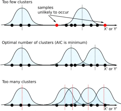
Manhattan world assumption is partially enforced by forming a non-uniform grid, and then snapping vertices to the grid. First, a histogram of the edge normals is calculated, and the principle axes X′ and Y′ are estimated from its mode. Then, a non-uniform structured grid is formed by clustering the X′ and Y′ elements of the vertices independently.

To this end, the k-means method is used. The k-means method is a clustering method, that can detect k groups of concentrated samples. Typically, k must be speciﬁed manu-ally, but in the proposed method, k is automatically determined by minimizing Akaike Information Criterion (AIC)[40]. The values can be though of as being sampled from unknown true values with a certain error distribution. Intuitively, AIC can ﬁnd an ap-propriate balance between likelihood of samples and information required to represent the