Three Criteria for Selecting Variables in the Construction of Near-Optimal Decision Trees

238

Three Criteria for Selecting Variables

in the

Construction

of Near-Optimal Decision Trees

Masahiro MIYAKAWA and

Nobuyuki

OTSU

(宮川正弘)

(

大津展之

)

Electrotechnical

Laboratory

1-1-4 Umezono, Tsukuba, Japan 305

Abstract

Forconvertinga decision table toa near-optimal

deci-sion tree in thesense ofthe minimal number ofnodes

of the tree, wepropose threecriteriafor variable

selec-tion: $\Gamma_{A},$ $\Gamma_{H}$ and $\Gamma_{D}$ from three different standpoints

of combinatorial, entropy and discriminant analyses.

First we examine “static“ behaviors of the criteria,

e.g. rejection of nonessential variables (nev-free), se-lection of a totally essential variable (tev-bound) and

selection of a quasi-decisive variable (qdv-bound). It

is shown that $\Gamma_{A}$ is nev-free, tev-bound but not $qdv-$

bound, while$\Gamma_{H}$ and$\Gamma_{D}$ have the complemental

prop-erties. An experiment to evaluate the performance of

the criteriashows that each ofthe criteria gives good

near-optimum trees, indicating that $\Gamma_{D}$ and $\Gamma_{H}$ are

practically comparative and $\Gamma_{A}$ is slightly better. All

the criteria require at most $O(L^{2}2^{L})$ operations with

$O(L2^{L})$ storage, where$L$ is thenumber ofvariablesof

the input table.

1.

Introduction

A decision tableisalist of“rules“. A rule consistsof a

pair of“logical conditions“ andan “action” which

spec-ifies the action tobe executed when the conditions are

satisfied. Taking Boolean values for both conditions

and actions, it represents a Boolean function; taking

feature vectors for conditions and object

names

for

ac-tions, it gives a description of a pattern. The

occur-rence ofa decision table is rather wide. Identffication

ofa specimenin biologicalscience is apractical

exam-ple ofdecision table. Ifwecountits useas aconceptual

tool, then it appearance is even wider. For example,

a typical situation in knowledge engineering or even

a program, e.g. so called Janov scheme, can also be

schematized in decision tableterms. An important

fea-ture of a decision tableis that it specffies only avery

restricted part oflogical possibilities and leaves the

re-mainingpart as “don’t cares” orunconcerned(inother

wordsmost decision tables specify part\’ial functions).

In a typical use of a decision table to identify an

unknown “input object”, one tests each single property

in sequence until the object is determined uniquely.

This procedure is called a sequential test procedure and

isconveniently representedby a decision tree $[ReS67]$.

In most practical cases a decision may be made by

testingonly some ofthe properties. In addition there

are fairly large tables (e.g. having dozens number of

properties) whichareunable to be manually converted

intoefficient trees. Thus an automatic conversionof a

table into an optimum or near-optimum tree is most

desirable [MTG81] and the central problem being to

determine the order oftesting of the properties.

It is known that the construction problems of

vari-ous optimum decision trees are NP-complete $[HyR76$,

Mor82] when agiven input table is not in ”expanded”

form (most frequent in practice as we mentioned

be-fore). Several heuristicsofconstructing near-optimum

treeshave been proposed; mostly fortreatingthe don’t

care entries (cf. [Ver72]). Given an L-variable

ta-ble, one can construct an optimum,

i.e.

a

minimum-cost tree by applying a dynamic programuning

tech-nique which always requires $O(L3^{L})$ operations

(com-parisons) with $O(3^{L})$ storage [Bay73, $ScS76$]. On the

other hand, a simple top-down heuristic method

em-ploying asuccessivevariableselection, viz. VSM

(vari-able selection method) can construct a near-optimum

treeinfarless operations if an efficient selection is

guar-anteed. Moreover, it hasan advantage of applicability

to amost practical caseof partial functions.

In this paper we adopt the number ofinternal nodes

of a tree as a cost of a tree (i.e. as an optimality

cri-terion) and propose three criteria for the VSM: $\Gamma_{A}$

from the combinatorial standpoint, $\Gamma_{H}$ from the

en-tropy standpoint and $\Gamma_{D}$ from the discriminant

anal-ysis standpoint. Naturallywe want to determine their

performance comparing with optimalone and also the

数理解析研究所講究録 第 731 巻 1990 年 238-249

239

best heuristic among the three. Can we prove this by

some

means? As a first approach we investigate their

behaviors

in typical situations, namely we check

rejec-tion ofnonessential variables (nev-free) and selection

ofa totally essential variable or a quasi-decisive

vari-able (tev- or qdv-bound). Note that $nev$ is a worst

variablewhile $tev$ and $qdv$ are optimal ones. We show

that $\Gamma_{A}$ is nev-free andtev-boundbutnot qdv-bound,

while $\Gamma_{H}$ and $\Gamma_{D}$ have just the complement

proper-ties. Thus, as a next step, this leads us to conduct

an experiment research to compare the performance.

It shows that the criteria actually give near optimum

trees. Also the performance of$\Gamma_{D}$ and $\Gamma_{H}$ practically

coincides (1.05 intheaveragecompared with optimum

one) and $\Gamma_{A}$ is slightly better (1.03 by the previous

measure). All the criteria require at most $O(L^{2}2^{L})$

operations (bit-comparisonsor integer-additions)with

$O(L2^{L})$ storage (this is apolynomial bound ifwetake $2^{L}$ size of an expanded table intoaccount).

The construction ofa tree having a minimum

num-ber ofnodes has been received less attention to

com-pared with that of a tree having a minimum average

path lengths [Gar72, $MiS80$, MTG81, Miy85].

How-ever, the minimum cost is an invariance of the table,

representingtheminimumnumberof“dividing” of the

table necessary to decomposeit intoconstanttables; a

quantity inherently related to a complexity of the table

[Bud85, Lov85, Weg84]. This problem is also directly

related to the design of PLA (programmable logic

ar-ray) in which itis important to obtain complement of

a logical function in the form of asfew product terms

as possible [Cha87, Sas85].

2.

Definitions and

Preliminaries

Let us denote $L$ properties simply by numbers

$\{1, \ldots, L\}$

.

Let $\{a_{1}, \ldots, a_{K}\}$ be the set of$K$ actions.

Assume that each property $i$ takes, for simplicity, the

binary value $x_{j}=0$ or 1. We are given a

map-ping $f$ : $\{0,1\}^{L}arrow\{a_{1}, \ldots, a_{K}\}$, called an $L- ary$

-K-action decision table, or simply a table, which maps

the values of the properties into the actions. Let $x=$

$(x_{1}\cdots x_{L})\in\{0,1\}^{L}$

.

A pair $(x, f(x))$ is called a $nAle$

.

Often we denote a rule simply by a vector $z$ since it

uniquely determines a rule. We treat a table $f$ as the

set of all $2^{L}$ rules. InTable 1 we give an example of a

table in reduced form (a) and in expanded form (b).

2.1.

Subtables and

fixations

Given an initial table $f$, a subtableis arestriction

$f(x_{1} . . . x_{i_{1}-1}s_{1}x_{i_{1}+1}\ldots x_{i_{h}-1}\ldots s_{h}x_{i_{h}+1}\ldots x_{L})$

$=$ $f|$($x_{\dot{*}m}=s_{m}$ for $m=1,$$\ldots,$ $h$)

Table 1: A decision table: (a) reduced form, (b)

ex-pandedform.

which is an $(L-h)$-ary function. The variables

$x_{i_{m}},$ $m=1,$$\ldots h$) $’ 0\leq h\leq L$ are called

fixed

(to $s_{m}$; $s_{m}=0$or 1), and theremaining variablesare

free.

A subtable consistsof all vectorssome (say h) of their

elements equal fixed constants. The number $L-h$ of

freevariablesis the arity of the subtable. Sometimes it

is convenient to show it explicitly like $L-h$-subtable

(thustheinitial tableis an L-subtable while a rule is a

O-subtable). Since the initial table consistsof$2^{L}$ rules,

we have $2^{2^{L}}$

different subsets, among them $3^{L}$ subsets

are subtables.

The sole type of restrictions $f|(x_{i_{m}}=s_{m}$ for $1\leq$

$m\leq h)$ we deal with is called a

fixation of

$f$and

de-noted by $fi_{1^{1}}^{s}\cdots i_{h}^{s_{h}}$ orsimply $f\alpha$, where $\alpha$ denotes a

catenation $i_{1}^{s_{1}}\cdots i_{h^{h}}^{s}$. The null fixation $\lambda$ corresponds

to theinitial table$f$

.

Thisnotationconveniently

repre-sents the successive generation ofsubtables in the tree

by means of “dividing“ of a table, which is described

below.

2.2.

Decision

trees

and

Variable

Selec-tion

Method (VSM)

A decision tree [Miy85] for$f$isa binarytree associated

with each internalnode two objects: a subtable and a

variable (called a test variable), and with each leaf a

decision action according to the following algorithm:

If$f$ is a constant (i.e. $f$ consists ofasingle action)

then the decision tree for $f$ issimply asingle leafwith

the decision action. Otherwise it is a tree with a root

associated with the subtable $f$ and with any its free

variable$i$as the test variable,havingtheleft andright

subtrees corresponding to the subtables $fi^{0}$ and $fi^{1}$,

respectively (theedges leading to them are labeled by

$0$ and 1, respectively).

Thuseverytree we deal with

is

an extended binary

in-240

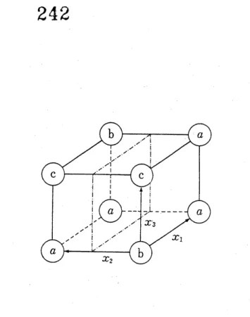
Figure 1: Dividing a table$f$ by avariable $i$. Figure 2: Example trees: (a) non-optimal. (b) optimal.

edge (except the root $R$ which has no in-edge) and

either zero or two out-edges. External nodes (leaves)

arethose withnoout-edges. Theremaining nodes are

called intemal. We call a decision tree simply a tree.

One maythink that each rule $x$ of a table $f$is

iden-tified as belonging to $fi^{0}$ or $fi^{1}$ according to $x;=0$

or 1, respectively, at each internal nodewhere the test

variable$i$is located. A path of the tree represents

suc-cessive such fixations. Thus a tree can be considered

as a device to determine values of a givenfunction by

means ofsuccessivefixations. We denote a tree by$T$,

or$T[f]$whenit isnecessary to indicate the initial table.

Given a criterion to choose a test variable, one can

construct a treebyconsistentlyselecting test variables

according to the criterion. This general algorithm

for constructing a tree is called a Variable Selection

Method (VSM). Thebasic operation ofmaking

L–l-subtables $fi^{0}$ and $fi^{1}$ from $f$ is called (dividing’ ofa

table (this correspondstorefining the action set inthe

table).

A VSM ends in $O(2^{L})$ operations, since possible

number ofsuch dividing of atable is at most$2^{L}-1$

.

2.3.

Minimum decision trees

For an L-ary table $f$, therecan be at most $\prod_{:}^{L_{=1}}i^{2^{-1}}$

equivalent trees $[ScS76]$. To construct “efficient” trees

we adopt the number ofinternal nodes ofatree $T$as

a cost of a tree and denote it by $|T|$

.

Since no test is

required at leaves, $|T|$ is the cost forrepresenting the

whole test procedures of$T$, assumingthat the

determi-nation ofthe value of each property incurs a uniform

cost. We call a tree minimum(optimum) whenits cost

is aminimum

among

alltrees corresponding tothe

ta-ble $f$

.

In

Fig.2

we

indicate

a tree and a minimum tree

for the table of Table 1.

2.4.

Nonessential,

totally

essential

and

quasi-decisive variables

Beforegoingtovariable selection criteria, we introduce

some notions concerning “good” variables. To do this

we need a notation to represent fixed and free

vari-ables of a subtable. Our discussion usually concerns

an arbitrarily fixedsubtable $f$and itsdirect subtables

$fi^{s}$ for $s=0,1$

.

Let $f$ have all $h$ variables denoted

by 1, .

..

,$h-1$ and $j(i\neq j, i=1, \ldots, h-1)$

.

Let

$u=u(1)\ldots u(h-1),$ $u(i)=i,$ $i=1,$$\ldots$,$h-1$ denote a

sequence (i.e. catenation) ofvariables 1,.

. .

,$h-1$

.

Let

$x=x(1)\ldots x(h-1),$ $x(i)=0$ or 1 for $i=1,$$\ldots,$$h-1$,

denote a bit sequence of length $h-1$

_.

Let us

abbrevi-ate a fixation $u(1)^{x(1)}\ldots u(h-1)^{x(h-1)}$ by$u^{x}$ for

sim-plicity. Now, let $u^{x}j$ represent a vector in which the

variables in $u$ are fixed to the values $x$ and avariable

$j$ is free. Finally, let us denote a l-subtable called a

j-parr by $f(u^{x}j)\equiv fu^{x}(u^{x}j)$, which consists of a pair

of rules of $f:(u^{x}j^{0}, f(u^{x}j^{0}))$ and $(u^{x}j^{1}, f(u^{x}j^{1}))$

.

If

twoactionsof aj-pair coincide, it is a constantj-pair,

otherwise it is a nonconstant j-pair. Each fixation $u^{x}$

which gives constant or nonconstant j-pair is called

inactive or active fixation for$j$, respectively (hereafter

only $x$ is indicated instead of$u^{x}$ since _$u$is determined

as the (complement’ sequence of$j$).

Example 2.1. For $x=10$ and $u=23$ thefixation $u^{x}$

denotes $2^{1}3^{0}$. Then l-pair _{$f(2^{1}3^{0}1)=f2^{1}3^{0}(2^{1}3^{0}1)$}

in Table 2.1 is a constant l-pair, while $f(2^{0}3^{0}1)=$

$f2^{0}3^{0}(2^{0}3^{0}1)$ is a nonconstant l-pair. Hence the

fix-ation$2^{0}3^{0}$ is activewhile $2^{1}3^{0}$ is inactive.

A variable $i$ is nonessential in $f$ ifeach fixation $x$

for $i$ is inactive, i.e. _{$f(u^{x}i)=a_{j}$} for each _$x$ (a

con-stant action

$a_{j}$ depends

on

$x$). Also,

a variable

$i$

is

$24i$

$f(u^{x}i)\neq$ const. for each $x$

.

When all variables are

nonessential

then $f$ is a constant. Nonessential

vari-able and totally essential variable are abbreviated to

$nev$ and $tev$, respectively. A minimum tree doesn’t

have nevs as test variables [15]. A $tevi$ is an

opti-mum

variable [6], that is, the tree becomes minimum

if we choose $i$ as a test variable and make its left and

right subtrees minimumfor $fi^{0}$ and $fi^{1}$, respectively.

Note that there cpuld be acase that someof the rules

are never executedactually (e.g. they could beimplied

byothersinpractical tables; this can be handledby

as-signing “probability” $0$to them). Theneven “essential

variables” need not be tested at all inthe tree. So in

this case the notion of “essentiality” should be

modi-fiedin an appropriate way. Throughout this paper we

assumethateach ruleisexecutable,i.e. the probability

of each rule is not $0$

.

There is another optimal variable. A variable $i$ is

decisive if$fi^{0}=a$ (cost.), $fi^{1}=b$ (const.) and$a\neq b$

.

A variable $i$ is quasi-decisive (abbreviated to _$qdv$), if

$fi^{s}=$ const. and $fi^{i}\neq$ const. for strictly either one

of $s=0$ or 1 [14]. A $qdv$ is an optimalvariable with

respectthe cost definedinthis paper (however,itis not

an optimal variablein general with respect to another

one (e-cost)) [14].

Therefore,itis desirable fora criteriontoreject nevs

and select a $tev$ or a $qdv$ whenever they exist. Let us

callacriterion

_nev-free

ifitselects nonevs. Again, let

us call acriterion tev-bound or qdv-bound if it selects a

$tev$ or a$qdv$ whenever they exists.

In the next section we propose three VSM criteria

andexamineabovepropertiesfor them. Thisis

impor-tant for understanding the performanceofthe criteria,

since it is extremely difficult to show something

for-mallyabout the performance of thiskind ofheuristics.

3. Three

criteria

for

variable

se-lection

Weshall introduce three criteriafor variable selection

to construct an efficient tree in the sense of minimal

number of internal nodes (i.e. dividing). Our basic

strategy is to “produce constant tables as fast as

pos-sible“,sinceno moredividingis necessaryfor constant

tables. To do thiswe introducethreemeasuresof$(dis-$

tance” between a table and a constant from three

dif-ferent standpoints. Thenour criteriasimplyselectsuch

$i$that the “distance” between_$fi$“ and a constant

func-tionfor both $s=0$ and 1 become a

minimum

among

allvariables.

The first criterion $\Gamma_{A}$ is implicit in some literature

$[23,19]$, approaching the problem from

combinatorial

analysis. The second criterion $\Gamma_{H}$ is presented in

[7,13,17]. Also there are several literature inwhich the

notion of entropy is applied for the problem in other

context (mostly with the treatment of “don’t care“

symbols $(-$“$)$ [6]. The entropy approach “views” the

occurrences of the actions as stochastic events. The

third criterion $\Gamma_{D}$ is new [13] and from the

discrimi-nant analysis standpoint [4], which is related to

multi-variate data analysis. In this framework, we use the

notion of((

$mean$ value” of the variable$x$; with respect

to the action $a_{j}$ (denoted by $\mu_{j}^{\dot{*}}$) as well as the total

mean value (denoted by $\mu_{T}^{:}$ whose valueis always 1/2

since wehave thesame number of ruleshaving $x;=0$

and $x;=1$), treating the values $0$and 1 as real

num-bers.

Before giving a detailed explanation of the criteria,

wegive notations and equations. We denoteby $N_{j}$ the

number of theoccurrencesof the action$a_{j}$ in$f$, by$N_{j}^{i}$

thenumber of rules $(x, f(x))$ suchthat $f(x)=a_{j}$ and

$x_{i}=s$for$s=0,1$

.

Further, let class$(j)$denote the set

of vectors corresponding to action $a_{j}$

.

There hold the

followingequations. 1) $N_{j}^{1^{O}}+N_{j}^{*^{1}}=N_{j}$, 2) $\sum_{j}N_{j}:=N^{i}=2^{L-1}=N/2,$ $s=0,1$, $3) \sum_{i}jN_{j}=N=2^{L}$, 4) $p_{j}$ $:=N_{j^{1}}/N^{i}=2N_{j}^{i}/N,$ $s=0,1$, 5) $w_{j}$ $:=N_{j}/N,$ $\sum_{j}w_{j}=1$,

6) $\mu_{j}^{1}$ $:=E_{j}x:= \sum_{class(j)}x_{i}/N_{j}=N_{j}^{i^{1}}/N_{j}$,

7) $\mu_{T}^{:}$ $:=Ex;= \sum x_{i}/N=\sum_{j}N_{i}^{1^{1}}/N=1/2$;

$\mu_{T}^{i}=\sum_{j}w_{j}\mu_{j}^{i}$

.

Now we present the threecriteriatogether withtheir

ranges forall tables.

Activity

criterion

$\Gamma_{A}$

.

Define$A$; tobethenumber

ofactive i-pairsof$f$

.

Anactivei-paircanbeconsidered

as alogical unit tobe separated bydividinga table (cf.

Fig 3). Then $A;= \sum_{:}^{n}A_{i}$ represents the total number

of i-pairs of $f$

.

Since $A_{2}$ active i-pairs disappear by

dividing $f$ by $i$, we select a variable $i$ which have a

maximumnumber of$A$; among all variables.

Lemma 3.1. The number

of

active i-pair$A$

:

ranges

$0\leq A;\leq 2^{L-1}$

.

The best value $A_{i}=2^{L-1}$ is attained

if

and only

_if

$i$ is a totally essentialvariable

of

$f$, and

theworst value $A_{i}=0$

if

and only

if

$i$ isa nonessential

variable

_of

$f$

.

Proof.

Obvious fromthe definition. $\square$

Entropy

criterion

$\Gamma_{H}$

.

The actions

$a_{j}$

in

a

ta-ble$f$ can be considered to

occur

with the probabilities

$w_{j}=N_{j}/N,$ $j=1,$_$\ldots,$$K$

.

Therefore the

nondetermi-nacy (ambiguity)

among

them

can

be

measured

by the

242

$H_{:}$ $:=-1/2 \sum_{s=0,1}\sum_{j=1}^{K}p_{j}^{:}\log p_{j}^{i}$

.

(3)

Figure 3: Dividing by a variable 2 reduces 2 active

2-pairs.

$H(f)$ $:=- \sum_{j=1}^{K}w_{j}\log w_{j}$

.

(1)

Theambiguityremainingaftertestingavariable$i$may

bedefinedastheaverageambiguity of the two fixations

$fi^{S}$ for $s=0$ and 1. The VSM procedure can be seen

as a process of perpetual increase of the determinacy

(equivalently, decreaseofthe ambiguity) of the tables

in each fixation until finallywe getalltables

completely

determined. Thusthe amount ofinformation obtained

by testingthevariable $i$ may be defined by

$H(f)-H(f|i)=H(f)-(- \sum_{\epsilon=0,1}w(fi^{s})\sum_{j=1}^{K}p_{j}^{i}\log p_{j}^{i})$,

(2)

where $w(fi^{S});=p(fi^{s})/p(f)$ denote the conditional

probabilities$p(fi^{s}|f)$of$f^{j}$ under_$f,$$p_{j}^{i}$ theconditional

probabilitiesthatan action$a_{j}$ occursunder$x_{i}=s$,i.e.

$p_{j}^{i}=p(a_{j}|fi^{s})$ for $s=0,1$

.

Since the first term is a

constant for all variablesof$f$, only the second term is

sufficient. Also,inourcasethe probability ofanaction

is defined by the ratio of the number of rules having

theaction to the number of whole rules. Hence we have

$w(fi^{S})=1/2$ for $s=0,1$

.

Thus, we select a variable $i$

which has the least value of

Lemma 3.2. The entropy $H$_; ranges $0\leq H_{i}\leq\log K$

.

The best value $H_{i}=0$ is attained

if

and only

if

either

$f$ is a constant or $i$ is a unique essential vanable

of

$f$, and the worst value $H;=\log K$

if

and only

if

each

action $a_{j}$ occurs equip robably

for

$j=1,$_$\ldots,$$K$ in both

subtables $fi$“

for

$s=0$ and 1, $i.e$

.

$p_{j}^{\dot{*}}=1/K$

for

$j=$

$1,$$\ldots K$₎ and$s=0,1$ (equivalently, $N_{j^{i}}=N/(2K)$).

Proof.

Put $H_{i}=(-1/2) \sum_{s=0,1}\sum_{j=1}^{K}p_{j}^{i}\log p_{j}^{1}$ $=$

$0$

.

Since the function $-p\log p(0\leq p\leq 1)$ is a

non-negative convex function, $H;=0$ is attained in, and

only in, the following four cases: ($p_{j^{O}}^{1}=0$ or$p_{j^{o}}^{1}=1$)

$a_{i}n_{o}d$ (

$p_{j^{1}}^{:}=0$ or $p_{j^{1}}^{1}=1$) for each$j$

.

However, the

case

$p_{j}=0$ and $p_{j^{1}}^{:}=0$for all$j$ can be excluded, because

this means that no action

appear

in $f$

.

Thus we have

$p_{j}^{:}=1$ for some $j_{s}$ for $s=0$ and 1, i.e. $fi‘=a_{j}$

.

(a

constant) for $s=0$and 1. Thus, if$a_{jo}=a_{j_{1}}$ then $f$is

a constant, otherwise $i$isa unique essential variable of

$f$. Itis well-known that the uniquemaximum value of

the entropy function (1) is attained iff the probabilities

of theactions are uniform, i.e. $w_{j}=1/K$

.

In equation

(3) this should hold for both $s=0$ and 1 (to assure

this we assumethat $2K$ divides $N$). $\square$

Note 3.3. Under given occurrences of actions:

$N_{1},$

$\ldots,$$N_{K}( \sum_{j}N_{j}=N)$, the maximumvalue $H_{i}=$ $-(1/N) \sum_{j}N_{j}\log N_{j}+\log N$ is attained if and only

if $i$ divides each

$N_{j}$ into equal halves for all $j$, i.e.

$N_{j}^{:^{o}}=N_{j}^{i^{1}}=N_{j}/2$ for 1 _{$\leq j\leq K$} (further when

$N_{j}=N/K$ we havethe worst value of the lemma).

Discriminant

criterion

$\Gamma_{D}$

.

In a decision

ta-ble each variable $x_{i}$ contributes to discriminate

dif-ferent actions. Hence one can measure

“discriminat-ing power” ofa variable $x_{i}$ from the standpoint of the

discriminant analysis [4], which presents the following

ratioofvariances as its measure:

$\eta_{i^{2}}$ $:=\sigma_{Bi}^{2}/\sigma_{Wi}^{2}$ (4)

where $\sigma_{Bi}^{2}$ and $\sigma_{Wi}^{2}$ represent the between-action

(in-terclass) and the within-action (intraclas$s$)variances of

the variable $x_{i}$, respectively, and definedby

$\sigma_{Bi}^{2}$

$:= \sum_{j}w_{j}(\mu_{j}^{:}-\mu_{T}^{:})^{2}$, (

$5\rangle$

$\sigma_{Wi}^{2}$

243

To make the point of the theory clear, let us

con-sider

an example that we have a single decisive

vari-able

$i$ which separates actions _$a$ and $b$, i.e. $fi^{0}=a$

and

$fi^{1}=b$. The mean values of$x_{j}$ with respect to

the actions $a$ and $b$ is $\mu_{a}^{:}=0$ and $\mu_{b}^{i}=1$,

respec-tively, discriminating the two actions precisely. If the

twoactionsoccur in both subtables, the values$\mu_{a}^{1}$ and

$\mu_{b}^{i}$ are settled somewhere between $0$ and 1, reflecting

the mixed occurrences of the actions. Again, if the

occurrences

of the two actions are completely random

($x_{i}=0$ and $x_{i}=1$ occur the same number for both $a$ and $b$), we have $\mu_{a}^{i}=\mu_{b}^{i}=1/2$

.

This example

il-lustrates that “mean values” are useful for measuring

(discriminating ability” ofa variable. One may

won-der that the values $0$and 1 assumed by avariable are

(nominal’ _{entities only to be used to distinguish two}

different things. However, as is shown in the

follow-ing Note 3.2 we can use $0$ and 1 in place of any two

different real numbers.

Table 2: Values of the measuresfor the function.

Note 3.4. The $\eta^{2}$ so defined by a

ratio

of two

vari-ancesisinvariantunder an affine transformationof

co-ordinate $x$ to $y=b(x+a)$, i.e. shift $a$ and scalefactor

$b$; in other words from $x=0,1$to $y=ab,$ $b(1+a)$.

$\overline{x})^{2}=1/4=con^{1}stSince\sigma_{Bi}^{2}+\sigma_{W}^{2}=\sigma_{\tau:}^{2}an_{\frac{d}{x}}\sigma_{Ti}=_{2^{1/}N^{N\sum_{=}(x_{i}-}}(since=^{2}1/,x_{2}S_{))}^{I}the$

greater $\sigma_{B}^{2}$ , the greater

$\eta_{i}$, and the

$i$ which gives a

maximum$\eta$; alsogivesamaximumvalue for$\sigma_{Bi}^{2}$. Thus

the interclass variance$\sigma_{B_{i}}^{2}$ alone represents the degree

of separation of the classes. Hence we cantake $\sigma_{Bi}^{2}$ as

a selection criterion. Using$\sum w_{j}=1$, finallywe have:

Since $\sigma_{Bi}^{2}=\sum w_{j}(\mu_{j}^{i}-1/2)^{2}\leq\sum w_{j}\cdot 1/4=1/4$ and

thisis attained if and only if$\mu_{j}^{i}=0$or 1 for all$j$

.

From

$\sigma_{Bi}^{2}=\sum_{j}w_{j}(\mu_{j}^{i}-\mu_{T}^{i})^{2}=0$ we have $\mu_{j}^{i}=\mu_{T}^{i}=1/2$

for all$j$

.

$\square$

We note that thesame situation that $i$ divides each

action class into two halves gives the worst values for

both $H_{i}$ and $\sigma_{Bi}^{2}$ (cf. Note 3.4). Also note that there

are some relevance between situations that give best

values for the twocriteria.

$\sigma_{Bi}^{2}$ $=$ $\sum_{j}w_{j}(\mu_{j}^{:})^{2}-(\mu_{T}^{:})^{2}$ (6) $=$ $\sum_{j}w_{j}(\mu_{j}^{i})^{2}-1/4$ (7) $=$ $(1/N) \sum_{j}(N_{j}:1)^{2}/N_{j}-1/4$ (8)

(thus actually it suffices to calculate the first term).

Lemma 3.5. The between-action variance$\sigma_{Bi}^{2}$ ranges

$0\leq\sigma_{Bi}^{2}\leq 1/4$. The best value $\sigma_{Bi}^{2}=1/4$ is attained

if

and only

_if

$i$ divides the action set into two disjoint

sets, $i.e$

.

the actions

of

$fi^{0}$ and$fi^{1}$ have no action in

common, and the worst value $\sigma_{Bi}^{2}=0$

if

and only

if

$i$

divides each action class into two halves, $i.e$

.

$N_{j}^{i^{O}}=$

$N_{i}^{i^{1}}=N_{j}/_{K}2.(equivalently, \mu_{j}^{\dot{*}}=1/2)$

for

each class$j$,

$\gamma=1,$$\ldots$,

Proof.

Since$0\leq\mu_{j}^{1}\leq 1$,wehave$0\leq(\mu_{j}^{i}-1/2)^{2}\leq 1/4$

and themaximum isattainedifandonly if$\mu_{j}^{:}=0$or 1.

Example 3.6. In Table 2 we give the values of the

above measuresfor the tablegiven in Table 1. All the

criteria selectthe variables 1or3 asa firsttest variable

and can give theminimumtree indicated

in

Fig. 2.

4.

Properties

of

the

criteria

4.1.

Judgement

of

constant

tables

Since we compute values of the criterion for each

vari-able $i$, it is efficient ifwe can decide whether we need

furtherdividing of the table or not solelyfromthe

val-ues of the criterion for all variables of the table. The

most basic such recognition is whether the table is a

constantor not. We present the conditions ofconstant

tables for the three criteria.

Lemma 4.1. $A;=0$

_for

all $i$

if

and only

if

_$f$ is a

244

Proof.

Assume $fu^{x}i=a$. Since $A;=0$ for all $i$,

com-plementing a single value $x(j)$ keeps the action

invari-ant, becauseotherwisewe have$A_{j}>0$

.

Thus$fu^{x}i=a$

for any$x$

.

Hence $f$ is a con$s$tant. $\square$

Lemma4.2.

_If

$i$ is a unique essential vanable

of

$f$

then $H_{l}>0$

for

any$l\neq i$

.

Proof.

Since $fl^{0}=fl^{1}\neq$ const, $p_{j^{o}}^{l}\neq 0$ and $p_{j^{0}}^{l}\neq 1$

for some $j$

.

Hence $H_{1}>0$ from (3). $\square$

Lemma 4.3.

_If

$f$ is a constant then $\sigma_{Bi}^{2}=0$

for

all$i$.

The converse is not true.

Proof.

Assume $f=a_{j}$

.

Then $\mu_{j}^{:}=\mu_{T}^{:}=1/2$ for all

$i$. Thus from Lemma 3.5 we have the assertion. It is

easy to see that there is a function $f\neq cost$. satisfying

$\sigma_{Bi}^{2}=0$for all $i$ (cf. Example4.1 below). $\square$

Theorem 4.4. The necessary and

_sufficient

condi-tions

_for

the constant judgement

_of

the criteria $\Gamma_{A}$

;

$\Gamma_{H}$ are$A_{i}=0,$ $H_{i}=0$

for

each $i$, while that

for

$\Gamma_{D}$ is

that there exists a unique vanable$j$ such that _{$w_{j}=1$}

.

Proof

Theproofs for $\Gamma_{A}$and$\Gamma_{H}$ aredue to Lemma 4.1

and Lemma 3.2 and 4.2, respectively. Thecondition for

$\Gamma_{D}$ is trivial. $\square$

Note 4.5. On the basis of Theorem 4.4 a practical

procedure for constant recognition canbe givenby

us-ing $A_{i}$ or $H_{i}$. If$\max_{i}A_{i}=0$ then $f$ is a constant.

Suppose $\min H;=0$

.

Ifthere is a$l$ such that _{$H_{l}>0$},

then $i$ is a unique essential variable of

$f$. Otherwise $f$

is a constant.

4.2.

Rejection

of

nonessential

variables

(nev-free

property)

We show that thecriterion$\Gamma_{A}$do notselect a

nonessen-tial variable, while$\Gamma_{H}$ and $Gamma_{D}$ may doso. This

is done by indicating that extremum values of the

criteria $\Gamma_{H}$ and $Gamma_{D}$ can not be given only by

nonessential variables.

Lemma 4.6. The disc ‘minant criteri on takes a $\min-$

imum (worst) value$\sigma_{Bi}^{2}=0$

if

$i$ is a nonessential

van-able. The converse is not $tr\eta te$

.

Proof.

Put $H_{*}$. _$:=$ $\sum_{j}h_{j}^{i}$, where $h_{j}$ $:=-(1/2)$

$(p_{j^{o}}^{i}\log p_{j^{o}}^{:}+p_{j^{1}}^{i}\log p_{j^{1}}^{:})$

.

Since $p_{j^{O}}^{i}+p_{j^{1}}^{i}=2(N_{j}:^{o}+$

$N_{j}^{i^{1}})/N=2N_{j}/N=2w_{j}$ does not depend on $i$

.

We

can consider $h_{j}^{i}$ as a function of$p_{j^{o}}^{1},$ $0\leq p_{j^{o}}^{:}\leq 2w_{j}$

.

Then

the

function$h_{j}^{i}(p_{j^{o}}^{2})$isnon-negativeandhas value

$0$ at both boundaries, i.e. $h_{j}^{\dot{*}}(0)=h_{j}:(2w_{j})=0$

.

Fur-ther,it is $u_{P^{ward}}$ convex and symmetric with respect

to $p_{j^{o}}^{i}=p_{j}^{i}$

$=w_{j}$. Hence it has a unique maximum

when $p_{j^{O}}^{i}=p_{j^{1}}^{i}$. Thus $H_{i}$ takes a maximum value if

and only if$p_{j^{o}}^{i}=p_{j^{1}}^{i}$ for all$j$

.

$\square$

Now we show that bothconversesofLemma 4.6 and

4.7 are not true by examples. The

reason

for this is

that $N_{j}^{1^{0}}=N_{j}^{i^{1}}=N_{j}/2$ for all $j$ does not imply $i$

to be nonessential. Indeed, in the examples below all

the variables (either essentialor nonessential) give

re-$spective\cdot tie$values with respectto the both criteria$H$_;

and $\sigma_{Bi}^{2}$. Thus, we are not sure that we do not select

a worst variable (nonessentialvariableis a worst

vari-able) so far as we are selecting a variable solely onthe

basis of the values of the criterion. The criterion $\Gamma_{A}$

does not have this disadvantage. The unwelcome effect ofthis $nev$ selection on the cost of the resulting trees

is also discussed in [15].

We give 4-ary functions $f$ in the following two

ex-amples (only 3-ary functions $f1^{0}$ are indicated since

we set variable 1 (only) nonessential).

Example 4.8.

$f1^{1}$ $:=f1^{0},$ $f1^{0}(101)=f1^{0}(010)$ $:=b$,

$f1^{0}(x_{2}x_{3}x_{4})=a$

for

other$x_{2}x_{3}x_{4}$

.

We have $A_{I}=0,$ $A_{\dot{*}}=2$for $i=2,3,4$. Also we have

$N_{a}^{i}=6$ and $N_{b}:=2$ for $i=1,2,3,4$ and $s=0,1$

.

Thus$\mu_{j}^{\dot{*}}=1/2$ for all $i$ and _$j$, leading to $\sigma_{Bi}^{2}=0$ for

all$i$

.

Further,_{$p_{a}^{1}=3/4$} and_{$p_{b}^{i}=1/4$}for $s=0,1$ and

$i=1,2,3,4$ . Thus $H;=-(3/4\log 3/4+1/4\log 1/4)$

$=0.811$_for all $i$

.

Example 4.9. The following $f1^{0}$ is a “parity”

func-tion.

$f1^{1}:=f1^{0}$,

$f1^{0}(x_{2}x_{3}x_{4})=\{ba$ $othe^{2}rwiseifx+x_{3}.+x_{4}=0$ $(mod 2)$,

Proof.

Assume that $i$ is nonessential. Then we have

the same number of$x_{i}=0$ and $x;=1$for each action

$a_{j}$. Then obviously $N_{j}:^{o}=N_{j}^{i^{1}}=N_{j}/2$

.

Hence from

Lemma3.5 we havethe first assertion. $\square$

Lemma 4.7. The entropy $H_{i}$ takes a maximum

(worst) value

_if

$i$ is a nonessential

vanable.

The

con-verse is not true.

We have $A_{1}=0,$ $A_{i}=4$ for $i=2,3,4$

.

Alsowe have

$\sigma_{Bi}^{2}=0$ and $H_{i}=1$ for all $i$.

Thus in these

cases

$\Gamma_{D}$ and $\Gamma_{H}$ may select _$nev$

$1$ while $\Gamma_{A}$ does not. Note that this crucial

nev-selection occurs only when $\sigma_{Bi}^{2}=0$ (a tie value) and

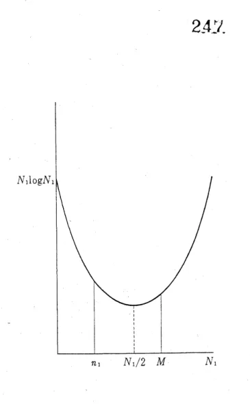
$H_{i}=H_{\max}$ $:=(1/N) \sum_{j}N_{i}\log N_{i}+\log N$ (atievalue)

245

thereexists $i$such that $\sigma_{Bi}^{2}\neq 0$ or _{$H_{i}\neq H_{\max}no$}

nev-selection occurs. Hence we have:

Theorem 4.10. Only the criterion $\Gamma_{A}$ is nev-free,

while the other criterza $\Gamma_{H}$ and $\Gamma_{D}$ may select a

nonessential variable.

The next example indicates that $\Gamma_{H}$ and $\Gamma_{D}$ do not

give even unique values to totally essential variables.

Example 4.13.

4.3.

Selection

of

a

totally

essential

vari-able (tev-bound property)

Any$tev$ is an optimal variable. Soit is desirablefor a

criterion to select a$tev$ whenever it exists. We show

that this is true for $\Gamma_{A}$ but not true for $\Gamma_{D}$ and $\Gamma_{H}$

.

As we will see below, not only alltevs donot give

ex-tremum values but non-tevs also can give extremum

values with respect to the both criteria $\Gamma_{D}$ and $\Gamma_{H}$

.

Thusin a sense, they are notsensitive to total

essen-tialityofa variable.

We have the following values of the criteria for each

variable.

Theorem 4.11. The criterion $\Gamma_{A}$ is tev-bound, while

$\Gamma_{H}$ and$\Gamma_{D}$ are not.

Proof.

Thisis derived from Lemma 3.1 and the

exam-plegiven below. $\square$

In thefollowing example all the variables (either

to-tally essentialornot)give tievalueswith respect to the

both criteria$\Gamma_{D}$ and $\Gamma_{H}$

.

Thus, we are not sure that

we do select an optimal variableas faras weobey the

criteria $\Gamma_{D}$ or $\Gamma_{H}$

.

Indeed, they may select anon-tev

1 which is not optimal. On the contrary the criterion

$\Gamma_{A}$ does not have this disadvantage.

Example 4.12.

In fact we have $H_{2}>H_{3}>H_{4}$ and $\sigma_{B_{2}}^{2}<\sigma_{B_{3}}^{2}<\sigma_{B_{4}}^{2}$

and the variable 3 is not $tev$ while the variables 2 and

4 are tevs. The criteria $\Gamma_{D}$ and $\Gamma_{H}$ select variable 4

(oneof the optimal variables), while $\Gamma_{A}$may select any

oftevs 1, 2 and 4.

4.4.

Selection of

a quasi-decisive

vari-able

(qdv-bound

property)

Lastly we will show that the

criteria

$\Gamma_{D}$ and $\Gamma_{H}$

are

qdv-bound while $\Gamma_{A}$ isnot, i.e. $\Gamma_{A}$ may select a

non-qdv even if there are $qdvs$

among

the variables of$f$

.

To show the qdv-bound property we mu$st$ show that

$qdvs$ give anextremum (maximumorminimum) value

ofthe criterion and, conversely,if there are $qdvs$, only

they (any of them) give an extremum value.

First we need anotation for treating a table having

qdvs which is used throughout this section. Assume

that $i$ is aO-side-qdv $(fi^{0}=a_{1})$, then _$f$ can be

repre-sented asfollows:

We have the following values of the criteria for each

246

So the condition thatthe variable$i$ isa O-side-qdv is:

$N_{1}^{i^{O}}$ $=$ $M$, $N_{j}^{1^{O}}$ _$=$ $0$for $j=2,$ $\ldots,$$K$, $N_{1}^{\dot{\iota}^{1}}$ $=$ $N_{1}-M$, $N_{j}^{:^{1}}$ _$=$ $N_{j}$ for $j=2,$ $\ldots,$$K$, where $M:=N/2=2^{L-1}(K\geq 2)$

.

Let $k$ be anyvariable of_{$f(k\neq i)$}

.

Put

$m_{j}$ $:=N_{j}^{k^{O}},$ $n_{j}$ $:=N_{j}^{k^{1}}$

$(m_{j}+n_{j}=N_{j}, \sum_{j}m_{j}=\sum_{j}n_{j}=M)$, (9)

$j=1,$$\ldots,$$K$.

Now we have a lemma.

Lemma 4.14. The vanable $k$ is also a $qdv$ in $f$

if

and only

_if

we have either $m_{j}=0(2\leq j\leq K)$ or

$n_{j}=0(2\leq j\leq K)$

.

Proof.

The necessity is easilyseen from the condition

that $k$ is also a $qdv$

.

Since then we can represent the

same table in the following form assuming that $k$ is

also decisivein O-side:

$qdvs$

.

This is easy to check for $\Gamma_{A}$ and $\Gamma_{H)}$ since

ac-tivities

are

$A;= \sum_{j=2}^{K}N_{j}=A_{k}$, and the entropy $H_{:}$

isdetermined by the

occurrence

frequencies ofactions

in the two subtables $fi^{S}$ (independently from its rule

configurations). For discriminant criterion, this is not

obvious. However, we have $N_{1}^{i^{1}}=N_{1}^{k^{1}}=N_{1}-M$,

$N_{j}^{:^{1}}=N_{j}^{k^{1}}=N_{j}(2\leq j\leq K)$ when both $i$ and $k$ are

O-side-decisive or $N_{1}^{k^{1}}=M,$ $N_{j}^{k^{1}}=0(2\leq j\leq K)$

when $k$ is l-side-decisive. In both cases, $\sigma_{Bi}^{2}=\sigma_{B_{k}}^{2}=$

$(1/4)(N/N_{1}-1)$

.

Actually, we prove amore stronger

result for each criterion in the sequel (i.e. every $qdv$

gives an extremum value with respect to each

crite-rion). We also prove that for activity criterion only a

maximum valueis not strictly attained by qdvs. This

property makes the activity criterion not qdv-bound.

Lemma 4.15.

_If

$i$ is a _$qdv$, then $A_{i}$ is a maximum.

Converse is not $trwe$

for

_$L>3,$ $i.e$. a maximum$A_{i}$ is

given not strictly by qdvs assuming there are qdvs, $in$

other words, $i$ may not be a _$qdv$ assuming that $A$_; is a

maximum and there are qdvs in $f$.

Proof.

Assuming $fi^{0}=a_{1},$$fi^{1}\neq$ const., we show $A_{k}\leq A_{i}$ for any $k$

.

Let $D$ denote the set of rules

having different actions from $a_{1}$ in $f^{i^{1}}$ (the

comple-ment $\overline{D}=fi^{1}\backslash D$ consists of rules having action

$a_{1})$

.

Then the activity $A;=|D|= \sum_{j=2}^{K}N_{j}$

.

Put $s:=|D|$ for simplicity. Foractive k-pairswe are

suffi-cientto consider only $fi^{1}$, sinceno active k-pai’r exists

in $fi^{0}$

.

Assume that there are $t$ active k-pairs within

$D$

.

Then the other possibility of active k-pair is

be-tween $D$ and $\overline{D}$

and the number of such k-pairs is at

most$s-2t$

.

Hence total number ofactivek-pairs are at most$A_{k}\leq s-2t+t=s-t\leq A_{i}$. The equality holds if

and only if$t=0$, which is satisfied if (but not only if)

theconditioninLemma 4.14 holds,i.e. $k$ isalsoa$qdv$

.

Forthe second assertionwe give an example below. $\square$

Inthe followingexample weshow that$A_{k}=A_{i}=s$

(a maximumamong all variables) for a$qdvi$ and for a

non-qdv $k$

.

Thus$\Gamma_{A}$ isnot qdv-bound in this case.

Then obviously $m_{j}=0$ for $j=2,$$\ldots k$

) The latter

alternativeoccurs when$k$isl-side-quasi-decisive. This

is obtained byexchangingvectors of$x_{k}=0$and$x_{k}=1$

in $fi^{1}$ so that the action $a_{1}$ covers$x_{k}=1$

.

Conversely,

assume that $m_{j}=0$for$j=2,$$\ldots$,$K$. Then from (??)

we have $n_{j}$ $:=N_{j}^{k^{1}}=N_{j}$ for $j=2,$$\ldots$,$K,$ $N_{1}^{k^{O}}=M$

and $N_{1}^{k^{1}}=N_{1}-M$

.

_{This means that} $k$ is also a

0-side-qdv. $\square$

We note that all the three

criteria

$\Gamma_{A},$ $\Gamma_{H}$ and

$Gamma_{D}$ give the same values, respectively, for all

Example 4.16. We represent a 4-ary function

$f(x_{1}x_{2}x_{3}x_{4})$ by giving$f1^{0}$ and $f1^{1}$:

$f1^{0}$ _$:=a$, _{$f1^{1}(000)=b$}, _{$f1^{1}(011)=c$},

$f1^{1}(110)=d$, $f1^{1}(x_{2}x_{3}x_{4})=a$ for other $x_{2}x_{3}x_{4}$

.

Wehave $A;=3$ for all $i=1,2,3,4$ ($t=0$ in all cases)

but only the variable 1 is $qdv$.

Wenote that only for 2-ary tables $(L=2)$ the

con-verse of the lemma holds, i.e. the conditions $A_{1}=$

$A_{2}=a$

maximum

andvariable 1 is $qdv$ imply

variable

$2_{-}4_{-}^{\triangleright}J$

.

Lemma 4.17.

_If

$i$ is a _$qdv$ then $H_{i}$ is a minimum.

Conversely,

_if

there are qdvs, then only qdvs give a

minimum value

_of

$H_{1}$

.

Proof.

Let $fi^{0}=a_{1}$ and $k$ be any variable _{$(k\neq i)$}

.

We show$H;\leq H_{k}$ and the equality holds (if and) only

if $k$ is also a $qdv$. Denote the number of rules having

action$a_{1}$ and $x_{k}=0$ in$fi^{1}$ by$m_{1}’$ and similarly by$n_{1}’$

for $x_{k}=1$. That is $m1$ $;=$

$|$

{

$(x,$$f(x))$ havingaction

$a_{1}$ and $x_{i}=1,$ $x_{k}=0$

}

$|$,

$n_{1}’$ _$;=$

$|$

{

$(x,$$f(x))$ havingaction

$a_{1}$ and $x;=1,$ $x_{k}=1$

}

$|$

.

Since rules of $fi^{0}$ consist exactly the same number

$(M/2)$ ofvectors of$x_{k}=0$ and $x_{k}=1$, we have (cf.

(9))

$m_{1}=M/2+m_{1}’,$ $n_{1}=M/2+n_{1}’(N_{1}-M=m_{1}’+n_{1}’)$

.

(10) From$p_{j}^{i}=N_{j}^{i}/M$we have for $i$ and $k$:

$p^{i_{1^{O}}}=1,$ $p_{j^{o}}^{i}=0$ for $j=2,$

$\ldots$,$K$, $p_{1}^{i^{1}}=(N_{1}-M)/M,$ $p_{j^{1}}^{i}=N_{j}/M$ for $j=2,$

$\ldots$,$K$,

$p_{j}^{k^{0}}=m_{j}/M$ for _$j=1,$

$\ldots$,$K$,

$p_{j}^{k^{1}}=n_{j}/M$ for _$j=1,$

$\ldots,$$K$.

Substituting these into (3), we have (hereafter all the

summation is for $2\leq j\leq K$ unless explicitly stated in

other way):

$s$ $:=-N(H;-H_{k})=(N_{1}-M)\log(N_{1}-M)/M$

$+ \sum(N_{j}\log N_{j}/M)-\sum_{j=1}^{K}(m_{j}\log m_{j}/M$

$+n_{j}\log n_{j}/M)$

$=(N_{1}-M)\log(N_{1}-M)-(m_{1}\log m_{1}+n_{1}\log n_{1})$ $+M \log M+\sum(N_{j}\log N_{j}-m_{j}\log m_{j}-n_{j}\log n_{j})$.

Again, substituting $m_{j}=N_{j}-n_{j},$ $j=1,$$\ldots,$$K$, we

have $s=(N_{1}-M)\log(N_{1}-M)$ $+M\log M-(N_{1}-n_{1})\log(N_{1}-n_{1})-n_{1}\log n_{1}$ $+ \sum((N_{j}-n_{j})\log N_{j}/(N_{j}-n_{j})+n_{j}\log N_{j}/n_{j})$

.

Putting$t(x)=(N_{1}-x)\log(N_{1}-x)+x1ogx$, $s=t(M)-t(n_{1})$ $+ \sum((N_{j}-n_{j})\log N_{i}/(N_{j}-n_{j})+n_{j}\log N_{j}/n_{j})$

.

Figure 4: The function $t(x)=(N_{1}-x)\log(N_{1}-x)+$

$x\log x(0\leq x\leq N_{1})$

.

From $N_{j}\geq n$; the last term is non-negative $(\geq 0)$

.

We show that $k$isa_$qdv$ ifand only if_{$t(M)\leq t(n_{1})$}.

The function$t(x),$ $0\leq x\leq N_{1}$ is a monotone

symmet-ricwith respect to $x=N_{1}/2$ (cf. Fig. 4). Considering

$n_{1}\leq M,$ $N_{1}/2\leq M\leq N_{1}$, wehave

$n_{1}\leq N_{1}/2-(M-N_{1}/2)=N_{1}-M\Leftrightarrow t(M)\leq t(n_{1})$

.

(11)

Substituting (10) into (11), we conclude $t(M)$ $\leq$

$t(n_{1})\Leftrightarrow M/2\leq m_{1}’$

.

Since there are another $M/2$

ruleshaving action $a_{1}$ an$dx_{k}=0$ (amongthe rulesof

$x_{i}=0)$, this means that $k$ is also O-side-decisive, i.e.

$fk^{0}=a_{1}$ (a constant). Hence, if$k$ is not a $qdv$, then

$s>0$

.

Thus, whenever a$qdv$ exists, a $qdv$ is selected

(ifthere are many qdvs thenany of them, becausethey

giveatievalue),since weselect a variable$i$whichgives

aminimal value of$H_{i}$

.

$\square$

Lemma 4.18.

_If

$i$ is a _$qdv$, then $i$ gives a maximum

value

_of

$\sigma_{Bi}^{2}$. Conversely,

if

there are qdvs then only

qdvs give a maximum value

_of

$\sigma_{Bi}^{2}$

.

248

$(1/N) \sum_{j}(N_{j}^{i^{1}})^{2}/N_{j}$

.

Putting $N_{j}’$ $:=N_{1}\cdots N_{j-1}$

.

$N_{i+1}\cdots N_{K}$,we have$N \cdot N_{1}\cdots N_{K}\cdot B;=\sum_{j}N_{j}’(N_{j}^{i^{1}})^{2}$

.

Following thenotation (10)for the variable$k$, consider

$h$

$:=N \cdot N_{1}\cdots N_{K}(B_{i}-B_{k})=\sum_{j=1}N_{j}’((N_{j}^{i^{1}})^{2}-n_{j}^{2})$

.

Substituting $N\dot{i}^{1}=N_{1}-N/2$ and $n_{1}=N/2- \sum^{(13)}n_{j}$

into (13), we have thefollowing:

$h=N_{1}’(N_{1}-N/2)^{2}+ \sum N_{j}’N_{j}^{2}$ $-N_{1}’(N/2- \sum n_{j})^{2}-\sum N_{j}’n_{j}^{2}$

$=N_{1} \cdots N_{K}(\sum_{j=1}N_{j}-N)+N_{1}’(N^{2}/4)$

$-(N_{1}’(N^{2}/4-N \sum n_{j}+(\sum n_{j})^{2})-\sum N_{j}’n_{j}^{2}$ $=N_{1}’N \sum n_{j}-N_{1}’(\sum n_{j})^{2}-\sum N_{j}’n_{j}^{2}$

.

Again, substituting $N= \sum_{j=1}^{K}N_{j}=N_{1}+\sum N_{j}$ into

this, we have

$h=N_{1}’N_{1} \sum n_{j}$

$+N_{1}’( \sum n_{j})\sum N_{j}-N_{1}’(\sum n_{j})^{2}-\sum N_{j}’n_{j}^{2}$

.

Using

_N\’i

$N_{1} \sum n_{j}=\sum N_{j}’N_{j}n_{j}$, wefinally have

$h= \sum N_{j}’N_{j}n_{j}$

$- \sum N_{j}’n_{j}^{2}+N_{1}’(\sum n_{j})(\sum(N_{j}-n_{j}))$

$= \sum N_{j}’n_{j}(N_{j}-n_{j})+N_{1}’(\sum n_{j})(\sum(N_{j}-n_{j}))$

$\geq 0$.

The equality holds strictly either $n_{j}=0$ for $j=$

$2,$

$\ldots,$$K$or $N_{j}=n_{j}$ for$j=2,$$\ldots,$$K$

.

Thismeans that

the equality$\sigma_{Bi}^{2}=\sigma_{Bk}^{2}$ holds whenand onlywhen the

variable $k$is alsoa $qdv$fromLemma4.14. $\square$

From Lemmas 4.15,4.17,4.18, we have the following

theorem.

Theorem 4.19. The two cmteria$\Gamma_{H}$ and$\Gamma_{D}$ are

qdv-bound, while $\Gamma_{A}$ is not.

5.

Discussions

and

Conclusions

An efficient VSM (variable selection method

accord-ing to a criterion) constructs a near optimum tree in

theaveragemuch less computation than the worstcase

evaluation $O(L^{2}2^{L})$ with $O(L2^{L})$ storage, where $L$ is

the number ofvariables of the table.

Inthis paperwe have developed the threecriteria for

such VSM from three different standpoints: $\Gamma_{A}$

(activ-ity criterion) from combinatorial,$\Gamma_{H}$from entropy and

$\Gamma_{D}$fromdiscriminant analyses, for constructingan

op-timum tree in the sense of the number of nodes ofthe

tree.

The three criteriahave been examined with respect

to the conditions which an optimum criterion should

satisfy: rejection of nonessential variables (nev-free),

selection of a totally essential variable and a

quasi-decisive variable (tev-bound and qdv-bound properties;

both $tev$ and $qdv$ are optimal variables). We have

shown that $\Gamma_{A}$ is nev-free, tev-bound but not

qdv-bound, while the two criteria $\Gamma_{H}$ and $\Gamma_{D}$ are neither

nev-free nor tev-bound but qdv-bound. It is hard to

claim thatonecriterionis better thanothersonlyfrom

these considerations. Consequently, a series of

exper-iments‘was done, comparing the costs of these near

optimum trees also with those of optimum trees. It

shows that activitycriterionis slightly better than

oth-ers(1.03 versus 1.05in terms of optimality coefficient)

with comparable computation; the other two indicates practically identical performance.

Entropy of a variable is defined simply through

oc-currencefrequencies ofall actionsregardless its

struc-ture in the conditional part an$d$ discriminant criterion

inspects the rules in which the bit ((1) is _standing in

thecorresponding variable, while activity of a variable

takesintoaccount also the values of the other variables

in the rule to some extent. This difference may have

producedtheslightly better coefficient for the activity.

An extension ofthe criteria to the casethat testing

a variable$i$ incurs a certain cost $C_{i}$ depending on the

variable (general “description cost”) may be to use a

quantity given by dividing the value of the described

criterion by $C_{1}$ as a new criterion. Then, however, for

such criteriaone can not prove any of the formal

prop-erties whichwe have showninthis paper, although the

properties that$nev$ is a worst and$tev$ and $qdv$ are

op-timal variablesremain valid.

VSM criteriafor the case when the cost ofa tree is

definedastheaveragecost oftesting canbeobtainedin

thesameway. We have observed a similar experimental

result concerning the comparative performance of the

threecriteria. The combinatorialcriterionfor this cost

has also been studiedin more detail in [Miy89].

The newly introduced discriminant criterion $\Gamma_{D}$ has

an evident computational advantage over entropic

cri-terion $\Gamma_{H}$, although the required numbers of basic

op-erations (bit-test) remain the same order. This

direc-tion would provide us further development of the

249

Acknowledgement

Thefirst author wishesto dedicate this paper to the

memory of the late Hitoshi Miyakawa.

References

[Bay73] Bayes A.J.: A dynamic programming

algo-rithm to optimise decision table code.

Aus-tralian Computer J. 5, 2 (May 1973), 77-79.

[Bud85] Budach L.: A lower bound for the number of

nodes in a decision trees, Electron Inf. verarb.

Kybern. EIK 21 (1985) 4/5, 221-228.

[Cha87] Chan, A. H.:Using decision trees to derive

the complement of a binary function with

multiple-valued inputs, IEEE Trans. on

Com-put., C-36, 2, 1987, 212-214.

[Fis36] FisherR.A. The use of multiple measurements

in taxonomicproblems, Ann.Eugenics,7, Part

II, 179-188 (1936).

[Gar72] Garey, M.R.: Simple Binary identification

problems. IEEE Tkans. Comput. TC-21, 6,

588-590, June 1972.

[Gan73] Ganapathy.S., Rajaraman, V.: Information

theoryappliedto theconversion of decision

ta-bles to computerprograms. Comm. ACM, 16,

9, 532-539, Sept., 1973.

[HVMG82] Hartman, C.R.P.,Varshney, P.K.,

Mehro-tra,. K.G., Gerberich, C.L.: Application of

in-formation theory to the construction of

effi-cient decision trees. IEEE ’hans. on

Informa-tion theory IT-28,4, 565-577, July 1982.

[HyR76] Hyafil,L.,Rivest,R.L.: Constructingoptimal

binary decision trees is NP-complete. Comm.

ACM 5, 1, 15-17, May 1976.

[Knu73] Knuth, D.E.: The art ofcomputer

program-ming,vol. 1,2nded.Reading,Mass.:

Addison-Wesley, 1973.

[Knu73] Knuth, D.E.: The art ofcomputer

program-ming,vol. 3,Reading, Mass.: Addison-Wesley,

1973.

[Lov85] Loveland, D. W,: Bounds for binary testing

with arbitrary weights, Acta Informatica 22,

101-114, 1985.

[MiS80] Miyakawa, M., Sabelfeld, V.K.: On

mini-mizations of size of logical schemes (in

Rus-sian).Theoretical basisofcompiling (A. P.

Er-shov, ed.), 49-58, Novosibirsk State University,

Novosibirsk 1980.

[MiO82] Miyakawa, M., Otsu, N.: Algorithms for

constructing near-minimum total nodes

de-cision trees from expanded decision tables

(Japanese). TGEC IECE Japan, EC82-33,

July 1982.

[Miy85] Miyakawa, M.: Optimum decision trees - an

optimalvariabletheoremanditsrelated

appli-cations-. Acta Informatica 22, 475-498, 1985.

[Miy89] Miyakawa, M.: Criteriafor selectingavariable

in the construction of efficient decision trees,

IEEE Trans. Comput., to appear.

[MTG80] Moret, B.M.E., Thomason, M.G., Gonzalez,

R.C.: The activity of a variable and its

rela-tionto decision table. ACM Trans. Prog. Lang.

Syst. 2,4, 580-595, Oct. 1980.

[MTG81] Moret, B.M.E., Thomason, M.G., Gonzalez,

R.C.: optimization criteriafor decision trees,

Dept. of Computter Science, Collage of

Engi-neering, University of New Mexico, Technical

Report CS81-6, 1981.

[Mor82] Moret, B.M.E.: Decision trees and diagrams.

ComputingSurveys 14, 4, 593-623, Dec. 1982.

[Res66] Reinwald, L.T., Soland, R.M.:

Conversion

of

limited-entry decision tables to optimal

com-puterprogramsI:minimum average processing

time. JACM 13, 3, 339-358, July 1966.

[ReS67] Reinwald, L.T., Soland, R.M.: Conversion of

limited-entry decision tables to optimal

com-puter programs II: minimum storage

require-ment. JACM 14, 4, 742-755, Oct. 1967.

[Sas85] Sasao, T: An algorithm to derive the

com-plement of a binary function with

multiple-valued inputs, IEEETrans.on Comput.,C-34,

2, February 1985, 131-140.

[ScS76] Schumacher, H., Sevcik, K.:The synthetic

ap-proach to decision table conversion. Comm.

ACM 19, 6, 343-351, June 1976.

[Spr66] Sprague V. G.: On storage space of decision

trees. Comm. ACM 9, 5, 319-319, May 1966.

[Ver72] Verhelst M.: The conversion oflimited-entry

decision tables to optimal and near optimal

flowcharts: two new algorithms. Comm.ACM

15, 11, 974-980, November 1972.

[Weg84] Wegner I.: Optimal decision trees and

one-time-only branching programs for symmetric

Boolean functions. Information and Control