JAIST Repository: Research on the Common Developments of Plural Cuboids

全文

(1)Research on the Common Developments of Plural Cuboids. By Xu Dawei. A thesis submitted to School of Information Science, Japan Advanced Institute of Science and Technology, in partial fulfillment of the requirements for the degree of Master of Information Science Graduate Program in Information Science. Written under the direction of Professor Ryuuhei Uehara. September, 2014.

(2) Research on the Common Developments of Plural Cuboids. By Xu Dawei (1210214). A thesis submitted to School of Information Science, Japan Advanced Institute of Science and Technology, in partial fulfillment of the requirements for the degree of Master of Information Science Graduate Program in Information Science. Written under the direction of Professor Ryuuhei Uehara and approved by Professor Ryuuhei Uehara Professor Hajime Ishihara Professor Kunihiko Hiraishi. August, 2014 (Submitted). c 2014 by Xu Dawei Copyright .

(3) Contents 1 Introduction 1.1 Research background and aim . . . . . . . . . . . . . . . . . . . . . . . . . 1.2 Content of thesis . . . . . . . . . . . . . . . . . . . . . . . . . . . . . . . .. 1 1 1. 2 Preliminaries 2.1 Development and cuboid . . . . . . . . . . . . . . . 2.2 Theorem about development . . . . . . . . . . . . . 2.3 Incongruent orthogonal boxes with the same surface 2.4 Existing algorithm . . . . . . . . . . . . . . . . . . 2.5 Partial common development . . . . . . . . . . . .. 3 3 3 4 5 5. . . . . . . area . . . . . .. . . . . .. . . . . .. . . . . .. . . . . .. . . . . .. . . . . .. . . . . .. . . . . .. . . . . .. . . . . .. 3 Enumeration Algorithm 3.1 Enumeration algorithm of common developments of three incongruent orthogonal boxes . . . . . . . . . . . . . . . . . . . . . . . . . . . . . . . . . 3.2 Data structure . . . . . . . . . . . . . . . . . . . . . . . . . . . . . . . . . . 3.3 Box checking of developments . . . . . . . . . . . . . . . . . . . . . . . . . 3.3.1 Checking algorithm . . . . . . . . . . . . . . . . . . . . . . . . . . . 3.3.2 Direction deviation . . . . . . . . . . . . . . . . . . . . . . . . . . . 3.4 Generate of developments . . . . . . . . . . . . . . . . . . . . . . . . . . . 3.4.1 New square has three adjacency blank . . . . . . . . . . . . . . . . 3.4.2 New square has two adjacency blanks (up and down, left and right) 3.4.3 New square has two adjacency blanks (up and left, up and right, down and left, down and right) . . . . . . . . . . . . . . . . . . . . 3.4.4 New square has one adjacency blank . . . . . . . . . . . . . . . . . 3.4.5 New square has no adjacency blank . . . . . . . . . . . . . . . . . . 3.5 Normalization of developments . . . . . . . . . . . . . . . . . . . . . . . . . 3.6 Comparison between developments . . . . . . . . . . . . . . . . . . . . . . 3.6.1 Compression . . . . . . . . . . . . . . . . . . . . . . . . . . . . . . . 3.6.2 Storage . . . . . . . . . . . . . . . . . . . . . . . . . . . . . . . . .. 6 6 8 9 9 12 14 15 15 15 15 17 17 18 18 18. 4 Common Developments of incongruent orthogonal boxes 20 4.1 Common developments of boxes of sizes 1×1×7 and 1×3×3 of surface area 30 . . . . . . . . . . . . . . . . . . . . . . . . . . . . . . . . . . . . . . . . 20 4.1.1 Experiment environment . . . . . . . . . . . . . . . . . . . . . . . . 20 i.

(4) 4.2. 4.1.2 Result . . . . . . . . . . . . . . Common developments of boxes of sizes of surface area 30 . . . . . . . . . . . . 4.2.1 Experiment environment . . . . 4.2.2 Result . . . . . . . . . . . . . .. 5 Conclusion. . . . . . . . . . 1×1×7, 1×3×3 . . . . . . . . . . . . . . . . . . . . . . . . . . .. . . . √. . .√. . √ . . and 5× 5× 5 . . . . . . . . . . . . . . . . . . . . . . . . . . . . . .. . 20 . 24 . 24 . 24 27. ii.

(5) Chapter 1 Introduction 1.1. Research background and aim. In 1525, the German painter and thinker Albrecht D¨ urer published his masterwork on geometry “On Teaching Measurement with a Compass and Straightedge”, which opened an area with a lot of open problems[1]. Lubiw and O’Rourke started investigating polygons that can fold into polyhedra in 1996[2]. In 2007, Demaine and O’Rourke published a scholarly book, which is about geometric folding algorithms[3]. In this paper, we study common developments that can fold into two or more incongruent orthogonal convex polyhedra, that is boxes. Those common developments are obtained by cutting along their unit lines. These developments are simple polygons that consist of unit squares of four connected so that the boxes and their corresponding developments have the same surface area. In searching for common developments that fold into two or more incongruent orthogonal boxes, we start from a relative simple task: finding two or more incongruent orthogonal boxes whose surface areas are equal but sizes are different. The smallest surface area that different orthogonal boxes can appear is 22 which admits to fold into two boxes of size 1×1×5 and 1×2×3. All common developments of these two boxes have been already known[4][5]. The next smallest integer N such that surface area N can fold into two different boxes is 30. Matsui tried to list the common developments of two different boxes of sizes 1×1×7 and 1×3×3 of surface area 30, but failed due to the limitation of computational power[5]. We filled this gap and research further. √ We√had√already known another polygon that can fold into boxes of size 1×1×7 and 5× 5× 5, whose surface area is also 30. So next we try to find a polygon of surface area 30 that folds into above three different boxes. It is a great improvement from previous known one that the smallest surface area that folds into three different boxes is greater than 500[6]. To achieve that we propose a new efficient algorithm.. 1.2. Content of thesis. The second chapter is preliminaries of thesis, we gave a definition to the common developments we explorer in the research, and a description of existing algorithm. 1.

(6) The third chapter shows the detail of the algorithm of finding common developments of incongruent orthogonal boxes, and some explanations of key points. The fourth chapter shows the result of the research. The fifth chapter is the conclusion and future works.. 2.

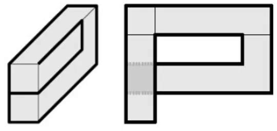
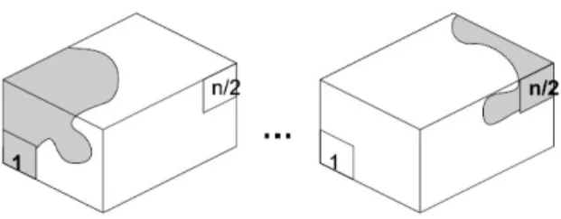
(7) Chapter 2 Preliminaries 2.1. Development and cuboid. The development is simple polygon that consist of unit squares of four connected. In this way, the orthogonal box and its corresponding developments have the same surface area n. When unfolding a cuboid along the edge, there can be a overlap on the final development as Fig. 2.1. Also, if there is a hole inside the development, all eight directions of its adjacency squares should be occupied by unit squares of the development. Or that hole may be a vertex of the cuboid in fact. In other words, a hole on the development should have no adjacency blanks (Fig. 2.2). A development with a hole or an overlap is not what we want to talk about in this paper, for they cannot fold into a box with the same surface area.. Figure 2.1: Development with a overlap. 2.2. Theorem about development. The following is the existing theorem about the development.. 3.

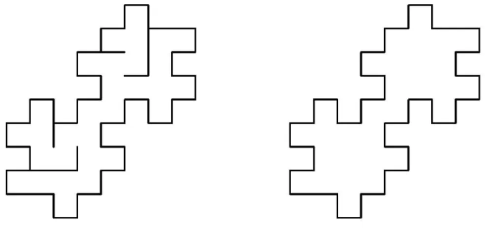
(8) Figure 2.2: Development with a hole (left), development without a hole (right). Theorem[7]: Let P be a polygon that can fold to a box B. If P has a cut inside, we glue it and obtain P’ with no cut inside. Then P’ also can fold to B (Fig. 2.3).. Figure 2.3: Development with a cut (left), development with no cut (right). Proof: Since B is a convex orthogonal box, it follows. If we fold a polygon into a box start around the cut, the cut should not contain any square from other side of the polygon, or the interior angles sum is larger than 360 degrees, which creates a non convex polyhedron, not a box. Therefore, according to this theorem, we only consider developments with no cut inside.Also, even if a development has a cut inside, which cannot fold into another box using the cut.. 2.3. Incongruent orthogonal boxes with the same surface area. In searching for common developments that fold into two or more incongruent orthogonal boxes whose surface areas are equal but sizes are different. We have such a set: P (S )={(a, b, c)|(ab+bc+ac)×2=S }(S, a, b, c are positive integers,0<a≤b≤c). When |P (S )|≥2, the cuboid with size (a, b, c) can have a development. The list of incongruent orthogonal 4.

(9) boxes with the same surface area is shown below.. .. .. • • • • • • • • • • •. P (22)={(1, 1, 5), (1, 2, 3)} P (30)={(1, 1, 7), (1, 3, 3)} P (34)={(1, 1, 8), (1, 2, 5)} P (38)={(1, 1, 9), (1, 3, 4)} P (46)={(1, 1, 11), (1, 2, 7), (1, 3, 5)} P (54)={(1, 1, 13), (1, 3, 6), (3, 3, 3)} P (58)={(1, 1, 14), (1, 2, 9), (1, 4, 5)} P (62)={(1, 1, 15), (1, 3, 7), (2, 3, 5)} P (64)={(1, 2, 10), (2, 2, 7), (2, 4, 4)} P (70)={(1, 1, 17), (1, 2, 11), (1, 3, 8), (1, 5, 5)} P (88)={(1, 2, 14), (1, 4, 8), (2, 2, 10), (2, 4, 6)}. • The smallest surface area that different orthogonal boxes can appear is 22 which admits to fold into two boxes of size 1×1×5 and 1×2×3. All common developments of these two boxes have been already known. The next smallest integer N such that surface area N can fold into two different boxes is 30.. 2.4. Existing algorithm. In searching for common developments of two different boxes of sizes 1×1×7 and 1×3×3 of surface area 30, we applied the algorithm that connects a unit square at a time at random from scratch. It first starts from one unit square. By connecting unit squares at each edge, many partial common developments are generated. Finally unit squares are increased to the size of the surface area of given orthogonal boxes.. 2.5. Partial common development. Common developments obtained by unfolding part of the cuboids, we call it partial common developments. It can be a part of the final common development, and can fold into many different part of target boxes. With unit squares increasing, the partial common development can finally become the normal common development.. 5.

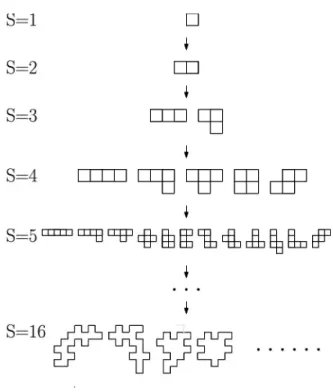
(10) Chapter 3 Enumeration Algorithm 3.1. Enumeration algorithm of common developments of three incongruent orthogonal boxes. The algorithm operates in the following steps. Input : The edge length (a1 , b1 , c1 ), (a2 , b2 , c2 ), (a3 , b3 , c3 ) of three incongruent orthogonal boxes B1 , B2 and B3 . Output: The common developments of incongruent orthogonal boxes B1 , B2 and B3 . Step 1 Start from a partial development of surface area 1. Step 2 Maintain a relationship diagram of boxes B1 , B2 and B3 , for it can be checked in next steps. Step 3 Check the partial developments generated. Test whether each partial development can fit on boxes B1 , B2 or not (B1 , B2 are boxes of sizes 1×1×7 and 1×3×3, we study these common developments first for it is the remaining issues of previous research), any partial development that cannot fit all the box should be omitted. If there is a partial common development passed all box check, add one square to one of its adjacency blank, making is surface area one plus. If the new partial common development has the same shape with the old partial common developments that already generated, then it will be omitted. The same shape means the rotation and mirror images of the original development. Step 4 To increase the partial common developments to normal common developments, repeat the step 2 and step 3. When adding new one square to the partial development, we need to check whether there is a hole inside the partial development(Fig. 3.1). Step 5 When the surface area of partial common developments is increased to 16, 6.

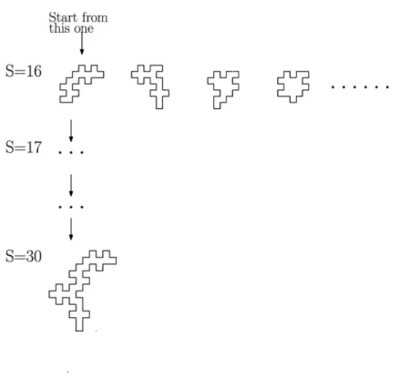
(11) Figure 3.1: Change of partial developments with the increasing of surface area. divide the partial developments generated this step into small groups (102400 partial developments per group). Step 6 Process these small groups on super computer one after one, continue process from step 17 to final step of 30 (Fig. 3.2). Step 7 Merge the result of each small group, the outcome is the common developments of boxes B1 , B2 . Thus, the searching of common developments of two incongruent orthogonal boxes finishes. Step 8 Based on the result of previous step, check whether each common development can fit on the box B3 . Those developments pass the check at the final step of surface area 30 are common developments that can fold into incongruent boxes B1 , B2 and B3 . During the processing, the image of partial developments with surface area increasing shows like a wave, it has a summit at some point. As shown in the result. 7.

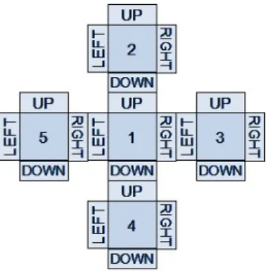
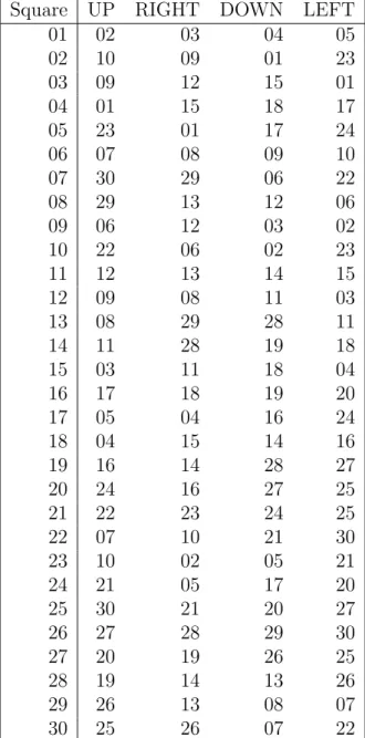
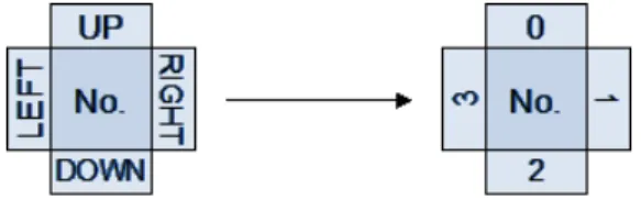
(12) Figure 3.2: Process these small groups one after one. 3.2. Data structure. Since we are studying cuboids, its unit squares are each four side connected, and numbered. Therefore, in this research developments are represented by the matrix of 0 and 1 (Fig. 3.3).. Figure 3.3: Matrix and corresponding development We use a array to represent the position relationship of cuboid. Every cuboid has its unique position relationship of unit squares (Fig. 3.4, Table 3.1). Every unit square on the cuboid has four unique adjacency neighbors in four numbered directions. Thus we can tell a development can fold into the target cuboid or not. Every unit square is numbered from 1 to 30 and the rest of item are its neighbors in UP, RIGHT, DOWN, 8.

(13) LEFT directions (Fig. 3.5).. Figure 3.4: Position relationship graph of cube of size. √. √ √ 5× 5× 5. Figure 3.5: Structure of unit square. 3.3 3.3.1. Box checking of developments Checking algorithm. Previous study mainly focus only on the ”normal” orthogonal polyhedra, which are cuboids with an integer edge length. Program can simulate the box with few arrays to represent its structure. The gap between the element can be seen as the edge of unit squares and development also fold along the edge. It is relative easy to check whether the partial development can fit the boxes or not (Fig. 3.6). √ √ √ However, the development of the cube of 5× 5× 5 cannot fold along the edge of unit squares, which means the previous method of check the development can fit the box or not is no more available. We have two algorithms for the approach of checking the 9.

(14) Table 3.1: Position relationship table of cube of size Square UP RIGHT 01 02 03 02 10 09 03 09 12 04 01 15 05 23 01 06 07 08 07 30 29 08 29 13 09 06 12 10 22 06 11 12 13 12 09 08 13 08 29 14 11 28 15 03 11 16 17 18 17 05 04 18 04 15 19 16 14 20 24 16 21 22 23 22 07 10 23 10 02 24 21 05 25 30 21 26 27 28 27 20 19 28 19 14 29 26 13 30 25 26. 10. DOWN 04 01 15 18 17 09 06 12 03 02 14 11 28 19 18 19 16 14 28 27 24 21 05 17 20 29 26 13 08 07. √. LEFT 05 23 01 17 24 10 22 06 02 23 15 03 11 18 04 20 24 16 27 25 25 30 21 20 27 30 25 26 07 22. √ √ 5× 5× 5.

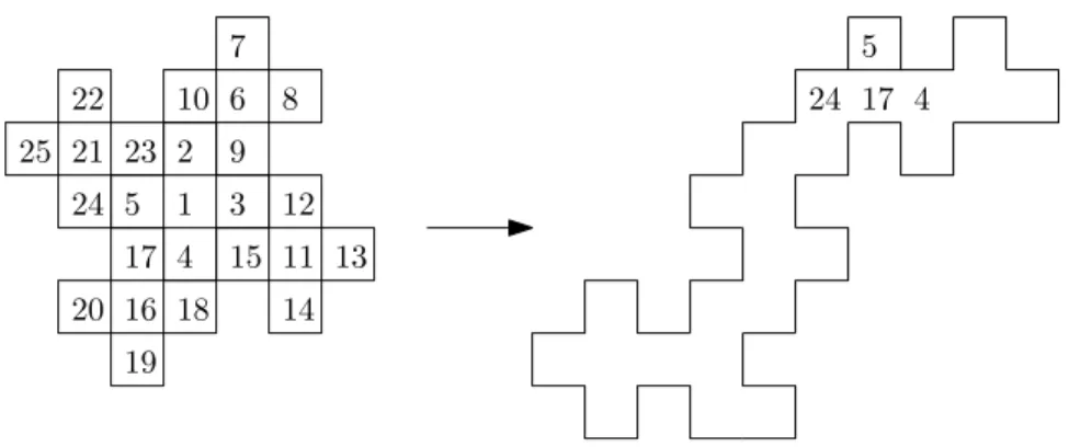
(15) Figure 3.6: Previous method cannot apply for cube of. √. √ √ 5× 5× 5. √ √ √ cube of 5× 5× 5, one algorithm is checking for each P the vertex of the cube on the development boundary. Since the surface of cube is also square, an angle of 26.6 degrees exist between its edge and the unit square’s edge. Besides, a vertex is made of three planes, which means every vertex on the development should be surrounded by 3 squares. Therefore, we need to check whether there is a development fit such requirements: all vertices of the cube are on the boundary of development, constituting a cross network with 26.6 degrees to the unit square’s edge, squares around all vertices should be exactly 24. The second algorithm is checking the positional relationships of each unit square on the development. Every polyhedron, including cube, as long as it has a development made of a certain kind of basic shape, the positional relationships of each unit shape does not change with different development. In this point, if in any development, √ √ √ its unit squares have the same positional relationships even on the cube of 5× 5× 5 we can identify if it can fold into that cube. The first algorithm can not consider the dislocation of center square, which actually makes a hole and an overlap on the cube. Therefore, the second algorithm is more feasible in this paper. The detail of algorithm shown as below. Step 1 After we obtained the position relationship table of the target cuboid, we mark one unit square on the partial development as ”start point” (Basically, the square at top left for it is always the first visited in traversal). √ √ √ Step 2 Since there are six surfaces on the cuboid of size 5× 5× 5, we use one surface to start matching. Besides, one surface of the cuboid has five squares, we mark them as s1 , s2 , s3 , s4 , s5 (Other 25 squares can be obtained by rotation and makes no difference). Step 3 Assume the partial development can fold into the part of the target cuboid as the start point is located as s1 (Start point can be any one of s1 , s2 , s3 , s4 , s5 ), then give start point the number that s1 marked and the UP neighbor of start point should be marked as the UP neighbor of s1 and given the number of the neighbor of s1 , so do the rest three directions (Fig. 3.7). If there is no neighbor of start point in some direction, then skip it. 11.

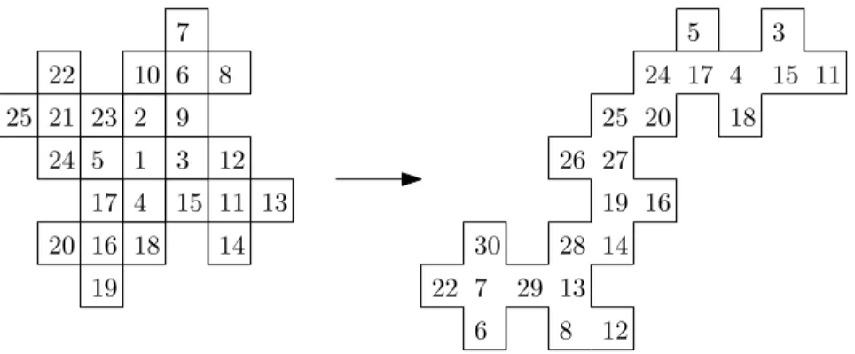
(16) 7 22. 10 6. 25 21 23 2. 9. 24 5. 3. 1. 17 4. 5 8. 17. 12. 15 11 13. 20 16 18. 14. 19. Figure 3.7: Example of start point marked as s5 , step 3. Step 4 Now we finished with start point, mark other unit squares given a number as a new start point and repeat step 3 (Fig. 3.8).. 7 22. 10 6. 25 21 23 2. 9. 24 5. 3. 1. 17 4 20 16 18. 5 8. 24 17 4. 12. 15 11 13 14. 19. Figure 3.8: Example of start point marked as s5 , step 4. Step 5 If all squares of the partial development are mark with different numbers, this partial number pass the check(Fig. 3.9). If any two squares are marked with the same number, that means an overlap on the development and this development cannot pass the check. Step 6 Repeat step 1 to 5, mark the start point as another square of s1 , s2 , s3 , s4 , s5 . It should be different than the previous one.. 3.3.2. Direction deviation. A normal direction relationship should be UP to DOWN, LEFT to RIGHT. But when there is an edge between two squares, things are different.. 12.

(17) 7 22. 10 6. 25 21 23 2. 9. 24 5. 3. 1. 17 4 20 16 18 19. 5 8. 3. 24 17 4 25 20. 12. 15 11. 18. 26 27. 15 11 13. 19 16. 14. 30 22 7 6. 28 14 29 13 8. 12. Figure 3.9: Example of start point marked as s5 , step 5. Figure 3.10: Position relationship across the edge. 13.

(18) As Fig. 3.10 shows, the UP of square 12 is 9 and the RIGHT of square 12 is 8, but the DOWN of square 9 is 3 and the LEFT of square 8 is 6. Because there is an edge between these squares, their direction relationship have a deviation.. Figure 3.11: Example of error occurs on a correct development In some parts of developments like Fig. 3.11, RIGHT of square 9 need to be marked. By checking the position relationship table, it should be 12. Besides, UP of 12 is also need to be marked. It is marked as 9 again. But in fact it should be 8, which causes an error.. Figure 3.12: Using numbers to represent directions. Every time a position relationship across an edge, the axis of the direction of the square rotate 90 degree to the original axis of position relationship table. To solve this problem, we use numbers to represent directions (Fig. 3.12), and propose a formula below: deviation=[(direction from previous)-(direction from current)+2+old deviation]%4 In this fomula, from square 9 to 12, the deviation=(1-0+2+0)%4=3, which is 270 degrees clockwise. Thus the UP of square 12 is in fact the RIGHT of square 12, which is square 8.. 3.4. Generate of developments. A new development is generated by adding a square to the adjacency blank of an existing partial development (Fig. 3.13). Repeat this step and we can obtain the final development. However, a hole inside the development can appear during this step. To generate a development with no hole inside it is necessary to consider what is around the new added square. 14.

(19) Figure 3.13: Possible results of adding one square. 3.4.1. New square has three adjacency blank. Newly added square has only one neighbor square. In this situation, a hole inside is impossible to appear (Fig. 3.14).. Possible ?. Blank. ?. Blank New. ?. Blank. ?. Figure 3.14: New square has three adjacency blank. 3.4.2. New square has two adjacency blanks (up and down, left and right). Two neighbor on the opposite side are belong to the same one development. In this situation, new square can make a hole inside the development (Fig. 3.15).. 3.4.3. New square has two adjacency blanks (up and left, up and right, down and left, down and right). It is possible to generate a development with a hole inside, depends on whether the diagonal square is blank or not, shown as Fig. 3.16.. 3.4.4. New square has one adjacency blank. Same as as Fig. 3.16, depends on whether the diagonal square is blank or not (Fig. 3.17). 15.

(20) Impossible ?. Blank. ?. Blank New. ?. Blank. ?. Figure 3.15: New square has two adjacency blanks (up and down, left and right). ?. Blank. ?. ?. Blank New. ?. Impossible. Impossible. Possible. Blank. ?. ?. Blank New. Blank. ?. ?. Blank. Blank. ?. Blank New. ?. ?. Blank. ?. Figure 3.16: New square has two adjacency blanks (up and left, up and right, down and left, down and right). Impossible. Possible ?. Blank. ?. ?. Blank New. ?. Blank. Blank. ?. Blank New. ?. ?. Blank. ?. Figure 3.17: New square has one adjacency blank. 16.

(21) 3.4.5. New square has no adjacency blank. In this situation, if there are two or more diagonal squares are blank, the hole exists (Fig. 3.18).. Impossible. Possible ?. Blank. ?. ?. Blank New. ?. Blank. Blank. ?. Blank New. ?. ?. Blank. ?. Figure 3.18: New square has no adjacency blank. 3.5. Normalization of developments. During the processing, many same developments are generated repeatedly. Repeated developments includes the mirror image and the rotation of the original development (Fig. 3.19). So there is necessary to make a normalization to the developments generated.. Figure 3.19: Polygons of the same shape The rule of normalization shown as below. Rule 1: The normalized development should has its longitudinal length larger or equal than its Lateral length. Rule 2: One development can have at most eight kinds of representation, four of eight meet the rule 1. Representing these four developments with matrix, program read each matrix from left to right, top to bottom, which form a number serial. Regard this serial as a binary number, the development with the largest value is the normalized development. Top right of Fig. 3.20 has the largest value, so it is the normalized development.. 17.

(22) Figure 3.20: Matrix representation of polygons of the same shape. 3.6. Comparison between developments. We use a binary number array to compress the common developments, a hash tree to store the common developments.. 3.6.1. Compression. Storing the matrix of the development directly consume too much memory. It is necessary to compress it into a smaller form. Regarding every row on the matrix as a binary number, we transform it into decimal number. In this way, a matrix is transformed into an array. Put the width value and length value in front of the array for recovery (Fig. 3.21). When we need to take a box check on this compressed development, do the reverse operation. 4. 3. 4. 3. 1. 1. 0. 6. 6. 0. 1. 1. 3. 3. 0. 1. 0. 2. 2. 0. 1. 0. 2. 2. Figure 3.21: Compression of the development. 3.6.2. Storage. The compressed developments are stored in a hash tree to manage (Fig. 3.22). 18.

(23) 4 3 6 3 2 2. Figure 3.22: Storage of the development. 19.

(24) Chapter 4 Common Developments of incongruent orthogonal boxes 4.1 4.1.1. Common developments of boxes of sizes 1×1×7 and 1×3×3 of surface area 30 Experiment environment. The research program is compiled in C language to find the common developments of boxes of sizes 1×1×7 and 1×3×3 of surface area 30 (Fig. 4.1). For normal PC cannot withstand large amounts of data generated, the running environment is supercomputer Cray XC30.. Figure 4.1: Boxes of sizes 1×1×7 and 1×3×3 of surface area 30. 4.1.2. Result. Result shown as the table below (Table. 4.1, Table. 4.2), and the chart below for a more intuitive expression (Fig. 4.2, Fig. 4.3). The chart shows the number of developments changes with the increasing of surface area. 20.

(25) Processing first 1 to 16 steps takes 3 hours, generating 7.5 millions of partial common development as intermediate results. Processing every single development from step 17 to step 30 takes 40 minutes. Processing all 7.5 millions of developments by super computer take about 2 months. The number of developments of surface area s=1 to s=16 is same as previous study. After the step 17, process starts from single 1 development of surface area 17. We can find it starts increasing rapidly from s=9, and didn’t stop at s=17, reach its summit at s=24. Then decreases rapidly. The final result is 1076, that is the number of common developments that can fold into boxes of sizes 1×1×7 and 1×3×3 of surface area 30. Table 4.1: Table of The number of developments changing with the increasing of surface area from step 1 to 16 Surface area Number of development 1 1 2 1 3 2 4 5 5 12 6 35 7 108 8 368 9 1283 10 4601 11 16405 12 57879 13 200209 14 682639 15 2288392 16 7486799. 21.

(26) Figure 4.2: Chart of The number of developments changing with the increasing of surface area from step 1 to 16. Table 4.2: Table of The number of developments changing with the increasing of surface area from step 17 to 30 (Start from one development of surface area 16) Surface area Number of development 17 22 18 230 19 1430 20 5834 21 16589 22 33997 23 50497 24 53420 25 38989 26 18605 27 5249 28 714 29 28 30 1. 22.

(27) Figure 4.3: Chart of The number of developments changing with the increasing of surface area from step 17 to 30 (Start from one development of surface area 16). 23.

(28) 4.2. Common developments √ √ √ of boxes of sizes 1×1×7, 1×3×3 and 5× 5× 5 of surface area 30. 4.2.1. Experiment environment. The research program is compiled√in C to find the common developments of √ language √ boxes of sizes 1×1×7, 1×3×3 and 5× 5× 5 of surface area 30 (Fig. 4.4). The running environment is ASUS A43S laptop.. Figure 4.4: Boxes of sizes 1×1×7, 1×3×3 and. 4.2.2. √. √ √ 5× 5× 5 of surface area 30. Result. Our new positional relationship algorithm checked whether each of 1076 common developments √ √ of √ boxes of surface area 30 of size 1×1×7, 1×3×3 can fold into the cube of 5× 5× 5. As a result, nine out of 1076 developments can fold √ into √ the√cube. While eight developments have only one way of folding into the cube of 5× 5× √5 (Fig. √ 4.5), √ the other one development has two different ways of folding into the cube of 5× 5× 5, for there is an angle of 26.6 degrees to the unit square’s edge clockwise and anti-clockwise. That last development can actually fold into 4 boxes: 1×1×7, 1×3×3 and 2 types √ is,√the √ of 5× 5× 5 as Fig. 4.6.. 24.

(29) Figure 4.5: Development having three ways of folding into incongruent orthogonal boxes of surface area 30. 25.

(30) Figure √ √ 4.6: √ Development √ √ √having four ways of folding: 5× 5× 5 (d) 5× 5× 5. 26. (a)1×1×7 (b) 1×3×3 (c).

(31) Chapter 5 Conclusion After implementing the new hybrid search method combing breadth-first search and depth-first search,we obtained the number of common developments of boxes of size 1×1×7, 1×3×3, which is 1076. Our new positional relationship algorithm checked whether each of 1076 common developments √ √ √ of boxes of surface area 30 of size 1×1×7, 1×3×3 can fold into the cube of 5× 5× 5. As a result, nine out of 1076 developments can fold √ into √ the√cube. While eight developments have only one way of folding into the cube of √ 5× √ 5× √ 5, the other one development has two different ways of folding into the cube of 5× 5× 5. After this research, we are still looking for a easier way to store large amour of developments. ZDD[8] is a better storage method, which can store 75,835,320,876,016 developments in only 5416 nodes. In future works we should apply these methods to make research more efficient.. 27.

(32) Acknowledgements First and foremost, we would like to thank to our supervisor of this project, Professor Ryuuhei Uehara for the valuable guidance and advice. He inspired us greatly to work in this project. We also would like to thank every people in Uehara lab and Asano lab for their great help to my life and study..

(33) Bibliography [1] J. O’Rourke, How To Fold It: The Mathematics of Linkages, Origami, and Polyhedra, Cambridge University Press, 2011. [2] A. Lubiw and J. O?Rourke, When Can a Polygon Fold to a Polytope?, Technical Report Technical Report 048, Department of Computer Science, Smith College1996. [3] E. D. Demaine and J. O?Rourke, Geometric Folding Algorithms: Linkages, Origami, Polyhedra , In 23rd Canadian Conference on Computational Geometry (CCCG 2011), 2007. [4] Z. Abel, E. Demaine, M. Demaine, H. Matsui, G. Rote, and R. Uehara, Common Development of Several Different Orthogonal Boxes, Cambridge University Press, pp. 77-82, 2011. [5] Hiroaki Matsui, Common Developments Folding into Two or More Convex Polyhedra, Master thesis, JAIST, 2013. [6] Toshihiro Shirakawa and Ryuhei Uehara, Common Developments of Three Different Orthogonal Boxes, The 24th Canadian Conference on Computational Geometry (CCCG 2012), pp. 19-23, 2012. [7] Jun Mitani and Ryuhei Uehara, Polygons Folding to Plural Incongruent Orthogonal Boxes, The 20th Canadian Conference on Computational Geometry (CCCG 2008), pp. 39-42, 2008. [8] Atsushi Takizawa, Yasufumi Takechi, Akio Ohta, Naoki Katoh, Takeru Inoue, Takashi Horiyama, Jun Kawahara, and Shin-ichi Minato, Enumeration of region partitioning for evacuation planning based on ZDD, In Proceedings of the International Symposium on Operations Research and its Applications (ISORA 2013), pp. 64-71, 2013.. 29.

(34)