Geometric Variational Problems Arising in Reaction-Diffusion Systems (Free Boundary Problems)

(1)

Geometric

Variational Problems

Arising

in

Reaction-Diffusion

Systems

広島大学坂元国望 (Kunimochi Sakamoto)

Graduate School of Science, Hiroshima University.

モスクワ大学ニコライ・ネフェドフ (Nikolay N. Nefedov)

Department of Mathematics, Moscow State University.

Reaction-diffusionsystemshave served as apradigm tomodel variouspatternformation

phenomenain nature. Since almost all patterns observed in nature are usually recognized

as an interface between two (or more) bulk states of differing properties, much attention

has been given in recent years to the study of interface dynamics in reaction-diffusion

systesm. In such astudy, oneusually derive systems ofequations governing the dynamics

of $\mathrm{i}\mathrm{n}\mathrm{t}\mathrm{e}\mathrm{r}\mathrm{f}_{\dot{\epsilon}}\iota \mathrm{c}\mathrm{e}\mathrm{s}_{\dot{J}}$ called interface equations. There are many aspects

in dealing with pattern

formation phenomenain terms of interface equations. From amathematical standpoint,

the following are major ones:

(1) How to derive interface equations from the original reaction-diffusion systems

(2) To show the well-posedness ofthe interface equations thus obtained.

(3) To study the quantitative and qualitative behaviors of the solutions tothe interface

equations.

(4) To establish rigorous relationships between the results obtained in item (3) and the

properties ofsolutions to the original reaction-diffusion systems.

In regard to items (1) and (4), one must keep in mind that there may be more than

one set of interface equations, according to the temporal scale employed in the reaction

diffusion system.

Our purpose in this article is toshowanexamplein which interfaceequations arederived

from ageometric variational problem. Wealso show that non-degenerate equilibria of the

interface equations give rise to an equilibrium solution of the original reaction-diffusion

systems with the information on stability being inclusive. Schematically, our results may

be described in the following way.

$\bullet$ Reaction-Diffusion Systcm

$arrow \mathrm{G}\mathrm{e}\mathrm{o}\mathrm{m}\mathrm{e}\mathrm{t}\mathrm{r}\mathrm{i}\mathrm{c}$Variational Problem $arrow \mathrm{F}\mathrm{i}\mathrm{n}\mathrm{d}$ non-degenerate critical points

$arrow \mathrm{E}\mathrm{q}\mathrm{u}\mathrm{l}\mathrm{i}\mathrm{b}\mathrm{r}\mathrm{i}\mathrm{u}\mathrm{m}$ solutions to Reaction-Diffusion System.

In \S 1., we deal with scalar equations with spatially inhomogeneous reaction terms.$\cdot \mathrm{T}11\mathrm{e}$

results in this section are equally valid for gradient systems. In $\S 2\dot,$ we generalize the

results in

\S 1

to non-gradient systems of reaction-diffusion equations with homogeneous

reaction terms. In fi3, we outline basic ideas in the proofs of main results

数理解析研究所講究録 1210 巻 2001 年 29-42

(2)

1. SCALAR REACTION-DIFFUSION EQUATIONS

Let

us

consider aspatially inhomogeneous reaction-diffusion equation

(1.1).

$\{\begin{array}{l}\epsilon^{2}\frac{\partial u}{\partial t}=\epsilon^{2}\Delta u-f(u,x,\epsilon)\frac{\partial v}{\partial \mathrm{n}}=0\end{array}$ $(.\cdot X(l.\in\partial D, t>0)\in D\subset \mathbb{R}^{l\mathrm{V}}.t.>0)’$

’

In (1.1), $D$is asmoothbounded domain and$\mathrm{n}$standsfor the inward unit normalvectoron

$\partial D$

.

Thenonlinear term $f(u, x, \epsilon)$ is assumed to be smooth and derived from adouble-well

potential $\mathrm{I}l^{\gamma}(u, !., \epsilon)$:

(1.2) $f(u,x, \epsilon)=\frac{\partial W(u,\prime \mathrm{r},\epsilon)}{\partial u}$

.

with $u=\phi^{(\pm)}(x, \epsilon)$ denoting the locations of two wells and $u=\phi^{(0)}(x, \epsilon)$ denoting the

intermediate

zero

of$f$, satisfying

(1.2-a) $\phi^{(-)}(x, \epsilon)<\phi^{(0)}(x, \epsilon)<\phi^{(+)}(x, \epsilon)$ $x\in\overline{D}$

.

When the layer parameter $\epsilon>0$ is small, it is known [2] that the solution of (1.1) with

an

initial condition in appropriate class develops internal layers in ashort time and that

the location of the layers (called interfaces)

moves

according to certain law of motion. In

the latter stage of dynamical behavior, the difference in the values of potential at the two

wells plays an important role. Let us denote the difference at each $x\in\overline{D}$ by _$I(!.)$:

(1.3) $I(x):= \int_{\phi \mathrm{t}-)(x)}^{\phi^{(+)}(x)}f(u,x,0)du$

$=W(\phi^{(+)}(x),x, 0)-\mathrm{T}\mathrm{f}^{\gamma}(\phi^{(-)}(x),.x., 0)$

where $\phi^{(\pm)}(x)=\phi^{(\pm)}(!., 0)$ (cf. (1.2-a)).

Under the situation above, it is known that the boundary value problem

(1.4) $\{\begin{array}{l}\frac{el^{2}\tilde{Q}_{0}}{d\tau^{2}}.+c\frac{d\tilde{Q}_{0}}{d\tau}-f(\tilde{Q}_{0},.\tau,0)=0\tau\in \mathbb{R}\lim_{r-\pm\infty}\tilde{Q}_{0}(\tau)=\phi^{(\pm)}(.\prime r),\tilde{Q}_{0}(0)=\phi^{(0)}(x)\end{array}$

has aunique solution $(\tilde{Q}\mathrm{o}(\tau;.\tau), c(x))$, where $x\in\overline{D}$ is regarded

as

apara neter. Thc

potential difference $I(x)$ in (1.3) is related to the local

wave

speed $c(x)$

as

follows.

(1.5) $I(. \tau\cdot)=c(x)\int_{-\infty}^{\infty}(\frac{\partial\tilde{Q}_{0}(\tau,\tau)}{\partial\tau}\cdot.)^{2}d\tau$

.

Let

us

rescale time in (1.1) such that the differential equation

assumes

the following

for $\mathrm{m}$

.

(l.l-f) $\epsilon\frac{\partial u}{\partial t}$

.

$=\epsilon^{2}\Delta u-f(u, .\tau, \epsilon)$

.

The interface equation for this problem is given by

(IE-f) $\mathrm{V}(.\tau\cdot;\Gamma(t))=c(.’\iota\cdot)$ $x\in\Gamma(t)_{:}$

.

$t>0$

.

(3)

where $\mathrm{V}(\mathrm{r};\mathrm{I}^{\ovalbox{\tt\small REJECT}}(t))$ stands for the normal velocity of $\mathrm{r}^{\ovalbox{\tt\small REJECT}}(\mathrm{t})$

.

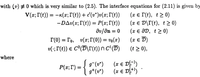
For agiven interface

$\mathrm{r}^{\ovalbox{\tt\small REJECT}}$, we

denote by $y)^{\ovalbox{\tt\small REJECT}}\ovalbox{\tt\small REJECT}_{\ovalbox{\tt\small REJECT}}$ )

and 7)$\ovalbox{\tt\small REJECT}^{+)}$ two components of $\mathrm{O}^{\ovalbox{\tt\small REJECT}}\ovalbox{\tt\small REJECT} \mathrm{Y}$, and let $\mathrm{p}(\mathrm{r}\ovalbox{\tt\small REJECT} \mathrm{I}^{\ovalbox{\tt\small REJECT}})$ stand for the unit

normal vecotor on $\mathrm{r}^{\ovalbox{\tt\small REJECT}}$ pointing into $\cdot\ovalbox{\tt\small REJECT}^{+)}$ (cf. Figure 1). The normal velocity $\mathrm{V}(\mathrm{r}\ovalbox{\tt\small REJECT} \mathrm{I}^{\ovalbox{\tt\small REJECT}}(\mathrm{f}))$

is always measured along $\mathrm{p}(\mathrm{r}\ovalbox{\tt\small REJECT} \mathrm{I}^{\ovalbox{\tt\small REJECT}}(\mathrm{f}))$

.

Here and in what follows, we always treat the

cases

$D$

FIGURE 1. $\Gamma$ divides $D$ into two parts, $D_{\Gamma}^{(-)}$ and $D_{\Gamma}^{(+)}$

.

where interfaces stay uniformly away from the boundary $\partial D$ ofdoamin.

From the standpoint of investigating the existence of equilibrium internal layer

solu-tions, it is natural to ask the next question:

If the interface equation (IE-f) has asmooth equilibrium solution $\Gamma$, then does

(1.1) have afamily of equilibriumsolutions with transition layerson $\Gamma$for small

$\epsilon>0$?

It turns out that the answerto this question is ratherdelicate. In [3], Fife and Greenlee

prove that the answer is affirmative if the condition

$\nabla_{x}c(x)|_{\Gamma}\cdot\nu(x, \Gamma)<0$ $x\in\Gamma$

is fulfilled, where $\Gamma$ is asmooth equilibrium solution of (IE-f), namely, $\Gamma=\{x\in$

$D|c(x)=0\}$ which, we suppose, is aclosed manifold of codimension 1. Moreover,

the solution thus obtained is astable equilibrium of (1.1). The equilibrium solution

$u(.x., \epsilon)$ has the following behavior for each $d_{0}>0$:

$\epsilon\varliminf_{0}?\mathit{1}(x., \epsilon)=\{\begin{array}{l}\phi^{(-)}(x)x.\in\overline{D_{\Gamma}^{(-)}}\backslash \Gamma^{(d_{0})}\phi^{(+)},(.\tau).\prime \mathrm{r}\in\overline{D_{\Gamma}^{(+)}}\backslash \Gamma^{(d_{0})}\end{array}$ uniformly,

where $\Gamma^{(d_{0})}$ stands for the $d_{0}$-neighborhood of $\Gamma$

.

It is of crucial importance to note that

the normal vector $\nu$ above is pointing into the regionwhere the solution $u$ assumes values

close to $\Phi^{(+)}$. Since _{$c(.\tau)\equiv 0$} on $\Gamma$, the condition above says that in the two regions away

from the interface $\Gamma$ the solution takes values close to absolute minima of the potential

$\mathrm{I}\prime \mathfrak{s}/-(u\tau\cdot.0)\dot{\prime}.’$.

On thc other hancl., it is also pointed out in [12], in the context of the

same

question

for asystem of reaction-diffusion equations, that if., on the other hand., the condition

$\nabla_{x}c(.\tau^{\tau})|_{\Gamma}\cdot\nu(x., \Gamma)>0$ $.\tau\cdot\in\Gamma$

(4)

is the case, then there may exist infinitely many internal laryer solutions which exhibit

sharp transitions near$\Gamma$

.

In radially symmetric

cases, the validity of the latter statement

has been established in [13]. By examining the proof in [12] and interpreting it in our

situation,

we can

state the following criterion on the existence of equilibrium internal

layer solutions.

Criterion 1: Let $\Gamma$ be asmooth equilibrium solution of (IE-f).

If it is

non-degenerate in the

sense

that the spectrum of the linearized operator

$L^{\mathrm{e}}\varphi$ $:= \epsilon(\Delta^{\Gamma}+\sum_{j=1}^{N-1}\kappa_{j}(x)^{2})\varphi+(\nabla_{x}c(x)|_{\Gamma}\cdot\nu(x, \Gamma))\varphi$ $x\in\Gamma$,

defined

on

$\Gamma$, isbounded away from

zero

uniformly in

$\epsilon\in(0, \epsilon\circ]$ forsome $\epsilon_{0}>0.$_,

then (1.1) has afamily ofsolutions with internal transition layer on $\Gamma$. In the

above, $\Delta^{\Gamma}$ is the Laplace-Beltrami

operator

on

$\Gamma$ and $\kappa_{i}(j=1, \ldots, N-1)$

stand for principal curvatures of$\Gamma$

.

Since $\Delta^{\Gamma}$ is anon-positive oprator, it

is apparent that if $\nabla_{x}c(x)|_{\Gamma}\cdot\nu(x, \Gamma)<0$then the

spectrum ofthe operator $L^{\epsilon}$ is

bounded away from

zero

uniformly in $\epsilon>0$. Hence the

criterion above is compatible with the result given by Fife and Greenlee [3].

Let

us

consider the following situation.

Al $I(x)\equiv 0$

on

$\overline{D}$, or

equivalently, $c(x)\equiv 0$ on $\overline{D}$

.

If Al is the case, there arises two kinds of degeneracy:

(1) Any closed

_manifold

$\Gamma\subset D$ ofcodimension one is an equilibrium of (IE-f)

(2) The corresponding linear operator $L^{\mathrm{e}}$ in the Criterion

1reduces to $\epsilon$ times the

Jacobi-0perator

on

$\Gamma$ and hence it has many small eigenvalues converging

to 0as

$\epsilonarrow 0$, making the criterion above powerless.

Therefore, we need first to establish aselection principle to identify possible equilibrium

interfaces.

Along the line of arguments employed in Nakamura et al. [6],

onc

can show that the

interface equation for (1.1) is given by

(1.6) $\mathrm{V}(x;\Gamma(t))=-\kappa(x;\Gamma(t))-\frac{\nabla_{\nu_{\Gamma}}n\iota(x)}{m(x)}.+\frac{\alpha(\tau)}{nl(\prime \mathrm{r})}.$

.

$x\in\Gamma(t)$, $t>0’$

.

where $\kappa(x;\Gamma)$ stands for the

sum

ofprincipal curvature of$\Gamma$ and

(1.6-a)

$nl(x)= \int_{-\infty}^{\infty}(\frac{\partial\tilde{Q}_{0}(\tau,x)}{\partial\tau}\cdot)^{2}cl\tau$ $x\in\overline{D}$ (unit transition momentum at

$.\tau\cdot$) $.$

,

(1.6-b)

$\alpha(x)=\int_{-\infty}^{\infty}f_{\epsilon}(\tilde{Q}\mathrm{o}(\tau;x), x, 0)\frac{\partial\tilde{Q}_{0}(\tau\cdot x)}{\partial\tau’}d\tau$ $x\in\overline{D}$ (

$\mathrm{e}\mathrm{x}\mathrm{c}\mathrm{e}\mathrm{s}\mathrm{s}- \mathrm{e}\mathrm{n}\mathrm{e}\mathrm{r}\mathrm{g}\dot{\mathrm{y}}$ of order $\epsilon$).

We

now

assume

that the following conditions are fulfilled.

A2 The interface equation (1.6) has asmooth equilibrium solution $\Gamma\subset D$.

(5)

A3 The equilibrium $\Gamma$ is non-degenerate in the sense that the linear operator

$A$ defined below does not have

0as

its eigenvalue:

(1.7) $A \varphi(.’\tau):=\uparrow?l(x)(\Delta^{\Gamma}+\sum_{j=1}^{N-1}\kappa_{j}^{\sim}(x)^{2})\varphi(x)+\nabla_{\Gamma}n\mathrm{z}(x)\cdot\nabla_{\Gamma}\varphi(x)$

$+(-\kappa(x;\Gamma)\nabla_{\nu_{\Gamma}}m(x)-\nabla_{\nu_{\Gamma}}^{2}m(x)+\nabla_{\nu_{\Gamma}}\alpha(x))\varphi(x)$ $x\in\Gamma$,

where $\nabla_{\Gamma}$ is the gradient operator on $\Gamma$

.

$1\mathrm{t}^{r}\mathrm{e}\mathrm{h}_{\dot{\epsilon}}\iota \mathrm{v}\mathrm{e}$:

Lemma 1.1. The operator $A$ is self-adjoint and its eigenvalues are all real:

(1.8) $\sigma(A)=\{\lambda_{j}\}_{j=0}^{\infty}\subset \mathbb{R}$, $\lambda_{0}>\lambda_{1}>\ldots>\lambda_{j}arrow-\infty$,

where only distinct eigenvalues are listed. The multiplicity

_of

$\lambda_{j}$ is denoted by $mj\geq 1$.

Let us now define afunctional $F(\Gamma)$ by

(1.9) $\mathrm{F}(\mathrm{T}):=\int_{\Gamma}m(x)dS_{x}^{\Gamma}-\int_{D_{\Gamma}^{(-)}}$ $a(x)dx$ $(\partial D_{\Gamma}=\Gamma’$

.

where $dS_{x}^{\Gamma}$ stands for the

surface

elementon $\Gamma$

.

Lemma 1.2. The Euler-Lagrange equation

_for

$F$ is given by

(1.10) $-\mathrm{k}(\mathrm{x};\Gamma)?n(x)-\nabla_{\nu_{\Gamma}}nl(x)+\alpha(x)=0$ $x\in\Gamma$,

and the second variation

_of

$F$ is described by

A9

defined

in (1.7).

Note that (1.10) is the equation for equilibrium solutions of theinterfaceequation (1.6).

Our main result is

Theorem 1.3 $([\overline{/}])$

.

Under the conditions Al, A2, and A3, there exist $\epsilon_{0}>0$ and $a$

family

_of

equilibrium solutions $u(x, \epsilon)$

of

(1.1),

defined for

$\epsilon\in(0., \epsilon_{0}]$, such that

for

each

$cl_{0}>0$

fixed

(1.11) $1\underline{\mathrm{i}\mathrm{n}}11l(.’\iota\cdot., \epsilon)=\epsilon 0\{$

$6^{(-)},(.\mathrm{z}\cdot)$

$x\in\overline{D_{\Gamma}^{(-)}}\backslash \Gamma^{(d_{\mathit{0}})}$

$o^{(+)}(:\iota.)$ $x\in\overline{D_{\Gamma}^{1+)}}\backslash \Gamma^{(d_{0})}$

uniformly,

where $D_{\Gamma}^{(\pm)}a7^{\cdot}\mathrm{C}$ tu)o regions _{$(\subset D)$} separated by$\Gamma$ and $\Gamma^{(\mathrm{r}l_{0})}$ stands

for

the $cl_{0^{-}}r\iota ei.qhborl\iota ood$

$()f\cdot\Gamma$.

Moreover,

_if

$\lambda_{0}<\mathrm{t}\mathrm{I}$ then $u(.’\iota\cdot\dot, \epsilon)$ is asymptotically stable, and

if

$\lambda_{k}$. $>0>\lambda_{k+1}$

for

sornc

$inte.c/C\mathit{7}^{\cdot}$$k\geq 0$ then it(.v

$\dot,$

$\epsilon$)is $ur\iota st‘\iota ble$ with instability index equal to $\sum_{j=0j}^{\mathrm{A}}.??l$.

Conclusion. Non-degenerate critical points of the functional $F$in (1.9)., if

reg-ular enough, give rise toequilibrium solutions of(1.1). The index of thc critical

point is equal to the dimension

_of

the unstable

_manifold

of the equilibrium

s0-lution. It is an amusing fact that the fornu$\iota \mathrm{l}\mathrm{a}\mathrm{e}$ $(1.6)$ and (1.7) naturally appear

in $11\mathrm{l}\dot{\mathrm{c}}\iota \mathrm{t}\mathrm{c}\mathrm{h}\mathrm{c}\mathrm{d}.\mathrm{a}\mathrm{s}\backslash ’ 1111$)totic expansions

(6)

The proof of Theorem 1.3 depends on the methods developed in $[13, 15]$ (matched

asymptotic expansions). When tie(x) $\equiv 1$ and $\alpha(x)\equiv 0$, the same result as Theorem 1.3

was first obtained by [5] for stable case, by using $\Gamma$

-convergence

and related variational

techniques. Our theorem extends those in [5] to cover unstable

cases.

Theorem 1.3

prompts the resolution of the following.

Geometric Variational Problem 1.

Find critical points of the functional F in (1.9).

We call this problem geometric because the unknown $\Gamma$ is ageometric object.

2. SYSTEM OF REACTION-DIFFUSION EQUATIONS

We now move on to deal with reaction-diffusion systems.

(2.1) $\{$

$\frac{\partial u}{\partial t}=\epsilon\Delta u-\frac{1}{\epsilon}f(u, v, \epsilon)$

$(x\in D, t>0)$ _,

$\frac{\partial v}{\partial t}=D\Delta v+g(u, v, \epsilon)$

$\frac{\partial u}{\partial \mathrm{n}}=0=\frac{\partial v}{\partial \mathrm{n}}$ $(x\in\partial D, t>0)$

.

The first equation in (2.1) looks almost identical to (1.1), ifwe replace $.’\iota$

.

in the latter by

$v(x)$

.

We assume in this section that the nonlinear term $f(u, x, \epsilon)$ is smooth and derived

from adouble-well potential $W(u, v, \epsilon)$:

(2.2) $f(u.v, \epsilon)’=\frac{\partial W(u,v,\epsilon)}{\partial u}$

with $u=h^{(\pm)}(v, \epsilon)$ denoting the locations of two wells, while $u=h^{(0)}(v, \epsilon)$ stands $\mathrm{t}1_{1}\mathrm{e}$

intermediate zero of$f(\cdot, v, \epsilon)$, satisfying

(2.2-a) $h^{(-)}(v, \epsilon)<h^{(0)}(v, \epsilon)<h^{(+)}(v, \epsilon)$ $v\in \mathbb{R}$

.

Similar to scalar case, the difference in the values of potential at the two wells will play

an

important role in describing the dynamics of (2.1). Let us denote the difference at

each $v$ by $J(v)$:

(2.3) $J( \mathrm{t}’):=\int_{h^{(-)_{(1’)}}}^{h^{(+)}}(v)f(u., v, \mathrm{O})du$.

$=\mathrm{T}\prime V(h^{(+)}(u), v.\mathrm{O})-\mathrm{t}\cdot V(h^{(-)}(v), v, 0)$

where $l\iota^{(\pm)}(v)=l\iota^{(\pm)}(\iota’, 0)$ (cf. (2.2-a)).

It is known [2] that the solution of (2.1) with appropriate initial conditions develops

transition layers in short timc., and that thc interface evolves according to the followin$\mathrm{g}$

(7)

system of interface equations:

(IE-a) $\mathrm{V}(.\tau.;\Gamma(t))=c(v(x,t))$ $(x\in\Gamma(t), t>0)$,

(IE-b) $v_{t}=D\Delta v+g^{\mathrm{x}}(v\dot,x;\Gamma(t))$ $(x\in D\backslash \Gamma(t), t>0)$,

(IE-c) $\partial v(x.,t)/\partial \mathrm{n}=0$ $(x\in\partial D, t>0)$,

(IE-d) $\Gamma(0)=\Gamma\circ$, $v(x, 0)=v_{0}(x)$ $(x\in D)$,

(IE-e) $v(\cdot,t)\in C^{1}(\overline{D})\cap C^{2}(D\backslash \Gamma(t))$

.

The function $g^{*}$ in (IE-b) is defined by

$g^{\mathrm{x}}(v, x;\Gamma(t))=\{$

$g^{-}(v)$ $:=g(h^{(-)}(v), v)$ if $x\in D_{\Gamma(t)}^{(-)}$

$g^{+}(v)$ $:=g(h^{(+)}(v), v)$ if $x\in D_{\Gamma(t)}^{(+)}$

.

The condidion in (IE-e) is called a $C^{1}$-matching condition.

It is also known [2] that the problem (IE) is well-posed and that its solutions do

ap-proximate the motion of the internal layer solutions of(2.1) on

_finte

time intervals $[0, T_{\epsilon}]$

(although $T_{\epsilon}arrow\infty$ as $\epsilonarrow 0$). Since for $\epsilon>0$ the approximation is valid only on finite

time intervals in general, some of asymptotic information on the solutions of (2.1) may

not be captured by only analysing the behavior of solutions of (IE-a,b,c,d). For example,

the results in [2] do not answer the following question:

If

$(\mathrm{I}\mathrm{E}- \mathrm{a}_{i}\mathrm{b},\mathrm{c}_{!}.\mathrm{d})$ has an equilibrium solution $(\Gamma_{0}, v(x;\Gamma_{0}))$, then, does (2.1) have

a corresponding equilibrium solutions

_for

small $\epsilon>0^{Q}$

The equilibrium solutions of (IE-a,$\cdot$b.c,d) have to satisfy

$0=c(v(x;\Gamma_{0}))$ $(x\in\Gamma_{0})$,

$0=D\Delta v+g^{\mathrm{x}}(v, x;\Gamma_{0})$ $(x\in D\backslash \Gamma_{0})$, $\partial v(x, \Gamma_{0})/\partial \mathrm{n}=0$ $(x\in\partial D)$

$v(\cdot;\Gamma_{0})\in C^{1}(\overline{D})\cap C^{2}(D\backslash \Gamma_{0})$

.

Let us denote by $v^{*}$ a zero _{$c(v):c(v^{\mathrm{x}})=0$}. Therefore, they are asolution of the following

free

boundary problem:

(FB-a) $0=D\Delta v+g^{\mathrm{x}}(v., x;\Gamma_{0})$ (x $\in D\backslash \Gamma_{0})$,

(FB-b) $v(x;\Gamma_{0})=v^{\mathrm{x}}$ on $\Gamma_{0}.$

, $\partial v(x;\Gamma_{0})/\partial \mathrm{n}=0$ on $\partial D$,

(FB-a) $v(\cdot;\Gamma_{0})\in C^{1}(\overline{D})\cap C^{2}(D\backslash \Gamma_{0})$

.

Note $\mathrm{t}1_{1}\mathrm{a}\mathrm{t}$ the nonlinearity_{$g^{\mathrm{x}}(v., x;\Gamma_{0}).$}

, in general, has jump discontinuity along $\Gamma_{0}$

.

The

free boundary problem can be reformulated as:

Find critical points $v(\cdot;\Gamma)$ of the functional $F(v;\Gamma)$:

$\mathcal{F}(v;\Gamma):=\int_{D}(\frac{1}{2}D|\nabla v|^{2}-G^{\mathrm{x}}(v, x,\cdot\Gamma))dx$

$( \mathrm{w}\mathrm{i}\mathrm{t}\mathrm{h}G^{\mathrm{x}}(v., \cdot\tau j.\Gamma):=\int_{v^{*}}^{v}g^{\mathrm{x}}(s, x;\Gamma)ds)$

.

Then identify $\Gamma_{0}$ so that $v(x.\cdot\Gamma_{0})\equiv v^{\mathrm{x}}$ on $\Gamma_{0}$.

(8)

For the sake of argument, let us assume that the free boundary problem $(\mathrm{F}\mathrm{B}- \mathrm{a}_{\ovalbox{\tt\small REJECT}}\mathrm{b}_{\ovalbox{\tt\small REJECT}}\mathrm{c})$ has

aregular solution $(\ovalbox{\tt\small REJECT}(\mathrm{x})\rangle’ \mathit{0})\ovalbox{\tt\small REJECT}$ Then it

was

shown in [12] that the linearized eigenvalue

problemdefined for $p(x)$ (rE$\mathrm{I}^{\ovalbox{\tt\small REJECT}}\mathrm{o})$and $q(\mathrm{r})$ (rE$\ovalbox{\tt\small REJECT} \mathrm{D})\ovalbox{\tt\small REJECT}$

(EVP4) $\lambda p=\epsilon(\Delta^{\Gamma_{0}}+\sum_{j=1}^{\mathit{1}\mathrm{V}-1}\kappa_{j}(x)^{2})p+c’(v^{*})\frac{\partial V^{*}(\tau)}{\partial\nu(x)}.|_{\Gamma_{0}}p+c’(v^{*})q|_{\Gamma_{0}}$ x $\in\Gamma_{0}$.

(EVP-2) $\lambda q=D\Delta q+g_{v}^{*}(V^{\mathrm{x}}(x),x;\Gamma_{0})q-[g^{*}]p\otimes\delta_{\Gamma_{0}}$ x $\in D$

plays

an

important role. In (EVP-I), $d(v^{*})$ is thederivative at $v=v^{\mathrm{r}}$of$c(v)$ with respect

to $v$

.

In (EVP-2), $[g^{*}]$ stands for the jump of$g^{\mathrm{x}}$ on $\Gamma 0$:

$[g^{*}]=g(h^{(+)}(v^{*}), v^{*})-g(h^{(-)}(v^{*}), v^{*})$,

and thesymbol $\delta_{\Gamma_{0}}$ stands for the Dirac-delta function supported

on

$\Gamma_{0}$

.

Therefore

(EVP-2) shouldbe interpreted indistributional

sense.

By writingit in weak form and integrating

by parts,

one can

recast (EVP-2)

as

concisely as

(EVP-2’) $\Pi_{\lambda}q|\mathrm{r}_{0}+[g^{*}]p=0$ x $\in\Gamma_{0}$,

where $\Pi_{\lambda}$ is the Dirichlet-t0-Neumann map defined by

$\Pi_{\lambda}q(x):=\Pi_{\lambda}^{-}q(x)+\Pi_{\lambda}^{+}q(x):=\frac{\partial v_{\lambda}^{-}(\prime\iota)}{\partial\nu(x)}.\cdot-\frac{\partial v_{\lambda}^{+}(x)}{\partial\nu(x)}$ $(x\in\Gamma_{0})$

in which $v_{\lambda}^{\pm}(x)$

are

solutions of the following problem:

$D\Delta v^{\pm}+g_{v}^{\mathrm{r}}(V^{\mathrm{x}}(x),x;\Gamma_{0})v^{\pm}=\lambda v^{\pm}$ $(x\in D_{\Gamma_{0}}^{(\pm)}, D_{\Gamma_{0}}^{(-)}\cup D_{\Gamma_{0}}^{(+)}=D\backslash \Gamma_{0})$

.

$v^{\pm}(x)=q(x)$ $(x\in\Gamma_{0})$,

$\frac{\partial v^{\pm}(x)}{\partial \mathrm{n}}=0$

$(x\in\partial D)$

.

Under the condition $g_{v}$

.

$<0$,

one

can show that $\Pi_{\lambda}$ is invertible for ${\rm Re}\lambda\geq-\lambda_{0}$ for some

$\lambda_{0}>0$

.

The following criterion has been established in [12].

Criterion 2Ifthe linear operator $A^{\epsilon}$, defined by

(L) $A^{\mathrm{e}}p:= \epsilon(\Delta^{\Gamma_{0}}+\sum_{j=1}^{N-1}f\dot{\iota}j(x)^{2})p+c’(v^{*})\frac{\partial V(!)}{\partial\nu(\tau)}..\cdot|_{\Gamma_{0}}p-c’(v^{\mathrm{x}})\Pi_{0}^{-1}p$ .x. $\in\Gamma_{0J}$.

is invertible uniformly in $\epsilon>0$, then (2.1) has afamily of equilibrium solutions

exhibiting transition layers

on

$\Gamma_{0}$

.

Note that this operator $A^{\epsilon}$ is obtained by

substituting (EVP-2’) with A $=0$ into (EVP-I).

When $c’(v^{*})<0$, it is in fact shown in [12] that the eigenvalues of (L) are $\mathrm{b}()\mathrm{u}\mathrm{n}(\mathrm{l}\mathrm{e}(1$

away from 0uniformly in $\epsilon>0$

.

If,

on

the other hand, $c’.(v^{\mathrm{x}})>0$ is the $\mathrm{c}\mathrm{a}\mathrm{s}.(^{\backslash },.$

, then the

opeartor $A^{\epsilon}$ has many small eigenvalues conveging to zero as _{$6arrow 0$}

.

(9)

$\backslash 1^{\gamma}\prime \mathrm{e}$denote by $(\tilde{Q}\mathrm{o}(\tau;v), c(v))$ the solution of (1.4) with

$x$, $\phi^{(\pm)}$, and $\phi^{(0)}$ begin replaced

by $\iota’.$

, $h^{(\pm)}(v).$, and $h^{(0)}(v)$

.

Similar to (1.5), $c(v)$ and $J(v)$ are related as

$J(v):=c(v) \int_{-\infty}^{\infty}(\frac{\partial\tilde{Q}_{0}(\tau,v)}{\partial\tau}\cdot)^{2}d.\tau$.

Let us now consider the following situation:

Bl $J(v)\equiv 0$ for $v\in \mathbb{R}$, or equivalently, $c(v)\equiv \mathrm{f}\mathrm{o}\mathrm{r}$ $v\in \mathbb{R}$

.

Under the condition Bl, the first equation (IE-a) decouples from others and the inter$\cdot$

face equations reduce to

$(\mathrm{I}\mathrm{E}- \mathrm{a}^{\dot{\prime}})$ $\Gamma(t)\equiv\Gamma\circ$ $(t\geq 0)$,

(IE-b) $v_{t}=D\Delta v+g^{\mathrm{x}}(v,$x;$\Gamma)$ (x $\in D\backslash \Gamma,$t $>0)$,

(IE-c) $\partial v(!.,t)/\partial \mathrm{n}=0$ $(x\in\partial D)$,

(IE-d’) $v(x., 0)=v\mathrm{o}(x)$ $(x\in D)$,

(IE-e) $v(\cdot, t)\in C^{1}(\overline{D})\cap C^{2}(D\backslash \Gamma)$

.

This equation is agradient system associated with the potential

$E(v) \equiv\int_{\mathcal{D}}(\frac{D}{2}|\nabla_{x}v(.\tau)|^{2}-G(v(x), x;\Gamma))dx$

(with

$G(v., x; \Gamma):=\int_{0}^{v}g^{\mathrm{x}}(s, x;\Gamma)ds$

),

and hence its solutions converge to an equilibrium solution as $tarrow\infty$.

In order to state our problem succinctly, let us define aset $S$ of interfaces.

(2.4) $S=\{\Gamma\subset D$ $|\Gamma$ is an $N-1$ dimensional, smooth, connected, $\mathrm{c}\mathrm{l}\mathrm{o}\mathrm{s}\mathrm{e}\mathrm{d}.\mathrm{m}\mathrm{a}\mathrm{n}\mathrm{i}\mathrm{f}\mathrm{o}\mathrm{l}\mathrm{d}\}$

.

Lemma 2.1. Under the condition Bl, assurne that

$\frac{l}{d_{1^{f}}}‘ g^{\pm}(v)<0$ $v\in \mathbb{R}$

.

$F_{CJ\mathit{7}}$. each $\Gamma\in S$, the problem

(BVP-I) $\{$

$0=D\triangle.v+g^{\mathrm{x}}(v., \cdot\tau j\Gamma)$ $(x\in D\backslash \Gamma)$

$\partial\iota,,(x)/\partial \mathrm{n}=0$ $(x\in\partial D)$

(BVP-2) $v(\cdot)\in C^{1}(\overline{D})\cap C^{-}’(D\backslash \Gamma)$

.

$l\iota as$ _$a$

Ulliclue

solution $\mathrm{t},’ \mathrm{r}(?\cdot)$.

$\backslash \backslash ^{\mathrm{v}}\prime \mathrm{e}$ encounter again adegenerate situation.

(1) Le mma 2.1 $\mathrm{S}_{I}^{\sigma}1.\backslash _{J}’.\mathrm{S}$ that under the condition Bl the interface equation

$(\mathrm{I}\mathrm{E}- \mathrm{a}.\mathrm{b}.\mathrm{c}_{\dot{l}}\mathrm{d})\prime\prime$ .

has

21 continuum ofequilibrium solutions $\{\tau_{\Gamma}’|\Gamma\in S\}$.

(2) $\wedge\backslash \mathrm{I}\mathrm{o}1^{\cdot}(^{\backslash }\mathrm{o}\backslash ^{\gamma}\mathrm{c}\mathrm{r}\dot,$ for each menbcr

$\mathrm{v}\mathrm{r}$ of the

$\mathrm{f}\dot{\epsilon}1\mathrm{n}1\mathrm{i}1\mathrm{y}_{\dot{\mathrm{r}}}$ thc operator $A^{\epsilon}$ does not satisfy the

$1^{\cdot}(^{\backslash }\prime \mathrm{c}1n\mathrm{i}\mathrm{r}\mathrm{e}1\mathrm{n}\mathrm{e}11\mathrm{t}$ in Criterion 2.

(10)

Therefore, under the condition Bl, the interface equations (IE-a,b,c,d) do not capture

essential dynamics of (2.1). To find arefined set of interface equations, we rescale time

and consider (2.1) in the following version:

(2.5) $\{$

$\frac{\partial u}{\partial t}=\Delta u-\frac{1}{\epsilon^{2}}f(u, v, \epsilon)$

$\frac{\partial v}{\partial t}=\frac{1}{\epsilon}(D\Delta v+g(u, v, \epsilon))$

$(.\tau. \in D, t>0)$

with the

same

boundary conditions as in (2.1).

Following the procedures employed in Nakamura et al. [6], one can show that the

interface equation for (2.5) is given by

(2.6) $\mathrm{V}(x;\Gamma(t))=-\kappa(x;\Gamma(t))-\frac{\nabla_{\nu_{\Gamma}}m(v_{\Gamma(l)})}{m(v_{\Gamma(l)})}+\frac{\alpha(v_{\Gamma(l)})}{1n(v_{\Gamma(l)})}$ _{$x\in\Gamma(t)$}, $t>0$,

where

(2.6-a) $nl(v)= \int_{-\infty}^{\infty}(\frac{\partial\tilde{Q}_{0}(\tau,v)}{\partial\tau}\cdot)^{2}d\tau$ $v\in \mathbb{R}$ (unit transition momentum at $v$),

(2.6-b) $\alpha(v)=\int_{h^{(-)}}^{h^{(+)}(v)}(v)f_{\epsilon}(u, v, \mathrm{O})du$ $v\in \mathbb{R}$ (excess-energy of order $\epsilon$).

The well-posedness of (2.6) has been established in [1].

We now assume that the following conditions are fulfilled.

B2 The interface equation (2.6) has asmooth equilibrium solution $\Gamma\in S$

.

B3 The equilibrium $\Gamma$ is non-degenerate in the

sense

that the linear operator

$B$ defined below does not have 0as its eigenvalue:

(2.7) $B \varphi(x):=nl(v_{\Gamma})(\Delta^{\Gamma}+\sum_{j=1}^{N-1}\kappa j(.\tau)^{2})\varphi(.\tau.)+\nabla_{\Gamma}rll(vr)$$\cdot$ $\nabla_{\Gamma}\varphi(x)$

$+(m’(v_{\Gamma}) \Delta^{\Gamma}v_{\Gamma}+\frac{/c^{+}(v_{\Gamma})+g^{-}(\uparrow 1\mathrm{r})}{2D}-m’(v_{\Gamma})|\nabla_{\nu_{\Gamma}}v_{\Gamma}|^{2}+\nabla_{\nu_{\Gamma}}\alpha(\iota_{\Gamma},,))\varphi$

$+ \frac{[g]}{D}.(-\kappa(x;\Gamma)m’(v\mathrm{r})-nl’(v\mathrm{r})\nabla_{\nu_{\Gamma}}v_{\Gamma}+\nabla_{\nu_{\Gamma}}\alpha(v\mathrm{r}))\Pi_{0}^{-1}\varphi(.\tau)$

$+ \cdot\frac{[c/]}{D}.\frac{r1l’(v_{\Gamma})}{2}(\Pi_{0}^{-}-\Pi_{0}^{+})\Pi_{0}^{-1}\varphi(.\tau)$ _$x\in\Gamma$,

where

$g^{\pm}(v)=g(h^{(\pm)}.(\cdot\iota’), v)$

.

Although the operator $B$ looks quite complicated, it enjoys the following property.

Lemma 2.2. The operator$B$ is self-adjoint and its eigenvalues are all real:

(2.8) $\sigma(B)=\{\lambda_{j}^{s}\}_{j=0}^{\infty}\subset \mathbb{R}$, $\lambda_{0}^{s}>\lambda_{1}^{s}>\ldots>\lambda_{j}^{s}arrow-\infty_{\dot{l}}$

where only distinct eigenvalues are listed. The multiplicity

_of

$\lambda_{j}^{s}$ is denoted by ’}$\iota_{j}^{\mathit{8}}\geq 1$.

(11)

Remark 2.3. The operator $B$ is self-adjoint only when the interface $\Gamma\in S$ is connected.

If $\Gamma$ has more than one connected components, the operator $B$ may not be self-adjoint.

Let us now define afunctional $F_{s}(\Gamma)$ by

(2.9) $F_{s}( \Gamma):=\int_{\Gamma}m(v_{\Gamma})d.S_{x}^{\Gamma}-\int_{D_{\Gamma}^{(-)}}\alpha(v_{\Gamma})dx$,

where $v_{\Gamma}$ is the solution given in Lemma 2.1.

Lemma 2.4. The Euler-Lagrange equation

_for

$F_{s}$ is given by

(2.10) $-\kappa(x;\Gamma)m(v_{\Gamma})-\nabla_{\nu_{\Gamma}}m(v_{\Gamma})+\alpha(v_{\Gamma})=0$ $x\in\Gamma$,

and the second variation

_of

$F_{s}$ is described by $B\varphi$

defined

in (2.7).

Our main result for system (2.1) is:

Theorem 2.5. Under the conditions Bl, B2, and B3, there eist $\epsilon\circ>0$ and a family

of

equilibrium solutions $(u(x, \epsilon)$,$v(x, \epsilon))$

of

(2.1),

defined for

$\epsilon\in(0, \epsilon\circ]$, such that

for

each

$d_{0}>0$

fixed

$\varliminf_{\epsilon 0}v(x_{\dot{J}}\epsilon)=v_{\Gamma}(x)$

unifo

rmly on

$\overline{D}.$

,

$\varliminf_{0}u(x, \epsilon)=\{\begin{array}{l}h^{(-)}(v_{\Gamma}(x))h^{(+)}(v_{\Gamma}(x))\end{array}$ uniformly on $\{$

$\overline{D_{\Gamma}^{(-)}}\backslash \Gamma^{(d_{0})}$

$\overline{D_{\Gamma}^{(+)}}\backslash \Gamma^{(d_{0})}$

where $D_{\Gamma}^{(\pm)}$ are two regions _{$(\subset D)$} separated by$\Gamma$ and $\Gamma^{(d_{0})}$ stands

for

the $d_{0}$-neighborhood

of

$\Gamma$.

Moreover, the eigenvalues

_of

$B$ determine the stability

of

the equilibrium solutions:

$\bullet$

If

$\lambda_{0}^{s}<0$, then the solution is asymptotically stable.

$\bullet$

If

$\lambda_{k}^{s}$. _{$>0>\lambda_{k\cdot+1}^{s}$}

for

some integer$k\geq 0$, then the solution is unstable withinstability index equal to $\sum_{j=0}^{\mathrm{A}}.m_{j}^{s}$.

This theorem makesit meaningful toestablish some methodsto deal with the following

problem.

Find critical points of the functional $F_{s}$ in (2.9).

Remark 2.6. Even if the interface $\Gamma$ has more than one connected components, the

state-mcnt of Theorem 2.5 is still $\backslash ^{\gamma}\mathrm{a}1\mathrm{i}\mathrm{d}.$

, except for the stability properties. In such asituation,

thc operator $B$ is not self-adjoint and may have complex eigenvalues. $\mathrm{M}_{\wedge}\mathrm{o}\mathrm{r}\mathrm{e}\mathrm{o}\mathrm{v}\mathrm{e}\mathrm{r}.$

,

consid-ering the diffusion coefficient $D$ as abifurcation parameter, one may be able to detect

Hopf-bifurcations of interfaces. In $\mathrm{f}\mathrm{a}\mathrm{c}\uparrow.$

, it is confirmed in [14] that the Hopf-bifurcation

of interfaces can occur in the following system

(2.11) $\{$

$\frac{\partial u}{\partial t}=\Delta u-\frac{1}{\epsilon^{\underline{)}}}.f(u.v.\epsilon)$ \prime\prime

$.. \frac{\partial\tau\prime}{\partial t}=\frac{1}{\epsilon}(\frac{D}{\epsilon}\Delta v+g(u’.v_{\dot{l}}\epsilon))$

$(.\tau\in D, t>0)$

(12)

with $(v)\not\equiv \mathrm{O}$ which is very similar to (2.5). The interface equations for (2.11) is given by $\mathrm{V}(x;\Gamma(t))=-\kappa(x;\Gamma(t))+c’(v^{\mathrm{x}})v(x;\Gamma(t))$ $(x\in\Gamma(t), t\geq 0)$

$-D\Delta v(x;\Gamma(t))=P(x;\Gamma(t))$ $(x\in D\backslash \Gamma(t), t\geq 0)$ $\partial v/\partial \mathrm{n}=0$ _{$(x\in\partial D, t\geq 0)$}

$\Gamma(0)=\Gamma\circ$, $v(x;\Gamma(0))=v\mathrm{o}(x)$ $(x\in\overline{D})$ $v(\cdot;\Gamma(t))\in C^{2}(\overline{D}\backslash \Gamma(t))\cap C^{1}(\overline{D})$ $(t\geq 0)$,

where

$P(x;\Gamma)=\{$

$g^{-}(v^{*})$ $(x\in D_{\Gamma}^{(-)})$ $g^{+}(v^{*})$ $(x\in D_{\Gamma}^{(+)})$

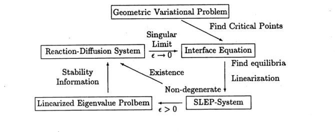
In aseriesof works [8, 9, 10, 11] on

one

dimensionalreaction-diffusionsystems, Nishiura

and his $\mathrm{c}\mathrm{o}$-workers have established apowerful method called the Singular Limit

Eigen-value Problem method (SLEP-method, for short) to determine the stability property of

equilibrium transition layer solutions. The basic structure of the method is concisely

expressed in the following diagram.

FIGURE 2. Relationship between reaction-diffusion system and SLEP-system.

First construct

an

equilibrium transition layersolution to the reaction-diffusion system

and linearize the system around it to obtain

an

eigenvalue problem. The singular limit

ofthe eigenvalue problem is called the SLEP-system which contains full information on

the stability of the equilibrium. Moreover, Nishiura et al. show that the SLEP-system

is also obtained by first passing to the singular limit of the reaction diffusion system to

obtain

an

associated system of interface equations and then linearizing the latter around

its equilibrium.

Our results fit pricisely into the

same

framework. We first find

an

equilibrium to the

systemofinterfaceequations and linearize it to obtain aSLEP-system. Then our assertion

is that if the SLEP-system thus obtained is non-degenerate, then the equilibrium of the

system of interface equations gives rise to an equilibrium transition layer solution of the

reaction-diffusion system. Moreover, the SLEP-systemalso carries the full$\inf_{0\Gamma 111}\mathrm{a}\mathrm{t}\mathrm{i}()\mathrm{n}$ on

the stability ofthe transition layer solution. We also point out the following facts which

are

guiding principles in

our

proof.

$\bullet$ The interface equations

are

nothing but thc lowest order

$C^{1}- \mathrm{m}\mathrm{a}\mathrm{t}\mathrm{c}1_{1}\mathrm{i}\mathrm{n}\mathrm{g}$ conditions

(13)

\bullet The

_SLEP-s.v

stem is the principal part of the higer order $C^{1}$-matching conditions.

FIGURE 3. Non-degenerate equilibra of the interface equations give rise

to transition layer solutions of reaction-diffusion system and their stability

properties are completely determined by SLEP-system.

3. OUTLINE OF _Proof

The proofconsists ofthree steps:

(1) Construction ofhighly accurate approximate solutions $U_{\mathrm{a}\mathrm{p}\mathrm{p}}^{arrow\epsilon}$ via the method

ofmatched asymptotic expansion. The conditions A2 ancl A3 (resp. B2 and B3)

allow us to find $C^{1}$-matched approximate solutions with arbitrarily high order of

accuracy. As pointed out at tlie end of the previous section, A2 (B2) is the lowest

order $C^{1}$-matchingcondition, and A3 (B3) allowusto find higher order$C^{1}$-matched

approximations. Once an approximate solution is constructed, the original problem

is then $\mathrm{W}\mathrm{l}\cdot \mathrm{i}\mathrm{t}\mathrm{t}\mathrm{e}\mathrm{n}$ as

(3.1) $\mathcal{L}^{\epsilon_{\acute{\mathrm{Y}}^{\hat{\prime}}}}+N^{\epsilon}(\varphi)+\mathcal{R}^{\epsilon}=0_{\dot{\mathit{1}}}$

where

_C’9

is obtained from the original problem by linearization around the

approx-make solutions $N^{\epsilon}(\varphi)$ stands for nonlinear terms containing quadratic and higer

order $\mathrm{t}\mathrm{e}\mathrm{l}\cdot \mathrm{l}\mathrm{n}\mathrm{s}$in

$(_{\hat{\prime}}.$, and 72’ measures how well the approximation satisfies the original

proble$\mathrm{m}$.

(2) The spectral analysis of$\mathcal{L}^{\mathrm{e}}$. The linearoperator$\mathcal{L}^{r}$ ingeneral has small eigenvalues

that go to zero as $\epsilonarrow 0$. called critical eigenvalues. In the present $\mathrm{s}\mathrm{i}\mathrm{t}\mathrm{u}\mathrm{a}\mathrm{t}\mathrm{i}\mathrm{o}\mathrm{n}_{\dot{J}}$ these

critical eigenvalues are of order $O(\epsilon^{2})$. and when divided by $\epsilon^{2}$ they are essentially

the eigenvalues of the SLEP-system. $\mathrm{T}\mathrm{h}\mathrm{e}\mathrm{r}\mathrm{C}^{\backslash }\mathrm{f}\mathrm{o}\mathrm{r}\mathrm{e}\dot,$ A3 (B3) guarantees that thc linear

operator $\mathcal{L}^{c}$ is invertible, although it has small eigenvalues that converge tozero as

$\epsilon$ $arrow 0$.

(3) To establish the solvability of (3.1). Since the linear part $\mathcal{L}^{\epsilon}\varphi$ is small $O(\epsilon^{2}).$

,

one needs to make the contribution of the nonlinear term $N^{\epsilon}(_{\hat{r}}\backslash ’)$ smaller than the

linear part. This., in turn, _{is possible if the} remainder term $\mathcal{R}^{e}$ is small

enough.”say,

$||\mathcal{R}^{\epsilon}||=O(\epsilon^{8})$ in the present situation. Thus one obtains the true solution

$U^{\epsilon}$ very

close to thc approximate one. Now thc linearization of thc original problem around

the genuine solution $U^{-\epsilon}$ is avery small perturbation of $\mathcal{L}^{\epsilon}.$

, and hcnce the stability

(14)

properties of U’is completely determined by the SLEP-system which has already

been analized in the previous Step (2).

The stragegy descirbed above

seems

to have awide

range

of applicability in dealing

withtransition layers and interfaces. The

same

idea has bccn successfully applied in other

situations $[4, 15]$

.

REFERENCES

[1 A. Bonami, D. Hilhorst, E. Logak and M. Mimura, Singular limit _ofa chemotaxis-growth m.odel,

Preprint 1999.

[2] X-F. Chen, Generation and propagation _{of interfaces} in _{reaction-diffusion} systems, Trans. $\mathrm{A}.\backslash$IS,

334(1992), $87\overline{/}- 913$

.

[3] P.C. Fifeand W.M. Greenlee, _{Interior transition layers}_from _{elliptic boundary value}_{problems with}

a smallparameter, Russian Math. Surveys, 29(1974), No. 4, _103-131.

[4] T. Iibun and K. Sakamoto, Internal layers intersecting the boundary _ofdomain in the Allen-Cahn Equation, Preprint 2000 (to appear in J. J. Ind. Appl. Mathemathics).

[5 It. V. Kohn and P. Sternberg, Local minimisers and singular perturbations, Proc. Royal Soc.

Edin-burgh, lllA(1989), 69-84.

[6] K.-I. Nakamura, H. Matano, D. Hilhorst, and R. Schitzle, Singular Limit _ofa _{Reaction-Diffusion}

Equationwith a Spatially Inhomogeneous Reaction Tem, J. Stat. Phys., 95(1999),1165- 1184.

[7] $\mathrm{N}.\backslash !^{\mathrm{T}}$

.

Nefedov and K. Sakamoto,

Multi-Dimensional Stationary Internal Layers_for Spatially

InhO-mogeneous_{Reaction-Diffusion} Equations with Balanced Nonlinearity, In preparation.

[8] Y. Nishiura, Coexistence _ofinfintely many stable solutions to reaction _diffusion systems in the sin-gular limit, Dynamics Reported, $3(1994)$, 25-103.

[9] Y.Nishiura, _{Nonlinear Problems 1–Mathematics}_for_{Pattern Formation-, Vol. 7Iwanami Series}

on Developments of Modern Mathematics, Tokyo 1998.

[10] Y. Nishiuraand H. Fujii, Stability _ofsingularly perturbed solutions to reaction _diffusion equations,

SIAMJ. Math. Anal. 18(1987)m 1726-1770.

[11] Y. Nishiura and M. Mimura, Layer oscillations in _{reaction-diffusion}systems, SIAMJ. Appl. Math. 49(1989),481-514.

[12] K. Sakamoto, Internal layers in high-dimensional domains, Proc. Royal Soc. Edinburgh,

$128\mathrm{A}(1998)$, 359-401.

[13] K. Sakamoto, _{Bifurcation of}infinetely many _fine modes _from radially symmetric internal layers,

Preprint (1999).

[14] K. Sakamoto, _Interface_Equations _with _{Nonlocal Effects,} _Preprint _2000.

[15] K. $\mathrm{S}\mathrm{a}\mathrm{k}$

-amoto and H. Suzuki, _{Symmetry breaking}_from _radially _symmetric _{internal layers,} _Preprint

(1999).