Stability Analysis of Numerical Solution of Stochastic Differential Equations(2nd Workshop on Stochastic Numerics)

Stability Analysis

of Numerical

Solution

of

Stochastic

Differential

Equations

三井

斌友

Taketomo

MITSUI*

名古屋大学人間情報学研究科

Graduate

School

of Human Informatics,

Nagoya

University,

Nagoya

464-01,

Japan

$\mathrm{e}$

-mail: [email protected]

1

Introduction

Our present aim is to show a linear stability analysis of numerical solution of stochastic differential equations (SDEs). As in other areas of numerical analysis, $n$umerical $sta$bility is significant in the case of SDEs which usually require a long (numerical) time-integration.

We will take the viewpoint how the analysis for SDEs is similar to as well as different from that for ordinary differential equations (ODEs), for the corresponding theory has been well

developed in the ODE case. On the contrary stability analysis for numerical schemes of

SDEs is still in a premature stage, although much work has been devoted to it. Here some previous trials for analytical and numerical

_stability,

concept in

SDEs

will be arranged to clear their interrelationships.

1.1

Stochastic

initial-value problems

We are concerned with the initial-value problem (IVP) of

SDE

ofIt\^o-type given as follows.

$\{$

$dX(t)=f(t,X(t))dt+g(t,X(\iota))dW(t)$ $(t>0)$,

$X(t)=X_{0}$, initial condition. (1.1)

Here $W(t)$ stands for the standard Wiener process. Under appropriate assumptions for the functions $f$ and $g$, the solution $X(t)$, as a random process, of IVP (1.1) is known to exist in the It\^o sense. Sincemany phenomena in scienceand engineering can be formulated with IVP ofSDEs and the problems are often not known to have analytical solutions, numerical

solutions turn out $.\mathrm{t}\mathrm{o}$ be practically important, and

have.been

$\mathrm{d}\mathrm{e}\dot{\mathrm{v}}\mathrm{e}1_{0}\mathrm{p}\mathrm{e}\mathrm{d}$ for the last decade.

Its

state-of-the-art

can be found in $e.g$

.

$[8]$

.

1.2

Syntax

diagram of stability

For theanalysis ofnumericalstabilityofdifferential equations, itsdistinctionandrelationship

with the stability of the underlying differential equation is considered to be crucial. Hence,

after LAMBERT $([12], \mathrm{P}^{3}8)$, we introduce a syntax diagram of stability.

Consider

IVP of ODEs given by

$\frac{dy}{dt}=f(t, y)$ $(t>0)$, $y(\mathrm{O})=y_{0}$, (1.2)

and its numerical (discrete variable) solution $\{y_{n}(n=0,1, \ldots)\}$ with a fixed stepsize $h$ and

step-points $\{t_{n};t_{n}=nh\}$ in the usual manner.

A stability definition can be broken down into the following components:

1. We impose certain conditions $C_{p}$ on (1.2) which force the exact solution $y(t)$ to display a certain stability property.

2. We apply a numerical method to the problem, assumed to satisfy $C_{p}$

.

3. We ask what conditions$C_{m}$ must be imposed on themethod in order that the numerical

solution displays a stability property analogous to that displayed by the exact solution. The components and the process can be readily understandable through a diagram shown

as in Fig. 1.1.

Figure 1.1:

Generic

syntax diagram of stability

In this way, the syntax diagram for zero-stability of numerical solution

can

be

written

([12]) as in Fig. 1.2.

More important concept is $A$-stability. When a linear system of ODEs

$\frac{dy}{dt}=Ay$, (1.3)

is considered with a $d$-dimensional matrix $A$, the asymptotic stability of the solution, $i.e.$,

$||y(t)||arrow 0$ as $tarrow\infty$,is expected to hold with acertain normof vectors. Its counterpart

innumerics is absol$\mathrm{u}te$stability. Byintroducing theregionof absolutestability,

$\mathcal{R}$, ofa linear

multistep or Runge-Kutta method ([3]), the syntax diagram of absolute stability is given by

Fig.

1.3.

As can be seen, the absolute stability depends on the magnitude of the stepsize

$h$

.

A method is called $A$-stable if it is absolutely stable for any $h$

.

Taking the asymptotic

stability of the underlying ODE system into account, $A$-stability can be said to be a kind of

ideal concept of stabilityin numerical ODEs. However, many barriers areknown for A-stable numerical schemes in ODEs ([4]).

Figure 1.2: Syntax diagram of zero-stability

Figure

1.3:

Syntax diagram of absolute stability

1.3

Carrying over

to SDE

To carry over the usefulness of$\mathrm{n}\mathrm{u}\mathrm{m}\mathrm{e}\mathrm{r}\mathrm{i}_{\mathrm{C}\mathrm{a}1}\sim$stability analysis to SDE case, the following

ques-tions should be resolved in turn:

”

Ql. What kind of stability concept is adopted in (analytic) SDE?

Because ofits statistical nature, $\mathrm{I}\mathrm{V}.\mathrm{P}$ of

SDEs

is followedby plenty conceptsofstability

([5]).

Q2. What is the condition or criterion of stability? It corresponds to $C_{p}$ in Fig. 1.1.

’1it..,$\backslash \triangleright$

Q3. What scheme is to be considered in numerical SDE? $\mathfrak{t}$

Variousnumerical schemes have beenproposedfor

SDEs.

As wewill seelaterin

Section

5, in some cases we must pay attention to the realization means of approximation of

the increment of the Wienerprocess with respect to the numerical stability.

Q4. What is the stability concept in numerical

SDE?

Q5. What is the condition or criterion of numerical stability? It corresponds to $C_{m}$ in Fig. 1.1.

2

Stochastic

stability

Here we will briefly describe how the stability concept is introduced into SDEs. Then the first trial is given for a syntax diagramof stability. However, we will seea nalve\simintroduction

cannot get a success.

2.1

Introduction

of

stochastic

stability

As in (1.1), consider a scalar It\^o-type SDE

$dX(t)=f(t,X(t))dt+g(t,x(t))dW(t)$ $(t>t_{0})$,

together with a nonran$dom$ initial value $X(t_{0})=x_{0}$

.

We assume that there exists a unique

solution $X$($t;$to,$x_{0}$) of the equation for $t>t_{0}$

.

Some

sufficient conditions have been

estab-lished for the unique existence of the solution. Moreover, we suppose that the equation allows a steady solution $X(t)\equiv 0$

.

This means the equation $f(t,0)=g(t,0)=0$ holds. A

steady solution is often called an equilibrium position.

$\mathrm{H}\mathrm{A}\mathrm{S}’ \mathrm{M}\mathrm{I}\mathrm{N}\mathrm{s}\mathrm{K}\Pi([5])$gave the following three definitions of stability.

Definition

2.1 The equilibrium position

_of

the $SDE$ is said to be stochastically stable

iffor

all positive $\epsilon$ and

for

all $t_{0}$ the equality

$\lim_{x0arrow 0}P(\sup_{t\geq t\mathrm{o}}|X$($t;$to,$x_{0}$)$|\geq\epsilon)=0$ holds.

Definition 2.2 The equilibrium position is said to be stochastically asymptotically stable if, in addition to the above condition in

_Definition

2.1, the equality

$\lim_{x\mathrm{o}arrow 0}P(\lim_{t\vee\infty}|X(t;t_{0,0}x)|=0)=1$

holds.

Definition

2.3 The equilibrium position is said to be stochastically asymptotically stable in

the large if, moreover to the above two conditions, the equality

$P( \lim_{tarrow\infty}|X(t;t0, x_{0^{)1}}=0)=1$,

for

all $x_{0}$

holds.

Definitions 2.1, 2.2 and

2.3

can be seen as the counterparts ofstability, asymptotic stability

and asymptotic stabilityin the large, respectively, in the

ODE

case. Henceforththeycan be

Actually we can derive a criterion of the asymptotic stochastic stability for the SDE. Assume that the functions $f$ and $g$ are uniformly asymptotically linear with respect to $x$, that is to say, for certain real constants $a$ and $b$the equations

$f(t,x)=ax+\overline{f}(t, x)$ and $g(t,x)=b_{X}+\overline{g}(t,x)$

hold with

$|x| arrow 01\mathrm{i}\mathrm{n}\frac{|\overline{f}(t,X)|+|\overline{g}(t,X)|}{|x|}=0$

uniformly in $t$

.

The solution $X(t)$ of the

SDE

is stochastically asymptotically stable if the

condition

$a- \frac{1}{2}b^{2}<0$ (2.1)

holds (see [2], p139).

This criterion strongly suggests a possibility of analogous linear $st\mathrm{a}$bility analysis for

numerical schemes of

SDE

to those of ODE. We can consider that the linear parts of$f$ and

$g$ are dominant in the asymptotic behaviour ofsolutions around the equilibrium position.

2.2

Numerical stability along

stochastic

stability

Following the suggestion in the previous subsection, we introduce a linear test equation (supermartingaleequation)

$dX(t)=\lambda X(t)dt+\mu X(t)dW(t)$ $(t>0)$ (2.2) with the initial condition $X(\mathrm{O})=1$ to the numerical stability analysis. Here $\lambda$ and

$\mu$ are

complex numbers.

Since the exact solution of (2.2) is written as

$X(t)= \exp\{(\lambda-\frac{1}{2}\mu^{2})t+\mu W(t)\}$,

it is quite easy toshowthat the equilibriumposition$X(t)\equiv 0$isstochasticallyasymptotically

stable if the condition

$\Re(\lambda-\frac{1}{2}\mu^{2})<0$ (2.3)

holds. In ourmind we employ the condition which can stand for $C_{p}$ in the syntax diagram.

A typical example of numerical scheme is the Euler-Maruyamascheme given as follows.

Let $h$ be the stepsize of the variable $t,$ $t_{n}=nh,$$(n=1,2, \cdots)$ the step-points, and

$\triangle W_{n}=W(tn+1)-W(t_{n})$

theincrement of the Wiener process at the n-th step-point. For the equation (1.1) the scheme

generates a discrete random process $\{X_{n}\}$ according to the recurrence

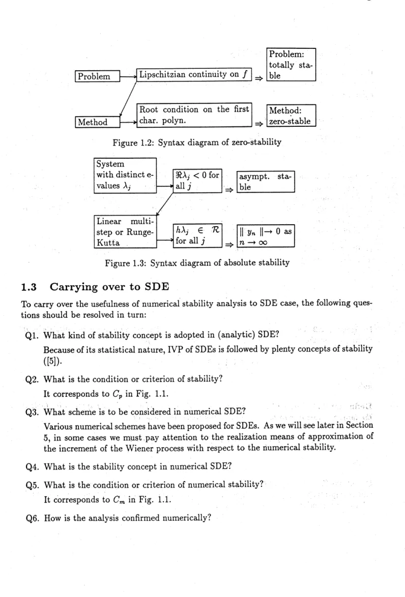
Figure 2.1: A syntax diagram?

The increment $\Delta W_{n}$ will be realized with certain normal random numbers with mean $0$ and

variance $\sqrt{h}$

.

Thus we think of a syntax diagram shown in Fig. 2.1.

However, this syntax diagram does not work well. The reason follows. The criterion

(2.3) for the stochastic asymptotic stability of (2.2) allows the cas$e\Re\lambda>0$

.

It implies that

some sample paths of the solution surely decrease to $0$, whereas their distributions possibly increase. This can be understood through the fact that when $\Re\lambda>0$ the equation cannot

be asymptotically stable even in the ODE sense. Henceforth it is impossible to carry out a numerical scheme until all the sample paths of the exact solution diminish to $0$ if two

conditions $\Re\lambda>0$ and $\Re(\lambda-\frac{1}{2}\mu^{2})<0$ are valid simultaneously. Since the numerical

solution by $e.g$

.

the Euler-Maruyama scheme would reflect this statistical property, nobody

can expect a numerically stable solution.

This investigation implies the necessity of another stability concept for

SDEs.

That is, we try to answer the question what SDE is having all sample paths whose distribution tends to $0$ as $tarrow\infty$.

3

MS-stability

Analysis of the previous section suggests an introduction of norm of the SDE solution with

respect to the stability concept.

3.1

Asymptotic

stability

in

$r\mathrm{t}\mathrm{h}$

mean

Return to the general IVP of

SDE

given in (1.1):

$dX(t)=f(t, X(t))dt+g(t,X(t))dW(t)$ $(t>t_{0})$, $X(t_{0})=X0$

.

Definition 3.1 The steady solution $X(t)\equiv 0$ is said to be $a\mathit{8}ymptoti_{Cal}ly$ stable in p-th

mean

_{if for}

all positive $\epsilon$ there exists a positive

$\delta$ which

satisfies

$\mathrm{E}(|X(t)|^{p})<\epsilon$

for

all $t\geq 0$ and $|x_{0}|<\delta$ (3.1)

and,

_{furthermore if}

there exists a positive $\delta_{0}$ satisfying

Here $\mathrm{E}mena\mathit{8}$ the mathematical expectation.

Roughly speaking, by the asymptotic stability in p-th mean we expect the asymptotic

di-minishing ofthe solution in the p-th moment.

The case of $p=2$ is most frequently used $\mathrm{a}\mathrm{n}\mathrm{d}\wedge$ called the mean-square case. Thus we

introduce the norm of the solution by

$||X||=\{\mathrm{E}|x|^{2}\}^{\frac{1}{2}}$

.

The necessary and sufficient condition is given in the following.

Lemma 3.1 The linear test equation (supermartingale equation) (2.2) with the unit initial value is $a\mathit{8}ympt_{\mathit{0}}tiCally$ stable in the mean-square sense

iff

the inequality

$2\Re\lambda+|\mu|^{2}<0$

holds.

Proof.

For the solution $X(t)$ of (2.2) with the unit initial condition, its mean-square $\mathrm{Y}(t)=$

$\mathrm{E}|X(t)|^{2}$ satisfies an IVP of ODE

$dY=(2\Re\lambda+|\mu|^{2})Ydt$ $(t>0)$, $\mathrm{Y}(\mathrm{O})=1$

.

The solution is obviously asymptotically stable when the inequality holds, and vice versa. $\square$

Note that since the $\mathrm{i}\mathrm{n}\mathrm{e}\mathrm{q}\mathrm{u}\mathrm{a}\mathrm{l}\mathrm{i}\mathrm{t}\mathrm{y}.\Re(2\lambda-\mu)2\leq 2\Re\lambda+|\mu|^{2}$ is always valid, the asymptotic

stability in the mean-square sense implies the stochastic stability.

In the sequel, the stability in the mean-square sense willbe abbreviated as $MS- \mathrm{s}\mathrm{t}\mathrm{a}\mathrm{b}\mathrm{i}1_{\hat{1}\mathrm{t}\mathrm{y}}$

.

3.2

Numerical

MS-stability

For asymptotically $MS$-stable problems of SDEs, what conditions are imposed to derive numerically asymptotically $MS$-stable solutions? That is to say, what conditions should be

for the numerical solution $\{X_{n}\}$ of the linear test equation (2.2) to achieve $||X_{n}||arrow 0$ as $narrow\infty$

.

Denote $\mathrm{E}|X_{n}|^{2}$ by $\mathrm{Y}_{n}$

.

When we apply a numerical

schenie

to the linear test equation and

take the mean-square norm, we obtain a one-step difference equation of the form

$\mathrm{Y}_{n+1}=R(\overline{h}, k)Y_{n}$ (3.3)

where two scalars $\overline{h}$

and $k$ stand for $h\lambda$ and $\mu^{2}/\lambda$

,

respectively. We

can

call $R(\overline{h}, k)$ the

stability function of the scheme, for the $MS$-stability of the numerical scheme is subject to its magnitude. That is, the equivalence

$\mathrm{Y}_{n}arrow 0$ as $narrow\infty\Leftrightarrow|R(\overline{h}, k)|<1$ holds.

Figure 3.1: Syntax diagram of MS-stability

Definition 3.2 ([14]) The scheme is said to be $MS$-stable

for

$\overline{h}$ and _$k$

if

its stability

func-tion $R(\overline{h}, k)$ is less than unity in magnitude. The set in $C^{2}$ given by

$\mathcal{R}=$

{

$(\overline{h},$$k);|R(\overline{h},$ $k)|<1$

holds}

is called the domain

_of

$MS$-stability

of

the scheme. The syntax diagram of $MS$-stability is in Fig. 3.1.

To compare the stability performance of various numerical schemes, we are to draw their figures. However, the complex values $\lambda$ and

$\mu$ yield the pair $(\overline{h}, k)$ in

four

dimensions! We

have to restrict ourselves to the case of real values of $\lambda \mathrm{a}\mathrm{n}\mathrm{d}/\mathrm{o}\mathrm{r}\mu$ for viewing the figures.

In addition, we can say that a numerical scheme is $A$-stable ifit is _$MS$-stable for any $h$

.

3.3

Stability function of

some

schemes

We will derive the stability function of some numerical schemes known in the literature. Details with figures will appear in [14].

First is the Euler-Maruyama scheme (2.4), whose application to (2.2) implies

$X_{n+1}=X_{n}+h\lambda X_{n}+\mu X_{n}\Delta W_{n}$

.

We obtain the stability function as

$R(\overline{h}, k)=|1+\overline{h}|2+|k\overline{h}|$

.

Fortunately the function depends on $\overline{h}$

and $|k|$

,

not on $k$

.

Therefore we can get the feature

of the domain of $MS$-stabilityin the three-dimensional space of $(\overline{h}, |k|)$

.

Next is the semi-implicit Euler scheme given by

$X_{n+1}=X_{n}+\{\alpha f(tn+1,xn+1)+(1-\alpha)f(t_{n},x_{n})\}h+g(t_{n’ n}X)\Delta W_{n}$, (3.4)

where $\alpha$ is a parameter representing its implicitness. Note we assume the implicitness only

on the drift term $f$

.

A calculation leads to the stability function

$R( \overline{h}, k, \alpha)=\frac{|1+(1-\alpha)\overline{h}|^{2}+|k\overline{h}|}{|1-\alpha\overline{h}|^{2}}$

.

By comparing the regions of $MS$-stability of the Euler-Maruyama and the semi-implicit

Euler schemes under the restriction of real $\overline{h}$

and $k$ we can see that the latter is superior to

4Extension to multi-dimensional

case

Different from the

ODE

case, the extension of linear stability analysis from the scalar to the multi-dimensional equation is not straightforward in the SDE case. Recall the syntax diagram of absolute stability of the

ODE

case shown in Fig.

1.3.

There the product of the stepsize $h$ and an eigenvalue of the coefficient matrix discriminates the absolute stability of

the numerical solution. This is due to the linearityof the numerical schemes.

On

the analogy of this, we try to consider the linear multi-dimensional test system of

SDEs

$dX(t)=AX(t)dt+BX(t)dW(t)$ $(t>0)$ (4.1) with the initial condition $X(\mathrm{O})=X_{0}$, where $X\in R^{d},$$A$ and $B\in R^{d\mathrm{x}d}$

.

Furthermore we

assume that $W(t)$ is a scalar.

Even though, a linear stability analysis is still too difficult for (4.1), because the second

moment $\mathrm{Y}(t)=\mathrm{E}(X(t)X(t)T)$ obeys the following IVP of the matrix ODE

$\frac{dY}{dt}=A\mathrm{Y}+\mathrm{Y}A^{T}+B\mathrm{Y}B^{T}$ $(t>0)$, Y(0)

-$=\mathrm{x}_{0}\mathrm{x}_{0}^{\tau}$. (4.2)

This IVP is hard to handle.

4.1

Simultaneously

diagonalizable

case

For a simpler case, we assume that the matrices $A$ and $B$ in (4.1) are simultaneously

di-agonalizable. That is to say, there exists a nonsingular matrix $T\in g^{d\mathrm{x}d}$ satisfying the

equations

$\Lambda=T^{-1}AT$ and $M=T^{-1}BT$,

where

$\Lambda=\mathrm{d}\mathrm{i}\mathrm{a}\mathrm{g}(\lambda_{1}, \cdots, \lambda_{d})$ and $M=\mathrm{d}\mathrm{i}\mathrm{a}\mathrm{g}(\mu_{1}, \cdots, \mu_{d})$ with $\lambda_{j,\mu j}\in C$

.

The transformed second moment $Z(t)=T^{-1}\mathrm{Y}(t)T^{-H}$ (hereafter $T^{H}$ stands for the

Hermitian conjugate of $T$) fulfills the IVP ofODEs

$\frac{dZ}{dt}=\Lambda Z+Z\Lambda^{H}+MZM^{H}$, $Z(\mathrm{O})=\tau^{-1}\mathrm{x}_{0}\mathrm{x}_{0}H\tau-H$

.

(4.3)

Denoting the $(i,j)$-component of $Z(t)$ by $z_{ij}(t)$, we can show that the asymptotic stability

of all the diagonal component $\{z_{ii}(t)\}$ is equivalent to the $MS$-stability of linear

multi-dimensional test equation (4.1). Due to the diagonality of A and $M$, we obtain ODE

$\frac{dz_{i}}{dt}.\cdot=(\lambda_{i}+\overline{\lambda}.\cdot+|\mu_{i}|2)zii$,

which yields the criterion of asymptotic stability so that the inequality

$2\Re\lambda.\cdot+|\mu i|^{2}<0$

Henceforthwe can conclude that the$MS$-stabilityof linear multi-dimensional test equa-tion (4.2) is eventually equivalent to that ofthe scalar equation

$dX(t)=\tilde{\lambda}X(t)dt+\tilde{\mu}X(t)dW(t)(t>0)$ (4.4)

where $\tilde{\lambda}$

and $\tilde{\mu}$ are constants so that the equality

$2 \Re\tilde{\lambda}+|\tilde{\mu}|^{2}=\max\{2\Re\lambda:+|\mu.\cdot|2\}$

holds.

4.2

Proposed

test

equation

and

an

ROW-type scheme

From the viewpoint described above, we have proposed a2-dimensional linear SDE given in the following to analyse numerical stabilities in the multidimensional case ([9]).

$dX(t)=AX(t)dt+BX(t)dW(t)$ , with the matrices

$A=$

,

$B=$

, (4.5)

and the scalar Wienerprocess $W(t)$

.

The exact solution ofthisequation is given analytically

as follows. Denoting the time-increment $t-t_{0}$ and the increment of the Wiener process $W(t,\omega)-W(t_{\mathrm{o}},\omega)$ by $\triangle$ and $\triangle W$, respectively, and introducing the notations

$p=- \frac{\alpha^{2}}{2}\Delta+\alpha\triangle\nu V$, $S_{q}=\sqrt{\gamma^{2}+4\beta}$, $\lambda_{1}=p+\frac{\gamma\triangle+S_{q}\Delta}{2}$, $\lambda_{2}=p+\frac{\gamma\Delta-S_{q}\Delta}{2}$,

$\Lambda^{+}=e^{\lambda_{1}\Delta}+e^{\lambda_{2}}\Delta$, $\Lambda^{-}=e^{\lambda\Delta}-1e^{\lambda\Delta}2$, we can express the exact solution as

$X(t)=- \frac{1}{4S_{q}}X(t\mathrm{o})$

.

(4.6)

Note that the solution depends on the increments, not on the intermediate values between

$t_{0}$ and $t$

.

As an example of linear stability analysis, let us analyse PLATEN’S scheme ofweak order two ([8], p485). The scheme applied to the scalar linear test equation (4.4) with $\tilde{\lambda}$

and $\tilde{\mu}$

yields the linear recurrence

$X_{n+1}= \{1+\tilde{\lambda}h+\tilde{\mu}\triangle\nu V_{n}+\tilde{\lambda}\tilde{\mu}h\triangle\nu Vn+\frac{1}{2}\tilde{\mu}2\{(\triangle\nu V_{n})^{2}-h\}+\frac{1}{2}\tilde{\lambda}^{2}h^{2}\}xn$

’ (4.7)

the multiplying factor of whose right-hand side is denotedby $P(h, \triangle W_{n})$. By the definition,

$\mathrm{E}|P(h, \cdot)|^{2}$ willgivetheregion of$MS$-stabilityofthescheme, while$\mathrm{E}P(h, \cdot)=1+\tilde{\lambda}h+\frac{1}{2}\tilde{\lambda}^{2}h^{2}$ leads to the condition of asymptotic stability of the mean-value.

However, we can observe that an application of PLATEN’S scheme to the 2-dimensional

test equation with the parameter values

$\alpha=3$, _$\beta=-93$, $\gamma=-25$

and the initial values

$X^{(1)}(0)=1$, $X^{\langle 2)}(\mathrm{o})=0$

brings a numerically $MS$-unstable solution even for the stepsize $h=2^{-3}$

.

This can be

considered

so that the stepsize still falls into the instability region of

_t.he

mean-value.

Based on the observation, we try to design an ROW-type scheme with suitable stability

features. Order conditions of the ROW-type scheme in the weak sense can be derived by usingrooted tree analysis ([10]). Taking advantage of the result, we obtain a 4-stage second-order scheme of ROW-type, which is $\mathrm{i}\mathrm{n}\mathrm{i}\mathrm{t}\mathrm{i}\mathrm{a}\mathrm{l}:\mathrm{y}$appicable to the Stratonovich-type SDEs, with

A- and other desired stability properties when assuming $\tilde{\mu}$ is real. Details will be found in

[11].

5

T-stability

We havedescribed in Sections

3

and 4 the analytical and numerical $MS$-stability. From the viewpoint of computer implementation, $MS$-stability may still cause difficulty. The reason follows.

To evaluate the quantity of the expectation

$Y_{n}=\mathrm{E}(|X_{n}|^{2})$

where $X_{n}$ is an approximating sequence of the solution sample path, in a certain probability

$X_{n}$ happens to overflow in computer simulations. This actually violates the evaluation of

$\mathrm{Y}_{n}$

.

The above situation suggests an introduction of another stability notion with respect to

the approximatesequenceofsample path (trajectory). It must take into account the driving process, whose way of realization a numerical scheme for SDE requires for the increment

$\Delta W_{n}$ of the Wiener process. For example, in the Euler-Maruyama scheme given in (2.4) as

$X_{n+1}=X_{n}+f(tn’ xn)h+g(tn’ xn)\Delta W_{n}$,

$\Delta W_{n}$ which stands for $W(t_{n+1})-W(t_{n})$ can be exactly realized with $\xi_{n}\sqrt{h}$ where $\xi_{n}$ is a

normal random variable with zero mean and unit variance. More sophisticated schemes need more complicated normal random variables. And these random variables are to be re-alized through an approximation withpseudo-random numbers on computer, for thenormal random number requires infinitely many trials.

Therefore, we arrive at the following.

Definition

5.1 Assume that the inequality $\Re(\lambda-\frac{1}{2}\mu^{2)}<0$ holds

for

the scalar linear test

equation (2.2), that is, the test equation is stochastically asymptotically stable in the large. Denote by $\{X_{n}\}(n=1,2, \ldots)$ the sequece

of

approximate solutions

of

the equation by a certain numerical scheme.

The numerical scheme equipped with a specified driving process said to be $T$-stable

if

5.1

How

to

get

a criterion

The above definition looks appropriate for numerical simulations. However we meet another

problem: A criterion of $T$-stability depends not only on the schemebut also on the driving

process. It causes our analysis more difficult. At present available simple results are only

for the Euler-Maruyama scheme with two- or three-point random variables.

This approximation

means

as follows. Theincrement $\triangle W_{n}$ is appr.oximated with $U_{n}\sqrt{h}$,

where $U_{n}$ is either of the following probability distributions.

i) Two-point random variables

$P(U_{n}=\pm 1)=1/2$

ii) Three-point random variables

$P(U_{n}=\pm\sqrt{3})=1/6$, _{$P(U_{n}=0)=2/3$}

Applying the Euler-Maruyama scheme to the scalar test equation (2.2) yields

$X_{n+1}$ $=$ $(1+\lambda h+\mu U_{n}\sqrt{h})X_{n}$

$= \prod_{i=^{0}}^{n}(1+\lambda h+\mu U_{i^{\sqrt{h})}}X_{0}$

.

(5.1)

Taking themean with respect to $(n+1)$ time-steps,weobtain an averagedone-stepdifference

equation

$X_{n+1}=A(h;\lambda,\mu)Xn$

.

(5.2)

The quantity $A(h;\lambda, \mu)$ is called

the.

averaged stability $fu\mathrm{n}$ction of the scheme. Since the

equivalence

$X_{n}arrow 0$ as $narrow\infty\Leftrightarrow|A(h;\lambda, \mu)|<1$

holds, we can call the set

$A=\{(h;\lambda, \mu);|A(h;\lambda,\mu)|<1\}$

the region of $T$-stability of the scheme.

The syntax diagram of $T$-stability is in Fig. 5.1.

Actual calculation shows the following averaged stability functions. i) The Euler-Maruyama schemewith the two-point random variables.

$A^{2}(h;\lambda, \mu)$ $=$ $(1+\lambda h+\mu^{\sqrt{h})}(1+\lambda h-\mu^{\sqrt{h})}$

$=$ $(1+\lambda h)2-\mu^{2}h$

ii) The Euler-Maruyama scheme with the three-point random variables.

$A^{6}(h;\lambda, \mu)$ $=$ $(1+\lambda h+\mu^{\sqrt{3h}})(1+\lambda h)^{4}(1+\lambda h-\mu^{\sqrt{3h}})$ $=$ $(1+\lambda h)^{4}\{(1+\lambda h)^{2}-3\mu h2\}$

The regions of$T$-stabilityofthe above cases can be found in [13]. More generally, due to the

law of large numbers and utilizing the distribution function ofthe normal random variable,

we obtain the formula

$\log A(h;\lambda, \mu)=\frac{1}{2\pi}\int_{-\infty}^{\infty}\log|1+\lambda h+\mu^{\sqrt{h}}x|\exp(-X/22)d_{X}$,

which shows the$T$-stability of the Euler-Maruyama sch$e$mein theideal case (withthenormal random variable as the drivingforce). As the integral in the right-hand side does not seem

to have a closed form of expression, it is still hard to get the region.

As seen, many problems are still remained unsolved in numerical schemes for SDEs.

References

[1] S.S. ARTEM’EV,

Certain

aspects of application of numerical methods for solving

SDE

systems, Bull. Novosibirsk. Comp. Center, Num. Anal., 1(1993), pp.

1-16.

[2] T. C. GARD, Introduction to Stochastic

_Differential

Equations, Marcel Dekker, New

York,

1988.

[3] E. HAIRER, S.P. $\mathrm{N}\emptyset \mathrm{R}\mathrm{S}\mathrm{E}\mathrm{T}\mathrm{T}$ and G. WANNER,Solving Ordinary

Differential

Equations

I,

_Nonstiff

Problems, Second Revised Edition, Springer-Verlag, Berlin,

1993.

[4] E. HAIRER and G. WANNER, Solving Ordinary

_Differential

Equation8II,

_Stiff

and

Differential-Algebraic $Sy_{\mathit{8}te}mS$, Springer-Verlag, Berlin,

1991.

[5] R.Z. HAS’MINSKII, Stochastic Stability

_of

_Differential

$Equati_{\mathit{0}}ns_{f}$ Stijthoff&Noordhoff,

1980.

[6] D.B. HERNANDEZ and R. SPIGLER, Convergence and stabilityof implicit Runge-Kutta methods for systems with multiplicative noise, BIT, 33(1993),

654-669.

[7] N. HOFMANN and E. PLATEN, Stability of weak numerical schemes for stochastic differential equations, Computers Math. Applic., 28(1994), No.10-12,

45-57.

[8] P. E. KLOEDEN and E. PLATEN,

Numerical

Solution

_of

Stochastic

_Differential

Equa-tions, Springer-Verlag, 1992.

[9] Y. KOMORI, Y. SAITO and T. MITSUI,

Some

issues indiscreteapproximate solution for

stochastic differential equations, Computers Math. Applic., 28(1994), No.10-12,

269-278.

[10] Y. KOMORI and T. MITSUI, Rootedtree analysis ofthe order conditions of ROW-type scheme for stochastic differential equations, submitted for publication.

[11] Y. KOMORI and T. MITSUI, Stable ROW-type weak scheme for stochastic differential

equations, submitted for publication.

[12] J.D. LAMBERT, Numerical Methods

_for

Ordinary

_Differential

$s_{y_{Ste}m\mathit{8}}$, John Wiley& Sons, Chichester, 1991.

[13] Y. SAITO and T. MITSUI, $T$-stability of numerical scheme for stochastic differential

equations, World Scientific Series in Applicable Analysis, vol. 2 “Contributions in

Nu-merical Mathematic8” (ed. by R.P.Agarwal), World Scientific Publ., Singapore, 1993,

pp.

333-344.

[14] Y. SAITO and T. MITSUI, Stability analysis ofnumerical schemes for stochastic differ-ential equations, to appear in SIAM J. Numer. Anal.