Legendre-Galerkin Method for Poisson Equation on a Fan-Shaped Domain (Numerical Solution of Partial Differential Equations and Related Topics)

Legendre-Galerkin Method for

Poisson

Equation

on

a

Fan-Shaped

Domain

Narathip Tiangtae (ティアングターナラティップ) $*$

Hiroshi Sugiura (杉浦洋) \dagger

Department of Information Engineering,

School of Engineering, Nagoya University

1

Introduction

Inthispaper

we

considerPoisson’s equation withsingularities causedbythepresenceof

a

corner.

Singularities often

occur

in modelsof engineeringproblemsdueto discontinuities

on

the boundary conditions

or

abrupt changes in the boundary shape. When using

numerical methods to solve problems with singularities,

one

must pay special attention

to the singular domains. In both the finite difference and the finite element methods,

local refinement is often employed

near

the singularity to obtain reasonable accuracy.

However, it is generally difficult to discretize the equationsdefined

on

the domains with

singularities by

means

ofconventional numerical methods;

moreover

by those the

error

would propagate to the whole domain.

The Sinc-Galerkin method is well known

as one

of the most efficient methods to

treat those $\mathrm{p}\mathrm{r}\mathrm{o}\mathrm{b}\mathrm{l}\mathrm{e}\mathrm{m}\mathrm{S}[1]$. It is particularly appealing because it

can

be used to solve the

problems with boundary singularities, while maintaining its characteristic exponential

convergence rate. The technique to combine the Sinc-Galerkin method and the

do-main decomposition method for solving the problems with singularities

was

proposed

by Nancy J. Lybeck and Kenneth $\mathrm{L}.\mathrm{B}_{\mathrm{o}\mathrm{r}\mathrm{v}\mathrm{e}\mathrm{r}\mathrm{s}}[4][5]$. The Sinc-Galerkin domain

decompo-sition methods

can

be applied to Poisson’s equation

on an

$\mathrm{L}$-shaped domain by dividing

theunderlying domain into

some

rectangularsubdomains. However, sincetherestriction

that the basic shape of subdomains is

a

rectangular domain, it is difficult to partition

the domain with less than $90^{\mathrm{O}}$ interior angles.

The Sinc-Galerkin domain decomposition method, in which a fan-shaped domain

is added

as a

basic shape,

was

proposed to make the way of partition

more

flexible.

However, using the Sinc-Galerkin method it is difficult to determine $h$, which is the mesh

sizeofeach mesh point. Moreover, whensolving the problemswithout singularities, too

many mesh points

near

the boundaries

cause a

lot ofwaste

or

losing accuracy.

*email: $\mathrm{n}\mathrm{a}\mathrm{r}\mathrm{a}\Phi \mathrm{t}\mathrm{o}\mathrm{r}\mathrm{i}\mathrm{i}$

.

nuie.nagoya-u.$\mathrm{a}\mathrm{c}$

.

jp

In thispaper

we

proposethe Legendre-Galerkin method forsolving Poisson’s equation

on

a

fan-shaped domain. Numerical results

are

presented to show the

convergence

of

the approximate solutions.

2

Legendre-Galerkin

Method

We consider Poisson’s equation

on

the fan-shaped $\Omega$ given by

(1) $\{$

$-\nabla^{2}u(r, \theta)=f(\gamma, \theta)$ , $(r, \theta)\in\Omega$ , $u(r, \theta)=b(\theta)$ , $(r, \theta)\in\gamma$ ,

$u(r, \theta)=0$ , $(r, \theta)\in\partial\Omega\backslash \gamma$

where $\nabla^{2}=\frac{\partial^{2}}{\partial r^{2}}+\frac{1}{r}\frac{\partial}{\partial r}+\frac{1}{r^{2}}\frac{\partial^{2}}{\partial\theta^{2}},$ _{$f(r, \theta)$} is

an

analytic function ofthe two variables $r$ and

$\theta$ in

a

neighborhood ofthe point $P$ and

(2) $|u(r, \theta)|$ $=$ $O(\Gamma^{\frac{\pi}{\alpha}})$

where $\frac{\pi}{\alpha}\neq m$($m$

an

integer) while

(3) $|u(r, \theta)|$ $=$ $O(r^{\frac{\pi}{\alpha}}\log r)$

when $\frac{\pi}{\alpha}=\frac{1}{m}(m=1,2, \cdots)17]$.

Figure 1: Fan-shaped domain $\Omega$

2.1

Conformal Mapping

First,

we remove

the singularities at point $P$ by using the transformation

(4) $r$ $=$ $e^{-()}\eta^{-}\log r0$.

Then, $\Omega$ is mapped onto the semi-infinite strip domain

$\tilde{\Omega}$

as

shown in Fig 2. By this

transformation,

we

obtain

(5) $\{$

$-\tilde{\nabla}^{2}\tilde{u}(\eta, \theta)=\tilde{f}(\eta, \theta)$ , $(\eta, \theta)\in\tilde{\Omega}$ ,

$\tilde{u}(\eta, \theta)=b(\theta)$ , $(\eta, \theta)\in\tilde{\gamma}$ ,

where $\tilde{\nabla}^{2}=\frac{\partial^{2}}{\partial\eta^{2}}+\frac{\partial^{2}}{\partial\theta^{2}}$.

Next, the choice of $\eta=\sinh^{2}(\rho)$ is made to transform $\tilde{u}(\eta, \theta)$ to $\tilde{u}(\sinh^{2}(\rho), \theta)$, which

decays double exponentially with respect to $\rho$. Then,

we

find from (2),(3)$,(4)$ that

$\max_{0\leq\theta\leq\alpha}|\tilde{u}(\sinh^{2}(\rho), \theta)|$

$\cong$

$0,$ $\rho\geq L$

for sufficiently large $L>0$.

Therefore, since $\iota$$(\sim\theta)\rho,=\tilde{u}(\sinh^{2}(\rho), \theta)$)

can

be regarded

as

a

smooth

even

function

with respect to $\rho$ and be given by the cosine transform

(6) $\tilde{v}(\rho, \theta)$ $=$ $\frac{1}{2}c_{0}(\theta)+k=1\sum\infty C_{k}(\theta)\cos\frac{\pi}{L}k\rho$ , $c_{k}( \theta)=\frac{2}{L}\int_{0}^{L}\tilde{v}(\rho, \theta)\cos\frac{\pi}{L}k\rho d\rho$

Thus, using the triangular polynomials, the approximation of {$)(\sim\theta\rho,)$ by the truncated

series is accurate.

Furthermore, applying $\rho=\frac{L}{\pi}\cos^{-1}S$ to (6),

we

obtain

$v(s, \theta)$ $\equiv$ _{$\tilde{v}(\frac{L}{\pi}\cos^{-}s, \theta 1)=\frac{1}{2}c_{0}(\theta)+\sum_{k=1}C_{k}\infty(\theta)Tk(s)$}

where $T_{k}(s)$ isthe Chebyshevpolynomial of degree $k$. Consequently, since $c_{k}(\theta),$$k\geq 0$ is

analytic in $\theta\in[0, \alpha]$,

we

find that $\mathrm{t}$)$(S, \theta)$

can

be well approximated by the polynomials

in both $s$ direction and $\theta$ direction.

Making

a

coordinate transformation

$\eta=\psi_{s}(s)$ $=$ $\sinh^{2}(\frac{L}{\pi}\cos-1\mathit{8})$ ,

$\theta=\psi_{t}(t)$ $=$ $\frac{\alpha}{2}(t+1)$

in (5), $\tilde{\Omega}$

is mapped onto the square of domain $\hat{\Omega}=[-1,1]\cross[-1,1]$

as

shown in Fig 3.

Setting $\mathrm{t}\mathit{1}(S, t)=\tilde{u}(\psi_{S}(s), \psi t(t))$,

we

get

(7) $\{$

$- \frac{1}{\psi_{s}’}\frac{\partial}{\partial s}(\frac{1}{\psi_{s}^{J}}\frac{\partial v}{\partial s})-\frac{1}{\psi_{t}’}\frac{\partial}{\partial t}(\frac{1}{\psi_{t}’}\frac{\partial_{\mathrm{t}f}}{\partial t})=\hat{f}(S, t),$ $(s, t)\in\hat{\Omega}$,

$v(1, t)=\hat{b}(t),$ $t\in\hat{\gamma}$ ,

$v(s, t)=0$ , $t\in\hat{\Omega}\backslash \hat{\gamma}$

where its solutions

can

be wellapproximated by the polynomial in the variable $s$ and $t$.

In the computation, $L$ is determined

so

that

$\max_{0\leq\theta\leq\alpha}|\tilde{f}(\sinh^{2}(L), \theta)|$ $\leq$ $\epsilon_{m}$

$(-1,1)$ $(1,1)$

$\mathrm{t}|$

$\hat{\Omega}$

$\wedge\gamma$

$\mathrm{t}^{-1},-1)\overline{\mathrm{s}}$ (1,-1)

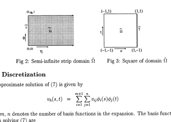
Fig 2: Semi-infinite strip domain $\tilde{\Omega}$

Fig 3: Square ofdomain $\hat{\Omega}$

$2.2$

Discretization

The approximate solution of (7) is given by

(8) $v_{h}(s, t)$ $= \sum_{i=1}^{m+}\sum_{1j=}^{n}v_{i}1j\phi_{i}(S)\phi_{j}(t)$

where $m,$ $n$ denotes the number of basis functionsin the expansion. The basisfunctions

used in solving (7)

are

$\phi_{k}(\mathit{8})$ $=$ $\frac{1}{\sqrt{4k+2}}(P_{k-1}(s)-P_{k1}+(s)),$ $k\neq m+1$ ,

$\phi_{m+1}(s)$ $=$ $\omega(s)=(s+1)^{3}(-\frac{3}{16}\mathit{8}+\frac{5}{16})$

where $P_{k}(\mathit{8})$ is the Legendre polynomial of degree $k(\mathrm{S}\mathrm{e}\mathrm{e}[3]15])$.

The boundarybasis functions$\omega(s)$ isnecessary to satisfy thenonhomogeneous

bound-ary conditions at theboundaries. This basisfunction

was

pickedforits smoothness

over

the $\hat{\Omega}$

and its behavior at the boundary $\hat{\gamma}$. Here the basis function $\omega(s)$ is chosen to

satisfy

(9) $\{$

$\omega(1)=1$ $\omega’(1)=0$

$\omega(-1)=\omega^{r}(-1)=\omega\prime\prime(-1)=0$

Now

we

consider the nonhomogeneous boundary condition

on

$\hat{\gamma}$. We arrange the

nodes of $\hat{\gamma}$ in

an

order according to the anticlockwise direction. Let the number of

nodes be $n$ and $\{t_{j}\}_{j=1}^{n}$ be the nodes

on

the boundary $\hat{\gamma}$. The nodal values

on

$\{t_{j}\}_{j}^{n}=1$

are

also arranged in

an

order, which

are

denoted by $\hat{b}_{1},\hat{b}_{2},$_$\cdots$,$\hat{b}_{n}$, and they form a

n-dimensional column vector $\hat{\mathrm{b}}=(\hat{b}_{1},\hat{b}_{2n}, \cdots,\hat{b})^{\tau}$, where by $T$

we

refer to the transpose

of

a

matrix

or a

vector.

We obtain from (7),(8)$,(9)$ that

(10)

’

$\hat{b}_{l}$

Let $\phi_{j}(t_{l})$ be the entries ofthe matrix $\mathrm{H},$ (10)

can

be written in the form

(11) $\mathrm{H}^{T}\mathrm{v}_{0}$ _$=$

$\hat{\mathrm{b}}$

where $\mathrm{v}_{0}=(v_{m+1,1}, ?)_{m+}1,2,$$\cdots,$$v_{m+}1,n)^{\tau}$. Therefore,

we

can

obtain $\{v_{m+1,j}\}_{j=1}^{n}$ by

solv-ing (11).

Orthogonalizing the residual against basis functions $\phi_{p}(\mathit{8})\phi_{q}(t)$ byusing

a

inner

prod-uct yields

(12) $\int_{\Omega}\phi_{p}\phi_{q}\frac{\partial}{\partial s}(\frac{1}{\psi_{s}}, \frac{\partial v_{h}}{\partial s})\psi’tSddt+\int_{\Omega}\phi_{p}\phi_{q}\frac{\partial}{\partial t}(\frac{1}{\psi_{t}}, \frac{\partial v_{h}}{\partial t})\psi_{S}’d_{S}dt$ $=$ $\int_{\Omega}\phi_{p}\phi_{q}\psi s\hat{f}\psi^{l}td\mathit{8}\prime dt$.

Substituting (8) into (12),

we

obtain

$\sum_{i=1}^{m+1}\sum^{n}j=1?)ij\int-1d_{\mathit{8}\int_{-1}d}1\phi p\frac{1}{\psi_{S}’}\phi\prime\prime i1\phi_{j}\psi t’\phi_{q}t$ $+$ $\sum_{i=1}^{m+}1j=\sum \mathrm{t}n1)ij\int_{-}1\phi_{p}\psi_{S}\phi_{i}d\mathit{8}\int_{-1}1d\prime 1\phi_{j^{\frac{1}{\psi_{t}’}\phi_{q}’}}’t$

(13) $=$ $\int_{\Omega}\phi_{p}\phi_{q}\psi’s\hat{f}\psi’\iota dd\mathit{8}t$.

Setting $\mathrm{V}=[v_{ij}],$ $1\leq i\leq m,$ $1\leq j\leq n,$ (13)

can

be written in the form

(14) $\mathrm{A}\mathrm{V}\mathrm{B}+\mathrm{C}\mathrm{V}\mathrm{D}$ $=\mathrm{F}$

where

A $=$ $\{a_{\dot{\mu}}\}_{p},i=1,2,\cdots,m$

,

$a_{pi}= \int_{-1}^{1}\phi_{p}^{l}\frac{1}{\psi_{s}’}\phi_{i}’d\mathit{8},$ $\mathrm{C}=\{c_{P}i\}_{p},i=1,2,\cdots,m$ , $c_{pi}= \int_{-1}^{1}\phi_{p}\psi’s\phi_{i}d_{\mathit{8}}$ ,

$\mathrm{B}$ _$=$ $\{b_{jq}\}_{j,2,\cdots,n}q=1,)b_{jq}=\int_{-1}^{1}\phi_{j}\psi t\phi_{q}dt$

’

, $\mathrm{D}=\{d_{jq}\}_{j,2,\cdots,n}q=1,$

,

$d_{jq}= \int_{-1}^{1}\phi_{j^{\frac{1}{\psi_{t}’}\phi d}}’qt’$.

The entries $f_{pq},$ $1\leq p\leq m,$$1\leq q\leq n$ of the matrix$\mathrm{F}$

are

given by

$f_{pq}$ $=$ $\int_{\Omega}\phi_{p}\emptyset_{q}\psi_{S}’\hat{f}\psi t-d\mathit{8}dt\sum^{n}\prime v_{m+1,j}bj=1jq\int_{-}1n)1\phi p\frac{1}{\psi_{S}’}\omega d\prime r\mathit{8}-\sum\iota j=1m+1,jdjq\int_{-}1\phi_{p}1\psi_{s}\omega d_{S}’$.

$a_{pi},$ $c_{/pi},$ $f_{pq}$ can be given by using Gauss-type quadrature rules. On the other hand,

using the orthogonality relation

$\int_{-1}^{1}P_{i}(t)P_{j(}t)dt$ $=$ $\frac{2}{2j+1}\delta_{ij}$

and the

recurrence

relation

$(2j+1)P_{j}(t)$ $=$ $P_{j+1}’(t)-P’-1(jt)$.

leads to

$b_{ji}=b_{ij}$ $=$ $\{$

$c_{i}c_{j}( \frac{\alpha}{2j-1}+\frac{\alpha}{2j+3})i=j$

$-C_{i}C_{j^{\frac{\alpha}{2i-1}}}$ $i=j+2$

$d_{ij}=$

where $c_{j}=1/\sqrt{4j+2}$.

Weconsider the following eigenvalue problem$(\alpha/2)\mathrm{B}\mathrm{x}=\lambda \mathrm{x}$andlet $\Lambda$be the diagonal

matrix formed the eigenvalues and let X be the matrix formed by the corresponding

eigenvectors. Then

(15) BX $=$ $\mathrm{D}\mathrm{X}\Lambda=\frac{2}{\alpha}$XA

Making

a

change of variable $\mathrm{V}=\mathrm{W}\mathrm{X}^{T}$ in (14),

we

find

(16) $\mathrm{A}\mathrm{W}\mathrm{X}^{T}\mathrm{B}+\mathrm{C}\mathrm{W}\mathrm{X}^{\tau}\mathrm{D}$ _$=$ F.

We then derive from (15) that

(17) $\mathrm{A}\mathrm{W}\Lambda+\mathrm{c}\mathrm{W}$ _$=$ $\mathrm{G}$

where $\mathrm{G}=(\alpha/2)\mathrm{F}\mathrm{X}$. Let $\mathrm{w}_{j}=(w_{1j}, w_{2}j, \cdots, wmj)^{T}$ and $\mathrm{g}_{j}=(g1j, g2j, \cdots, \mathit{9}mj)T$ for

$j=1,2,$ $\cdots n\}$. Then the$j\mathrm{t}\mathrm{h}$ column ofequation (17)

can

be written

as

(18) $(\lambda_{j}\mathrm{A}+\mathrm{c})\mathrm{W}_{j}$ $=$ $\mathrm{g}_{j}$.

In summary, the solution of (14) consists of the following step:

1. Compute the eigenvalues and eigenector $\mathrm{s}$ of

$\mathrm{B}$

2. Compute $\mathrm{G}$

3. Obtain$\mathrm{W}$ by solving (18)

4. Set $\mathrm{V}=\mathrm{W}\mathrm{X}^{T}$.

Since $\mathrm{B}$

can

besplit into two symmetric tridiagonal submatrices, the eigenvalues and

eigenvectors of$\mathrm{B}$

can

be easily computed in $O(n^{2})$. Steps 2,3,4 take $O(mn^{2}),$ $O(nm^{3})$,

$O(mn^{2})$, respectively. Therefore, the system (14)

can

be solved in about $O(mn^{2}+nm^{3})$.

3

Numerical Experiments

In thissection,

we

present

some

numerical experiments. All computations

are

performed

in double precistion

on

the Sun $\mathrm{U}\mathrm{l}\mathrm{t}\mathrm{r}\mathrm{a}\mathrm{s}\mathrm{p}\mathrm{A}\mathrm{R}\mathrm{c}2$ workstation.

Consider the problem on the fan-shaped domain $\Omega$ with a interior angle $\alpha$

$-\nabla^{2}u(_{X}, y)$ $=$ $f(x, y),$ $(x, y)\in\Omega$ ,

$u(x, y)$ $=$ $0$ , $(x, y)\in\partial\Omega$

where $f(x, y)$ is chosen

so

that the exact solution is given by

Fig 4: Solution for $\alpha=7\pi/4$

Let $u_{h}(x, y)$ be the approximate solution

on

the domain $\Omega$. We define the

Legendre-Galerkin error

norm

by

(19) $||E_{U}||$ $=$ _{$() \max_{x,y\in U}|u(x, y)-uh(_{X}, y)|$}

where

$U$ $=$ $\{(0.9^{k}\cos(j\alpha/50), 0.9^{k}\sin(j\alpha/50)):0\leq k\leq 50,0\leq j\leq 50\}$.

We set $\alpha=7\pi/4$ and _$m=an$. A mesh plot of the approximate solution is shown in

Fig 4. Comparing the numerical solutions with the exact solutions by (19),

we

obtain

the approximate error

norm as

shown in Fig 5.

Let usmake an analysis of the result $\mathrm{s}\mathrm{h}_{0\backslash }\mathrm{v}\mathrm{n}$ in Fig 5. From the result the approximate

error

normobserved to be declining with increasing the valuesof$a$, but if$a$is

more

than

5/2, the increasing of$a$ has

no

significantinfluence to the result. Then,

we

can

conclude

that the values of$n$ and $m$ should be adjusted to each other for reasonable accuracy. In

addition,

as

$\mathrm{s}\mathrm{h}_{0\backslash }\mathrm{v}\mathrm{n}$in Fig 6, when

$a$ is

more

than 5/2, the Legendre-Galerkin method

has the exponential

convergence

rate.

When setting $m=3n$ ,

we

can

obtain reasonable accuracy although the angle $\alpha$

becomes bigger

as

shown in Fig 6.

4

Conclusion

We proposed the Legendre-Galerkin method for solving Poisson’equation

on

a

fan-shaped domain. Our proposed method leads to high accuracy and in conjunction with

the domain decomposition method it

can

be applied to solve the problems with

rlg $0$:

vonvergence

rates wlrn $n$

rlg $\mathfrak{o}$:

vonvergence

rates wlrn $\alpha$

References

[1] F.Stenger. Numerical Methods Ba8ed on Sinc and Analytic Function8, volume 20

of Computational Mathematics. Springer-Verlag, 1993.

[2] $\ovalbox{\tt\small REJECT}\hslash,$ $\mathrm{p},\ovalbox{\tt\small REJECT}_{\backslash },$ 2

$\ovalbox{\tt\small REJECT} \mathrm{f}\mathrm{f}\mathrm{i}\mathfrak{F}\ovalbox{\tt\small REJECT}\Re\ovalbox{\tt\small REJECT}_{\mathrm{A}\mathrm{a}^{\ovalbox{\tt\small REJECT}}\Phi}^{\ovalbox{\tt\small REJECT}}\mathrm{x}\xi \mathrm{f}\mathrm{f}\mathrm{l}’)r.arrow$Sinc-Galerkin

g,

$\mathrm{B}*r\llcorner\backslash \mathrm{f}\mathrm{f}\mathrm{l}\mathrm{a}\Phi \mathrm{F}$

$\infty\ulcorner’=^{\overline{\backslash _{\underline{\backslash }}}}\ulcorner\Re 8\not\in_{\mathrm{x}}\mathrm{P}\not\in_{\mathrm{r}\mathfrak{F}^{\backslash }}^{\infty}\mathrm{g}\#\ovalbox{\tt\small REJECT}\ovalbox{\tt\small REJECT}$ , 1996,

p142-143

[3] J. Shen,Efficient Spectral-Galerking 1. Direct solvers

_for

second- and

_fourth-order

equation by using Legendre$polynomail\mathit{8}_{i}$ SIAM J.Sci. Comput., 15(1994), pp.

[4] Nancy J. Lybeck, Kenneth L.Bowers, Sinc Methods

_for

Domain $DecomP^{O}\mathit{8}iii_{\mathit{0}}n$,

Applied Mathematics and Computation, Vol. 75, 13-41(1996)

[5] Nancy J. Lybeck, Kenneth L.Bowers, Domain Decompo8ition in Conjuction with

Sinc Methods

_for

Poisson’s Equation, Numerical Methods for Partial Differential

Equation, Vol. 12, 461-486(1996)

[6] ナラーティップ, 杉浦, 三角形領域における Poisson方程式に対する Sinc-Galerkin

Schwarz Alternating法について, 第28回数値解析シンポジウム講演予稿集

_P92-95