Pattern dynamics of a reaction-diffusion-advection system with bistable growth (Qualitative theory of ordinary differential equations in real domains and its applications)

Pattern dynamics of

a

reaction-diffusion-advection

system

with

bistable

growth

*

Tohru

Tsujikawa\dagger

Faculty of Engineering, University

of

Miyazaki

Miyazaki

889-2192

1

Introduction

From

a

viewpoint of the pattern formation in Biology, reaction diffusion systems are

treated. In this paper we consider the following chemotaxis-growth model $(e.$ $g.$ $[2],$ $[8],$

[20]).

$\{\begin{array}{ll}u_{t}=\mathcal{D}\{u_{x}-\alpha uv_{x}\}_{x}+f(u) , in I\cross \mathbb{R}_{+},v_{t}=dv_{xx}+u-v, in I\cross \mathbb{R}_{+},u_{x}(x, t)=0, v_{x}(x, t)=0, on \partial I\cross \mathbb{R}_{+},u(\cdot, O)=u_{0}\geq 0, v(\cdot, 0)=v_{0}\geq 0, in I\end{array}$ (1)

where $\mathcal{D},$ $d$, a are positive constants and $I=(O, 1)$. In the absence of growth term $f(u)$,

this system becomes Keller-Segel type and many people study about steady states, blow

up etc.. On the other hand, for (1) it is known several spatio-temporal patterns due to the

Turing and Hopf instability induced by the chemotaxis effect $(e. g. [7], [12], [3])$. In order

to understand mechanism of these pattern formations, we show the existence of global

solutions and an exponential attractor with finite dimension of (1) $(e.$ _$g$. [1], [9], [11],

[17]) Moreover, the existence and stability of stationary solutions of (1) is discussed

for several growth terms [4, 5, 6, 7]. By using Degree theory, bifurcation method and

etc., the existence of the stationary solution is locally shown with $respec^{l}t$ to parameters

$\mathcal{D},$ $d,$$\alpha(e. g. [17], [19], [5])$. But it is difficult to show the global structure ofstationary

solutions with respect to parameters. In this paper, we treat the bistable growth term

$f(u)=u(1-u)(u-a)(0<a<1)$

and study the global structure ofstationarysolutions

of (1)

as

large $\mathcal{D}$. To do so, we

assume

that $(u, v)$ is uniformly

bounded

as

$\mathcal{D}$

tends to

$\infty$. Formally, it holds that $\{u_{x}-\alpha uv_{x}\}_{x}=0$

.

It follows from the boundary conditions of

$*$

This is a joint work with Hirofumi Izuhara (University of Miyazaki) and Kousuke Kuto (The UniversityofElectro-Communicatons)

$\uparrow e$

$u,$ $v$ that $u$ is represented by $u=Ee^{\alpha v}$ with any positiveconstant $E$. By integrating the

first equation of (1) on $I$, (1) deduces to the following system:

$\{\begin{array}{ll}(\int_{0}^{1}Ee^{\alpha v}dx)_{t}=\int_{0}^{1}f(Ee^{\alpha v})dx, t>0v_{t}=dv_{xx}+g(v, E) , x\in I, t>0v_{x}(0, t)=v_{x}(1, t)=0, t>0u\geq 0, v\geq 0, x\in I, t>0,\end{array}$ (2)

where $g(v, E)=Ee^{\alpha v}-v$_{. Here}

_we

_{call (2) a shadow system of (1). We remark that}

_a

stationary solution of (1) converges to the corresponding solution of (2) infollowing

sense.

Remark 1.1. [18] Let $\{\mathcal{D}_{n}\}$ and $(u_{n}, v_{n})$ be a positive sequence with $\lim_{narrow\infty}\mathcal{D}_{n}=\infty$

and a stationary solution

_of

(1) with $\mathcal{D}=\mathcal{D}_{n}$. Then there exists a subsequence $\{\mathcal{D}_{n’}\}$

of

$\{\mathcal{D}_{n}\}$ and

a

stationary solution $(u_{\infty}, v_{\infty})$

of

(2) such that

$\lim_{narrow\infty}(u_{n’}, v_{n’})=(u_{\infty}, v_{\infty})$ $in$ $C^{1}(\overline{\Omega})\cross C^{1}(\overline{\Omega})$. (3)

Therefore, it is important to treat (2) for understanding stationary solutions of (1) for

large $\mathcal{D}$.

But

we

havenot any similar result with respect to the evolution problem of (1),

In this paper

we

consider the stationary problem of (2)

as

follows:

$\{\begin{array}{ll}dv_{xx}+9(v, E)=0, x\in I,u_{x}(x)=v_{x}(x)=0, x\in\partial Iu\geq 0, v\geq 0, x\in I\end{array}$ (4)

and

$\int_{\Omega}f(Ee^{\alpha v})dx=0$. (5)

The organization of this paper is as follows: In Section 2, we summarize known results

of the existence of solutions of (4) and ourmain results for the stability of theses solution

is given in Section

3.

In Section 4, we demonstrate the global structure of stationary

solutions and periodic solution of (2). Finally, introducing a

new

small parameter, we

show the onset of the periodic solution is

an

infinite-dimensional

relaxation oscillation

which is governed by slow and fast dynamics.

2

Existence

of

the stationary solution

of

Shadow

Sy-stem

We summarize known results of the existence of solutions with respect to (4), (5).

Here-after wedescribe a solution of (4), (5) by $(v(x, d, E), d, E)$. All solution is represented

by the scaling, repetition and reflection of monotone solutions. Then we only consider

monotone increasing solutions.

First,

we

treat the boundary value problem (4) without the integral constraint (5).

Lemma 1. [6] There exists a positive constant

\^E.

Then, (4) has two positive constant

solution $v_{*}(E)$, $v^{*}(E)$

for

any $0<E<\hat{E}$ which satisfy $v_{*}(E)<v^{*}(E)$, $v_{*}(\hat{E})=v^{*}(\hat{E})$

and

are

monotone increasing and decreasing

_{function of}

$E$, respectively.

By using Lemma 1 and the bifurcation theory $(e. g. [13], [14], [15])$, we have

Lemma 2. For any$0<E<\hat{E}$, there exists a monotone decreasing

_function

$d^{*}(E)$ which

satisfies

$\lim_{Earrow 0}d^{*}(E)=\infty,$ $\lim_{Earrow\hat{E}}d^{*}(E)=0$. Then there is a solution $v(x, d, E)$

of

(4)

_for

any $0<E<\hat{E},$ _{$0<d<d^{*}(E)$ and it holds}

$\lim_{darrow d^{r}(E)}v(x, d, E)=v^{*}(E)$, $\lim_{darrow 0}v(x, d, E)=v^{B}(x, E)=\{\begin{array}{l}v_{*}(E) 0\leq x<1(6)\overline{v}(E) x=1\end{array}$

where $\overline{v}(E)$ is a constant satisfying $\int_{v_{*}(E)}^{\overline{v}(E)}g(v, E)dv=0.$

Thanks to the result of Schaaf [13], we show

Lemma 3. Let$\Lambda$ $:=\{(d, E)|0<E<\hat{E}, 0<d<d^{*}(E)\}$

. There is not any nonconstant

solution

_of

(4)

_for

$(d, E)\in \mathbb{R}_{+}^{2}\backslash \Lambda.$

Next, we obtain the existence of solutions of (4) whichsatisfies the integral constraint.

Let $h(d, E)$ _be

a

_{function of} $d$ and $E$ defined by

$h(d, E):= \int_{0}^{1}f(Ee^{\alpha v(x,d,E)})dx$ ₍₇₎

where $v(x, d, E)$ is

a

solution given in Lemma 2. Therefore, the integral constraint (5)

is represented by

$h(d, E)=0$. (8)

Then it holds that

Lemma 4. Let $\Lambda^{-}:=\{(d, E)|0\leq d\leq d^{*}(E), 0<E\leq\hat{E}\}$ _and$\Lambda^{0}$

$:=\{(d, E)|0<d\leq$

$d^{*}(E)$,$0<E\leq\hat{E}\}$

.

Then, $h(d, E)$

satisfies

$h(d, E)\in C(\Lambda^{-})\cap C^{1}(\Lambda^{0})$ and

$\lim_{darrow 0}h(d, E)=f(Ee^{\alpha v_{*}(E)})$. (9)

Setting

$\Gamma$

$:=$

{

$(v(x, d, E),$ $d,$ $E)|v(x, d, E)$ is asolution of (4), (5) for any $(d, E)\in\Lambda$

}

we can show the existence of stationary solutions

as

follows:

Theorem 5. [6] There are two positive constants $E_{a},$ $E_{1}$ $<\hat{E}$ depending

on

$a$, 1 and

following three statements hold

(i)

_If

$1/\alpha<a$_{, 1,} $E_{a},$ $E_{1}$ satisfy_{$E_{1}<E_{a}$} and there exists a

function

$d(E)$

defined

on

the interval $(E_{1}, E_{a})$ and $(v^{\epsilon}(x, d(E), E), d(E), E)\in\Gamma$

.

Moreover,

(ii)

_If

$a<1/\alpha<1$, there exists

a

_function

$d(E)$

defined

on

$(E_{1}, E_{a})$ or $(E_{a}, E_{1})$ and

$(v^{s}(x, d(E), E), d(E), E)\in\Gamma$, which

_satisfies

$\lim_{Earrow E_{1}}v^{s}(x, d(E), E)=v^{*}(E_{1}) , \lim_{Earrow E_{a}}v^{s}(x, d(E), E)=v^{B}(x, E_{a})$. (11)

(iii)

_If

$1/\alpha>a$_{, 1,} then $E_{a},$ $E_{1}$ satisfy _{$E_{a}<E_{1}$} and there exists

a

function

$d(E)$

defined

on

$(E_{a}, E_{1})$ and _{$(v^{s}(x, d(E), E), d(E), E)\in\Gamma$,} which

satisfies

$\lim_{Earrow E_{1}}v^{s}(x, d(E), E)=v^{B}(x, E_{1}) , \lim_{Earrow E_{a}}v^{s}(x, d(E), E)=v^{B}(x, E_{a})$. (12)

We call $v^{B}(x, E)$

a

_{singular solution with} a _{boundary layer. In the next section, we}

discuss the stability ofthese singular solutions.

3

Stability

of stationary solution of Shadow System

In this section we show the stability of stationary solutions of (2), which are given in

Theorem

5.

First

we

discuss astabilityofthe singular stationary solution witha boundary

layer obtained inTheorem 5

as

$d$is small. Let _{$(v^{s}(x, d, E), d, E)$} be

a

solution of

(4), (5) for

$(d, E)\in\Lambda$ in the neighborhood of $(0, E_{a})$, which satisfies $\lim_{d\downarrow 0}v^{s}(x, d, E)=v^{B}(x, E_{a})$.

In order to study a stability, we consider the following linearized eigenvalue problem

around the solution $(v^{s}(x, d, E), d, E)$ of (2):

$\{\begin{array}{l}\lambda\int_{0}^{1}(\eta+E\alpha w)e^{\alpha v^{S}}dx=\int_{0}^{1}f_{u}(Ee^{\alpha v^{S}})(\eta+E\alpha w)e^{\alpha v^{s}}dx\lambda w=dw_{xx}+9v(v^{S}, E)w+g_{E}(v^{s}, E)\eta, x\in(0,1)w_{x}(0)=w_{x}(1)=0,\end{array}$

(13)

where $g_{v}(v, E)=E\alpha e^{\alpha v}-\gamma,$ _{$9E(v, E)=e^{\alpha v}$. Here, $(\eta, w(x))$ means an eigenfunction}

of the eigenvalue $\lambda$

and $\eta$ is a positive constant.

As $darrow 0$_, we _{show the asymptotic behavior of critical eigenvalue which determines}

the stability by using the SLEP method (see [10]).

Theorem 6. [6] Set $1/\alpha>a$_. Let $(v^{s}(x, d, E), d, E)$ be a _stationary solution

of

₍₂₎

_for

$(d, E)\in$ A _{in the neighborhood}

_of

$(0, E_{a})$, which

satisfies

$\lim_{d\downarrow 0}v^{s}(x, d, E)=v^{B}(E_{a})$

.

Then, there

are

two eigenvalues $\lambda_{1}(d)$, $\lambda_{2}(d)$ with positive real part such that

$\lim_{darrow 0}\lambda_{1}(d)=f_{u}(a)>0,$ $\lim_{darrow 0}\lambda_{2}(d)=\theta^{*}>0$ (

$\theta^{*}$

is given in Lemma 7).

Moreover, other eigenvalues have negative real part and uniformly away

_from

imaginary axis.

We discuss about this result by intuition. If $w(x)$ has _not any singularity in the

neighborhood of $x=1$, we have formally $\lim_{darrow 0}\lambda=f_{u}(a)$ because of

$\lim_{darrow 0}f_{u}(Ee^{\alpha v^{s}})=f_{u}(a)$ compact uniformly in $[0$,1)

On the other hand, if $w(x)$ has

a

singularity in the

neighborhood

of $x=1$, then $\eta=$

$0$ becomes

an

approximate eigenfunction. Therefore,

we

treat the following linearized

eigenvalue problem corresponding to (4), (5) around $v^{s}(x, d, E)$:

$\{\begin{array}{l}\lambda w=dw_{xx}+g_{v}(v^{s}, E)w, x\in(0,1) ,(14)w_{x}(0)=w_{x}(1)=0.\end{array}$

Then, we show the following Lemma.

Lemma 7. There is only

one

eigenvalue $\hat{\lambda}(d)$ with positive real part

of

the linearized

eigenvalue problem (14), which

_satisfies

$\lim_{darrow 0}\hat{\lambda}(d)=\theta^{*}>0.$

By using

a

similar argument,

we

have

Theorem 8. [6]

Set

$1/\alpha>1$. Let $(v^{s}(x, d, E), d, E)$ be a stationary solution

of

(2)

for

$(d, E)\in\Lambda$ in the neighborhood

of

$(0, E_{1})$, which

satisfies

$\lim_{d\downarrow 0}v^{s}(x, d, E)=v^{B}(x, E_{1})$

.

Then, there is only

one

eigenvalue $\lambda^{*}(d)$ with positive realpart such that

$\lim_{darrow 0}\lambda^{*}(d)=\theta^{*}>0.$

Moreover, other eigenvalues have negative real part and uniformly away

_from

imaginary

axis. Here $\theta^{*}$ is a constant depending

on

_{$E=E_{1}$}

given in Lemma

7.

Next,

we

showthe stability ofthe nonconstant bifurcatingsolutions from the constant

solution in the neighborhood of the bifurcation point.

Theorem 9. [6]

_If

$1/\alpha<a$, 1, the following statements hold.

(1) Let $(v^{s}(x, d, E), d, E)$ be a solution

of

(2)

for

$(d, E)\in\Lambda$ in the neighborhood

of

$(d^{*}(E_{a}), E_{a})$, which

satisfies

$\lim_{darrow d^{r}(E_{a})}v^{s}(x, d, E)=v^{*}(E_{a})$

.

Then, there exists

only

one

eigenvalue $\lambda^{*}(d)$ with positive realpart such that

$\lim_{darrow 0}\lambda^{*}(d)=f_{u}(a)>0.$

Moreover, other eigenvalues have negative real part and uniformly away

_from

ima-ginary axis.

(2) Let $(\tau)^{s}(x, d, E)$,$d,$ $E$) be a solution

of

(2)

for

$(d, E)\in\Lambda$ in the neighborhood

of

$(d^{*}(E_{1}), E_{1})$_, which

satisfies

$\lim_{darrow d^{*}(E_{1})}v^{s}(x, d, E)=v^{*}(E_{1})$. Then, all eigenvalues

have negative real part and uniformly away

_from

imaginary axis.

4

Numerical results

In this section, we discuss the existence and stability of stationary solutions of (2) by

the numerical approach. When $\alpha=2.0$ _{and $a=0.25$, that is, the}

case

_{(ii) of}

The-orem 5, there is a singular solution $v(x, d(E), E)$ with a boundary layer, which satisfies

which satisfies $\lim_{Earrow E_{1}}(v^{s}(x, d(E), E), d(E))=(v^{*}(E_{1}), d^{*}(E_{1}))$. We show the global

bi-furcation

branch connecting these two solutions $v^{B}(x, E_{a})$ and $v^{*}(E_{1})$ in Figure 1 (a),

which is numerically

obtained

by the

AUTO

package [1]. Here each point $(d, E)$ on the

curve

of this figure (a) corresponds to a monotone increasing solution of (4), (5). From

this result, there is not (static) secondary bifurcation phenomena from nonconstant

so-lution on the bifurcation branch. But, the solution is unstable for small $d$, that is, there

are two eigenvalues with a positive real part from Theorem

9.

On the other hand, the

solutions for $(d, E)$ _{in the neighborhood of} $(d^{*}(E_{1}), E_{1})$

are

stable from Theorem

9

(2).

The number ofeigenvalues with respect to stationary solutions

on

the bifurcation

curve

changes depending

on

the parameter $d.$

(a) (b)

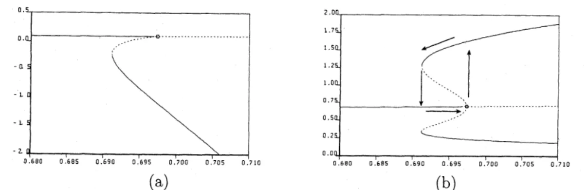
Figure 1: The global solution structure for $\alpha=2.0$, where the symbol ◇

means a

bifur-cation point. (a) Vertical and horizontal axis mean parameters $d$and $E$, respectively. (b)

Vertical and horizontal axis mean the value of $v$ at $x=1$ and $d$, respectively.

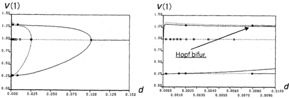
For the original reaction diffusion system (1), the global bifurcation from the constant

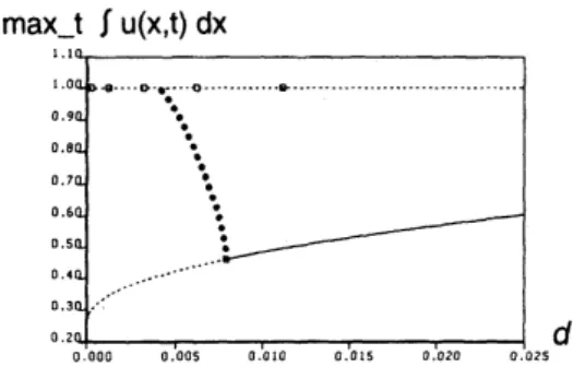
solution is obtained by the numerical simulation (see Figure 2). From Figure 2 implies the existence ofthe Hopfbifurcation from the nonconstant solution in the neighborhood at $d=0.008$. Moreover, these periodic solutions are stable from Figure 3. Therefore, we

suggestthat there is a Hopfbifurcation phenomenafor the shadowsystem (2). Therefore,

we guess the change of the number ofeigenvalues with a positive real part.

$y(1)$

Figure 2: Vertical and horizontal axises

mean

the maximal value of $v(x)(v(1))$ and $d.$

$\max_{-}t$

;

$u(x,t)dx$

Figure 3: Vertical and horizontal axises

mean a

maximal value of $\Vert u(\cdot, t)\Vert_{L^{1}}$ and $d.$

$\mathcal{D}=100.,$ $\alpha=2.0,$ $a=0.25.$

5

Relaxation

oscillation

In Section 4,

we

show that the periodic solution of (1) exists due to the secondary bi-furcation phenomena from the monotone solution

as

large $\mathcal{D}$

and is stable by numerical

computations (see Figures $2-3$). It is difficult to show the Hopf bifurcation from the

nonconstant solution for

our

limiting system (2). But

we

suggest the appearance of the

periodic pattern from the lose of stability in Section 3. Therefore,

we

discuss about the

appearance ofthis phenomena from the other viewpoint. To do so,

we

demonstrate the

infinite dimensional relaxation oscillation

as

the onset of these spatio-temporal

pheno-mena

(see [3, 4 In order to explain that,

we

introduce

a

new

parameter$\delta$

which

mean

the rate ofthe growth. Then, we have the following system with respect to (2):

$\{\begin{array}{ll}(\int_{0}^{1}Ee^{\alpha v}dx)_{t}=\delta\int_{0}^{1}f(Ee^{\alpha v})dx, t>0v_{t}=dv_{xx}+g(v, E) , x\in(0,1) , t>0v_{x}(0, t)=v_{x}(1, t)=0, t>0\end{array}$ (15)

where $E(t)$_, $v(x, t)$

are

unknown functions.

Figure 4 implies the existence of periodic solution of (15) for small $\delta$

by a numerical

simulation.

Figure 4: Periodic pattern with respect to $v(x, t)$ of (15) for _$d=0.04,$ $\alpha=2.0,$ $\delta=$

According

to the argument in [3, 4],

we

show that the behavior of the solution is described by the fast and slow dynamics derived from (15) as $\delta$ is sufficiently

small.

Fast dynamics

First, we consider the

case

of $\delta=0$

as

follows:

$\{\begin{array}{l}(\int_{0}^{1}Ee^{\alpha v}dx)_{t}=0, t>0v_{t}=dv_{xx}+g(v, E) , x\in(0,1) , t>0v_{x}(0, t)=v_{x}(1, t)=0, t>0.\end{array}$

(16)

It follows from the first equation of (16) that

$\int_{0}^{1}Ee^{\alpha v}dx=\mu$ ₍₁₇₎

for any positive constant $\mu.$

We already discuss the constant solution of (16) in Lemma 1.

On

the other hand, the

stationary solution $v(x)$ satisfies

$\int_{0}^{1}Ee^{\alpha v}dx=\int_{0}^{1}vdx (=\mu)$ ₍₁₈₎

by integrating the first equation of(4) and using the boundary condition of$v$. Therefore,

a

constant solution $(E_{c}, v_{c})$ is represented by $E_{c}=\mu e^{-\alpha\mu},$

$v_{c}=\mu$ for any $\mu>0.$

In order to have nonconstant solutions by using the bifurcation method, we consider

the linearized eigenvalue problem around $(E_{c}, v_{c})$. By setting $E=E_{c}+Mv=\mu+V$ and

substituting this into (16), the linearized eigenvalue problem is written by

$\{\begin{array}{ll}M_{t}=-E_{c}\alpha\{Me^{\alpha\mu}+(\alpha\mu-1)\int_{0}^{1}Vdx\}, t>0V_{t}=dV_{xx}+Me^{\alpha V}+(\alpha\mu-1)V, x\in(0,1) , t>0V_{x}(0, t)=V_{x}(1, t)=0, t>0.\end{array}$

(19)

Substituting $M=\phi e^{\lambda t},$ $V=\psi e^{\lambda t}\cos n\pi x$ into (19), we _{have $\phi(\lambda+\alpha\mu)=0,$} $\psi(\lambda+$

$d(n\pi)^{2}-\alpha\mu-1)=$ _{O. When} $\lambda=0$_, it holds that _{$\phi=0,$ $\alpha\mu=d(n\pi)^{2}-1$. Because}

of $d>0$, we get the condition $\alpha\mu-1>$ O. There are two constant _{solutions of (4) in}

Lemma 1. Then, $v^{*}(E)$ satisfies this condition. The curve in Figure 5 _{(a) corresponds to}

$\lambda=0$ in

$\mu-\alpha$ plane, which is the mode $n$ perturbations. On the other hand,

we

show

the nonconstant _{solution subcritically bifurcating from the constant solution} $v^{*}(E)$ and

subsequentlyturnthe direction due to saddle-node bifurcation in Figure5 (b). Therefore,

there appears ahysteresis phenomena. That is, thebifurcating solutionfromthe constant

solution becomes unstableand

recovers

the stability after the saddle-node bifurcation. We

remark that the direction ofbifurcating branch is different depending on $\alpha.$

Therefore, anapproximation $(E_{c}(\mu), v_{c}(x, \mu, d))$ of stationarysolutions of_{(15) satisfies}

(a) (b)

Figure 5:

$f(u)=u(1-u)(u-O.25)$

, $d=0.04$, (a) Vertical and horizontal axises

mean

$\alpha$ and $\mu$, (b) Vertical and horizontal axises

mean

$v(O)$ and $\mu,$ $\alpha=2.0$. There is a first

bifurcation at $\mu=0.697$ and

saddle-node

at $\mu=0.697.$

Slow dynamics

Next,

we

assume

that the solution of(15) tends to

some

monotone stationary solution

on

the upper branch in Figure

5

(b). Then, the solution is governed by the dynamics

with the slow time scale $T=\delta t$. Therefore, by using the

new

time variable $T$ andsetting

$\delta=0$, (15) is rewritten

as

$\{\begin{array}{ll}(\int_{0}^{1}Ee^{\alpha v}dx)_{T}=\int_{0}^{1}f(Ee^{\alpha v})dx, T>00=dv_{xx}+g(v, E) , x\in(0,1) , T>0v_{x}(0, T)=v_{x}(1, T)=0, T>0.\end{array}$ (21)

Since the relation (17) from (16) is shown, $\mu(t)$ satisfies

$\frac{d\mu}{dT}=\int_{0}^{1}f(Ee^{\alpha v})dx$ (22)

for

a

solution $(E_{s}(\mu),$ $v^{s}(X, \{\iota, d))$ of (21). Therefore, the behavior of the solution is

expressed by (22).

Figure 6 (a) shows that $\int_{0}^{1}f(E(\mu)e^{\alpha v_{c}})dx=f(E(\mu)e^{\alpha v_{c}})$ is positive on the constant

solution brunch corresponding to the center line in Figure6 (b). Therefor, $v_{c}$ is increasing

with respect to $T$. But the solution is destabilized as it passes the bifurcation point and

eventually tends to the stable

nonconstant

solution.

On

the other hand, the value of

integration $\int_{0}^{1}f(E(\mu)e^{\alpha v_{s}^{+}})dx$ is negative

on

the upper branch in Figure 6 (b).

There-fore, the solution $\mu(t)$ is decreasing with respect to $T$ and tends to the constant solution

through the saddle-node bifurcation point. Thereafter these process is periodically

repe-ated. Therefore the appearance of the relaxation oscillation phenomena is heuristically

(a) (b)

Figure 6:

$f(u)=u(1-u)(u-O.25)$

, $d=0.04,$$\alpha=2.0(a)$ Vertical and horizontal axises

mean

$v(O)$ and $\mu$, (b) Vertical and horizontal axises

mean

$\int_{0}^{1}f(Ee^{\alpha v})dx$ and

$\mu.$

References

[1] M. Aida, T. Tsujikawa, M. Effendiev, A. yagi and M. Mimura, Lower estimate of

at-tractor dimension for chemotaxis growth system, Journal

_of

the London Mathematical Society, 74 (2006),

453-474.

[2] W. Alt and D. A. Lauffenburger, Transient behavior ofa chemotaxis system modeling

certain types oftissue inflammation, J. Math. Biol., 24 (1987), 691-722.

[3] S.-I. Ei, H. Izuhara and M. Mimura, Infinite dimensional relaxation in

aggregation-growth systems, Discrete

Contin.

Dyn. Syst. Ser. B,

17

(2012),

1859-1887.

[4] S.-I. Ei, H. Izuhara and M. Mimura, Spatio-temporal oscillations irl the Keller-Segel

system with logistic growth, Physica D,

277

(2014), 1-21.

[5] C. Gai, Q. Wangand J. Yan, Qualitative analysis of stationaryKeller-Segel chemotaxis

models with logistic growth, preprint.

[6] H. Izuhara, K. Kuto and T. Tsujikawa, Bifurcation structure of stationary solutions

for a chemotaxissystem with bistable growth, preprint.

[7] K. Kuto, K. Osaki, T. Sakurai, T. Tsujikawa, Spatialpattern ina

chemotaxis-diffusion-growth model, Physica D, 241 (2012),

1629-1639.

[8] M.

Mimura

and T. Tsujikawa, Aggregating pattern dynamics in

a

chemotaxis model

including growth, Physica A, 230 (1996),

499-543.

[9] E. Nakaguchi and K. Osaki, Globalsolutions andexponentialattractorsofa

parabolic-parabolic systemfor chemotaxis with subquadratic degradation, Discrete Contin. Dyn.

Syst. Ser. B, 18 (2013),

2627-2646.

[10] Y. Nishiura and H. Fujii, Stability of singularly perturbed solutions to systems of

[11] K. Osaki, T. Tsujikawa,

A.

Yagi and M. Mimura, Exponential attractor for

a

chemotaxis-growth system of equations, Nonlinear Analysis $TMA.$ $51$ (2002),

119-144.

[12] K. J. Painter and T. Hillen, Spatio-temporal chaos in

a

chemotaxis model, Physica D, 240 (2011),

363-375.

[13] R., Schaaf,

Global

solution branches of two-point boundary value problems, Lecture

Notes in Mathematics, 1458, Springer-Verlag, Berlin,

1990.

[14] J. Shi, Semilinear Newmann boundary value problems

on

a rectangle,

7rans.

AMS,

354 (2002), 3117-3154.

[15]

J. Smaller

and

A.

Wasserman,

Global

bifurcation of steady-state solutions, J.

Diffe-rential Equations,

39

(1981),

269-290.

[16] I. Takagi, Point-condensation for.areaction-diffusion system, J.

_{Differential}

Equati-ons, 61 (1986),

208-249.

[17] J.I. Tello and M. Winkler, A chemotaxis system with logistic source, Comm. Partial

Differential

Equations, 35 (2007),

849-877.

[18] T. Tsujikawa, Stationary problem of

a

simple chemotaxis-growth model, RIMS

Kokyuroku, 1924 (2014),

55-63.

[19] T. Tsujikawa, K. Kuto, Y. Miyamoto and H. Izuhara, Stationary solutions for

some

shadow system of the Keller-Segel model with logistic source, to appear in DCDS-S,

2014.

[20] D. E. Woodward, R. Tyson, M. R. Myerscough, J. B. Murray, E.

O.

Budrene, B.

O.

Berg, Spatio-temporal patterns generated by Salmonella typhimurium, Biophys., 68