INTRODUCTION TO NON-DEGENERATE MIXED FUNCTIONS (Geometry on Real Closed Field and its Application to Singularity Theory)

INTRODUCTION TO NON-DEGENERATE MIXED FUNCTIONS

MUTSUO OKA

1. COMPLEX ANAYTIC HYPERSURFACE SINGULARITIES

Contents

Chaptcr 1. Complex analytic hypersurafcc singularities 1.1 Milnor fibration

1.2 Weighted homogeneous polynomial Chapter 2. Mixed function

2.1 Weighted homogeneous polynomlal

2.2 Mixed non-singularpoint

2.3

Transversality

2.4 Two special

cases

2.5 General mixed functions 2.6 Milnor flbration

Chapter 3. Mixed projective

curves

3.1 Canonical orientation

3.2 Milnor fibration and Hopf fibration

3.3 Degreeof mixed projective hypersurfacc

3.4 Twistedjoin typepolynomial

1.1. Milnor fibration. We first recallthe theoryofMilnor fibrations for

holomor-phic functions.

Let $f(z)$ be

a

holomorphic function of n-variables $z_{1},$$\ldots,$$z_{n}$ suchthat $f(0)=0$

.

As is well-known, J. Milnor proved that

Theorem 1. ([15])There exists a positive number$\epsilon_{0}$ such that the argument

map-ping

$\varphi:=f/|f|:S_{\epsilon}^{2r\iota-1}\backslash K_{\epsilon}arrow S^{1}$

is alocally trivial

_{fibration for}

any positive$\epsilon$ with$\epsilon\leq\epsilon_{0}$ where$K_{\overline{c}}=f^{-1}(0)\cap S_{e}^{2n-1}$

.

We call this the first description of Milnor fibration. Topologically $S_{\epsilon}\backslash$

$K_{\epsilon}\cong F\cross I/h$ : $Farrow F$

.

The characteristic polynomial is defined by $P_{n-1}(t)=$

$\det(h$

.

$-t id)$, where $h_{*}$ : $H_{n-1}(F)arrow H_{l-1}(F)$. $h_{*}$ is called monodromy

homomor-phism.

Theorem 2. ([15]) Suppose that $\epsilon$ is $s\uparrow,fficientl\uparrow/small$

as

in the above theorem.

Then $K$ is $(n-3)-$ connected. Suppose

further

that $O$ is an isolated singularity.

Then $F$has the homotopy type

of

a bouquet

of

spheres

of

$S^{n-1}$

Define

Euclidean inncr product and hermitian inner product:

$z=(z_{1}, \ldots, z_{n})=x+iy_{)}w=(w_{1}\ldots., w_{n})=u+iv$

$(z, w)=z_{1}\overline{w}_{1}+\cdots+z_{\iota}\overline{w}_{\iota}$, $(z, w)_{\mathbb{R}}=(x, u)+(y, v)=\Re(z, w)$

$\mathbb{C}^{n}\Leftrightarrow \mathbb{R}^{2n}$,

$z\Leftrightarrow(x, y)$

$f(z)=g(x, y)+ih(x, y)$

$gradg=(\frac{\partial g}{\partial x_{1}}, \ldots, \frac{\partial g}{\partial x_{n}}, \frac{\partial g}{\phi_{1}}, \ldots, \frac{\partial g}{\partial y_{n}})$

Tangent spaces:

$T_{Z}S_{\epsilon}=\{w\in \mathbb{C}^{r\iota}|\Re(z, w)=0\}$

$T_{Z}f^{-I}(t)=\{w\in \mathbb{C}^{n}|(w, gradf(z))=0\}$

$= \{w\in \mathbb{C}^{n}|w_{1}\frac{\partial f}{\partial z_{1}}+\cdots+\prime u)_{n}\frac{\partial f}{\partial z_{n}}=0\}$

$=\{w\in \mathbb{R}^{2n}| (w, gradg(z))_{\mathbb{R}}=(w, gradh(z))_{R}=0\}$

$T_{Z}F=\{w\in \mathbb{C}^{n}|\Re(w, z)=\Re(w, igrad\log(f(z))) =0\},$ $F=\varphi^{-1}(1)$

Note that

$\log f(z)=\log|f(z)|+i\arg(f(z))$, $f(z)/|f(z)|=\exp(i\arg(f(z))$.

Lemma 3. ([15]) $\varphi=f/|f|$ : $S_{\epsilon}arrow S^{1}$ is asubmersion

if

andonly

if

$\{z$, igrad$\log f(z)\}$

are linearly independent overR.

1.1.1. Cone theorem and the second

_fibmtion.

Suppose that $V=f^{-1}(0)$ has

an

isolated singularity at the origin. Then there exists a positive $\epsilon>0$ such that

$S_{r}rhV$ for any $0<r\leq\epsilon$. Note that $S_{r}rhV\Leftrightarrow T_{Z}S_{r}\supset T_{Z}V$

$\Leftrightarrow\forall z\in S_{r}\cap V,$

{

$z$, grad f(z)}: linearly independent over$\mathbb{C}$

Theorem 4. ([15]) Assume $O$ is an isolated singularity

of

V. Then there exists

a positive number $r_{0}>0$ so that

for

any $r,$ $0<r\leq r_{0},$ $S_{r}$

rn

V. In particular,

$(B_{r}, B_{r}\cap V)\cong$Cone$(S_{r}, K_{r})$

.

Wecall such $r_{0}$ a stable radius.

Proof.

Suppose there does not exists such $r_{0}$. By Curvc Selection lemma, one can

find

a

real analytic path

$p$ : $[0, \epsilon]arrow V,$ $p(t)\in V\backslash \{O\},$ $t\neq 0$ such that $p(t)$ is tangent to $V$. Thus we canwrite

$p(t)=\lambda(t)gradf(p(t)),$$t>0$.

Then

we

have

a

contradiction

as

follows. Put $\varphi(z)=(z, z)=\Vert z\Vert^{2}$ and $\phi=\sqrt{\varphi}$

.

$\frac{d}{dt}\varphi(p(t))=2\Re(\frac{dp(t)}{dt},p(t))$

For the proof of the second assertion,

we

construct a vector field $\chi$

on

$B_{r}\backslash \{O\}$

such that

For any $z\in V\backslash \{O\}$, there exists

an

open neighborhood $U(z)$ such that $\chi(z)\in$

$T_{Z}f^{-1}(f(z))$ for any $z\in U(z)$

.

More precisely, for any $0<\epsilon_{1}<r_{0}$, there exists

$\delta(\epsilon_{1})>0$ such that $f^{-1}(7T)rhS_{7}$. for any $|\eta|\leq\delta(\epsilon_{1}),$ $\epsilon_{1}\leq r\leq r_{0}$

.

Take $U(z)$

so

that

$U(z)\subset f^{-1}(D_{\delta(\epsilon_{1})})\cap B_{r_{0}}\backslash B_{\text{\’{e}}_{1}}^{o}$

$\Re(\chi(z), grad\phi(z))=-1$.

Then using the integration $\psi(z, t)(\psi(z, 0)=z)$ of $\chi$, we

see

that $\frac{d\psi(\psi(Z,t)}{dt}=$

$-1$ and thus starting from $z\in S,.,$ $\lim_{tarrow\tau}\cdot|\psi(z, t)|=0$. Using this, we get a

homeomorphism:

$\Psi:(S_{r}, K_{r})\cross[0, r)arrow B_{r}\backslash \{O\},$ $\Psi(z.t)=\psi(z, t)$

which extends to the homeomorphism Cone$(S_{r}, K_{r})\cong(B_{r}, V)$

.

$\square$

1.1.2. Second description

_of

Milnor

_fibration.

Take $r0$

as

before. Fix $0<r\leq r_{0}$

.

Theorem 5. Fix $r,$$0<r\leq r_{0}$

.

Take $\delta>0sufficicntl\uparrow/small$ so that

for

$anyr \int_{arrow}$ $|\eta|\leq\delta,$ $S_{r}rhf^{-1}(\eta)$. Put $E(r, \delta)^{*}=\{z\in B_{r}\backslash V||f(z)|\leq\delta\}$

.

Then $f$ : $E(r, \delta)^{*}$

$\Delta_{\delta}^{*}\iota s$ a locally trivial fibration, where $\Delta_{\delta}^{*}=\{\eta\in \mathbb{C}|0<|\eta|\leq\delta\}$

.

Theorem 6. Two

_fibrations

$\varphi:S_{r}\backslash K_{r}arrow S^{1}$ and$f$ : $\partial E(r, \delta)^{*}arrow S_{\delta}^{1}$

are

equiva-lent.

1.2. Weighted homogeneous polynomials. Let $a_{1},$$\ldots$,$a_{n}$ and$c$ begiven

posi-tive integerswith$gcd(a_{1}, \ldots, a,,)=1$

.

An analyticfunction $f(z_{1}, \ldots , z_{f\iota})$ iscalled $a$

weightedhomogeneous polynomial

_of

type$(a_{1}\ldots..a_{n};c)$ or a weighted homogeneous

polynomial

_of

degree $c$ with the weight vector$(a_{1}, \ldots, a_{n})$ if$f$ satisfiesthefunctional

equality

$f(t^{a\iota}z_{1}, \ldots, t^{a_{n}}z_{n})=t^{c}f(z_{1}, \ldots, z_{n}))$ $z\in \mathbb{C}^{\iota},$ $t\in \mathbb{C}^{*}$

Definition 7. The $\mathbb{C}$’-action associated with a weighted homogeneous polynomial:

C’ $\cross \mathbb{C}^{n}arrow \mathbb{C}^{n}$, $(t, z)\mapsto t\circ z:=(t^{a_{1}}z_{1}, \ldots, t^{a_{n}}z_{?t}))$

Then weighted homogeneous $\Leftrightarrow f$($t$oz) $=t^{c}f(z)$.

Note that $V=f^{-1}(0)$ is $\mathbb{C}$’ stable.

Example 8. 1. Let $f(z)$ be a homogeneous polynomial

of

degree $c$

.

Then $f(z)$

satisfies

the obvious equality: $f(tz_{1}, \cdots , tz_{\iota})=t^{c}f(z_{1}, \cdots, z_{\tau\iota})$. Thus $f(z)$ is a weightedhomogeneous polynomial

_of

type $(1, \cdots, 1;c)$ ,

2. Let $f(z)=z_{1}^{a_{1}}+\cdots+z_{n}^{a_{n}}$ (Pham-Brrieskorn polynomial). Then it is weighted

homogeneouspolynomial

_of

type $(p_{1}, \ldots,p_{n}, c)$ where _$c=$ lcm$(a_{1}, \ldots, a_{n})$ and_{$p_{j}=$}

$c/a_{j}$

.

Theorem 9. Assume that $f$ is

a

generalized weighted homogeneous polynomial

of

type $(a_{1}, \ldots, a_{n};c)$. Then

(1) (Euler equality). We have the equality;

$cf( z)=\sum_{i=1}^{n}a_{i^{Z}i^{\frac{\partial f}{\partial z_{i}}}}$.

(2) Assume that $c\neq 0$

.

The only possible cnttical value

of

$f$ is $0$ and $f$ : $\mathbb{C}^{n}-f^{-1}(0)arrow$C’ is a locally trivial

fibmtion.

(3) Assume that $a_{1},$$\ldots$ ,$a_{n},$$c>0$

.

Then theMilnor

fibration

of

$f$ at the origin is

_defincd

on

anysphere $S_{\Xi},$ $\epsilon>0$ andt he restriction

of

the above

fibration

over $S^{I}: \int:\int^{-1}(S^{1})arrow S^{1}$ is equivalent to the Milnor

fibration of

$f$ at the

origin; $f/|f|$ : $S_{\epsilon}^{2n-1}-K_{\epsilon}arrow S^{1}$

for

any $\epsilon>0$. In particular, the Milnor

fiber

is diffeomorphic to the

_affine

hypersurface $f^{-1}(1)$. The hypersurface $f^{-1}(0)$ is contractible to the origin.

(4) ([Or-Mil]) Assumethat the$0$mgin$\iota s$anisolatedsingular pointand_{$a_{1},$}

$\ldots,$$a_{n},$$c>$

$0$

.

(a) For any $e>0$ , the sphere $S_{\epsilon}$ and the hypersurface $f^{-1}(0)$ intersect

transversely.

(b) Putting $c/a_{i}=u_{\tau}/v_{i}$ with $u_{i},$$v_{i}\in N,$ $(u_{i}, v_{i})=1$

.

$i=1,$ .

.

,$n$, the

divisor

_of

the

_{zeta-function}

is given as

_follows.

$( \zeta(t))=(\frac{1}{v_{1}}\Lambda_{1l_{1}}-1)\cdots(\frac{1}{v_{n}}\Lambda_{\uparrow\iota_{n}}-1)$

Inparticular,

$\mu=\prod_{i=1}^{n}\ell-1)=\prod_{i=1}^{n}(\frac{\tau\iota_{i}}{v_{i}}-1)$.

Proof.

(4-a): Euler equality is given by differentiating $t^{c}f(z)=f$($t$oz). Assume

that

$\lambda z_{i}=\overline{\frac{\partial f}{\partial z_{i}}},$$i=1,$

$\ldots,$$n$

Then by Euler equality, we have

$cf( z)=\sum_{i=1}^{n}a_{i}z_{i}\frac{\partial f}{\partial z_{i}}=\overline{\lambda}\sum_{i=1}^{n}a_{i}z_{j}\overline{z}_{i}\neq 0$.

$\square$

1.2.1. Equivalence

_of

global and local

_fibmtions.

$E=f^{-1}(S^{1})$ and define

$\psi:Earrow S_{r}\backslash V$, $\psi(z)=\tau oz,$ $\Vert\tau\circ z\Vert=r,$ $\tau>0$

or

$\xi=\psi^{-1}:S_{r}\backslash Varrow E$, $\xi(z)=s(z)\circ z,$ $s(z)=|1/|f(z)|^{1/c}$

Then we havc the commutative diagram:

$E$ $arrow^{\psi}$

$S_{r}\backslash K$

$\downarrow f$ $\downarrow f/|f|$

$S^{1}$ $arrow^{id}$

2. $MlXED$ _FUNCTION

Now

we

considcr the situation ofrcal algebraic variety of codimension 2: $V=\{g(x, y)=h(x,y)=0|z=x+iy\in \mathbb{C}^{\tau\iota}\}$

whcre $z_{j}=x_{j}+iy_{j}$ and $g,$ $h\in \mathbb{R}[x, y]$

.

We study when the link is fibered

over

the circle. It can be writte

as

$V=\{z\in \mathbb{C}^{n}|f(z,\overline{z})=0\}$, $f( z,\overline{z})=g(\frac{z+\overline{z}}{2}, \frac{z-\overline{z}}{2i})+ih(\frac{z+\overline{z}}{2}, \frac{z-\overline{z}}{2i})$

Wc call $f$ a mixed polynomial.

2.1. Weighted homogeneous polynomials. A mixed polynomial$f( z,\overline{z})=\sum_{\nu,\mu}c_{\nu,\mu}z^{\nu}\overline{z}^{\mu}$

is called polar weighted homogeneous (respectively mdially weighted homogeneous)

if there exist integers positive integers$p_{1},$ $,$

.

.

$,p_{n}$ and

a non-zero

integer $m_{p}$ (resp.

positive integers $q_{1},$

$\ldots,$$q_{\iota}$ and

a

non-zero

integer $m_{r}$) such that

$gcd(p_{1}\ldots., p_{n})=1,$ $\sum_{j=1}^{n}p_{j}(\nu_{j}-\mu_{j})=rr\iota_{p}$, if$c_{\nu.\mu}\neq 0$

$($resp. $gcd(q_{1},$

$\ldots,$$q_{n})=1,$ $\sum_{j=1}q_{j}(\nu_{j}+\mu_{j})=\gamma r\iota_{7}.)$

Wcsay$\int(z,\overline{z})$is a md-polar weighted homogeneous if$\int$is radially weighted

homo-gcneous oftype, say $(q_{1}, \ldots, q_{n};m_{r})$, and $f$ is also polar weightcd homogeneousof

type, say $(I)1,$ $\ldots$,$p_{\iota};rn_{\rho})([23])$

.

We definc vcctorsof rational numbers $(tl_{1)}\ldots , \prime n_{1})$

and $(v_{1}, \ldots, v_{n})$ by $u_{i}=q_{i}/m_{r},$ $v_{i}=p_{i}/m_{\rho}$ and

we

call thcm the normalized mdial (respectively polar) weights.

Example 10. Let $f=z_{1}^{3}\overline{z}_{1}+z_{2}^{4}\overline{z}_{2}$. Polar $weight:(3,2;6)$, Radial weight: (5,4;20)

Using

a

polar coordinate $(r, \eta)$ of$\mathbb{C}$’ where $7^{\cdot}>0$ and $\eta\in S^{1}$ with $S^{1}=\{\eta\in$

$\mathbb{C}||\eta|=1\}$, we define a polar$\mathbb{R}^{+}\cross S^{1}$-action

on

$\mathbb{C}^{n}$ by

$(r, \eta)\circ z=(r^{q_{1}}\eta^{\rho_{1}}z_{1}, \ldots, r^{q_{\mathfrak{n}}}\eta^{\rho_{n}}z_{n})$, $re^{i\eta}=(r, \eta)\in \mathbb{R}^{+}\cross S^{1}$

$(r, \eta)\circ\overline{z}=\overline{(r,\eta)oz}=(7^{q_{1}}\eta^{-\rho_{1}}\overline{z}_{1}, \ldots, r^{q_{n}}r|^{-\rho_{n}}\overline{Z}_{7l})$

.

Assume that $f(z,\overline{z})$ is rad-polar weightcd homogeneous polynomial. Then $f$

satis-fies the functional equality

(1) $f((r, \eta)\circ(z,\overline{z}))=r^{m_{r}}\eta^{m_{p}}f(z,\overline{z})$

.

This notion

was

introduced by Ruas-Seade-Verjovsky [27] implicitly and then by

Cisneros-Molina [5].

It is easy to see that such a polynomial defines aglobal fibration

$f:\mathbb{C}^{n}-f^{-1}(0)arrow \mathbb{C}^{*}$. For example, put $U_{r,\theta}=\{\rho e^{i\eta}|1/r\leq\rho\leq r, -\theta\leq\eta\leq\theta\}$

$\Psi:[1/r, r]\cross[-\theta, \theta]\cross f^{-1}(1)arrow f^{-1}(U_{r,\theta})$, $\Psi(\rho, \theta, z)=(’ C^{\backslash }/m_{p}))\circ z$

Theorem 11. $\varphi=f/|f|$ : $S_{r}^{2n-1}\backslash K_{r}arrow S^{1}$ is a locally trivial

fibmtion for

any

$r>0$ and it is equivalent to $f$ : $f^{-1}(S^{1})arrow S^{1}$

.

Proof.

First,

$\psi_{\theta}$ : $\varphi^{-1}(1)arrow\varphi(\exp(i\theta))$, $\psi_{\theta}(z)=(1, \exp(i\theta/m_{p}))$oz

givesthe trivialization. Define

$\Phi:S_{r}^{2n-1}\backslash K,$. $arrow f^{-1}(S^{1})$ $\Phi(z)=(1/|f(z)|^{1/m_{r}}, 0)\circ z$

2.2. Mixed non-singular point. Lct $f(z,\overline{z})$ bc a mixcd polynomial and we

con-sider a hypersurface $V=\{z\in \mathbb{C}^{r\iota};f(z_{\grave{l}}\overline{z})=0\}$

.

Put _{$z_{j}=x_{j}+iy_{j}$}

.

Then $f(z,\overline{z})$ is a real analytic function of$2n$ variables $(x, y)$ with $x=(x_{1}, \ldots, x_{n})$ and $y=(y_{1}, \ldots, y_{n})$

.

Put $f(z,\overline{z})=g(x, y)+ih(x, y)$ where $g$. $h$

arc

real analytic

functions. Recall that

$\frac{\partial}{\partial z_{j}}=\frac{1}{2}(\frac{\partial}{\partial x_{j}}-i\frac{\partial}{\partial y_{J}})$

.

$\frac{\partial}{0’\overline{z}_{J}}=\frac{1}{2}(\frac{\partial}{\partial x_{J}}+i\frac{\partial}{0y_{J}})$

Thus for

a

complexvalued function $f$,

we

dcfine

$\overline{\partial}z_{j}\partial\perp_{=}$

;di

$+i \frac{\partial h}{\partial z_{J}}$, $\lrcorner\partial\underline{\dot{(}})_{L}\partial\overline{z}_{j}\overline{\partial}\overline{z}_{jJ}=+i\frac{\partial}{\partial}\frac{g}{z}-$

Wc

assume

that$g,$ $h$arenon-constantpolynomials. Then $V$isarealcodimension

two subvariety. Put

$d_{N}g( x, y)=(\frac{\text{\^{o}}}{\partial}x_{1}L , . .., \frac{\text{\^{o}}}{\partial}x_{n}4_{-\#_{y_{1}}^{\partial}}, ., , \#_{11n}^{\partial_{-}})\in \mathbb{R}^{2n}$

$d_{\mathbb{R}}h( x, y)=(\frac{\partial h}{\partial x_{1}}, \ldots, \frac{\partial h}{\partial x_{n}}, \frac{\partial h}{\partial y_{1}} , ..., \frac{\partial h}{\partial’y_{n}})\in \mathbb{R}^{2n}$

For acomplex valued mixed polynomial, we use the notation:

$df(z,\overline{z})=(_{\partial z_{1}\partial z_{n}}^{\lrcorner}\partial;,$$\ldots,\partial)\in \mathbb{C}^{n}$

.

$\overline{d}f(z,\overline{z})=(\frac{\partial\int}{\partial\overline{z}1}\cdots\cdot\cdot\overline{0}_{\overline{z}_{n}}^{\partial}\perp)\in \mathbb{C}^{n}$

We say that a point $z\in V$ is

a

mixed-singular point of $V$ if and only if $df_{z}$ : $T_{Z}|BC^{n}arrow T_{f(Z)}\mathbb{C}$ is surjectivc

or

equivalentlythe two vectors $dg_{N}(x, y),$ $dh_{N}(x, y)$

are

linearly dependent over R.

Proposition 12. [23] The following two conditions are equivalent.

(1) $z\in V$ is a mixed singular point.

(2) $d_{CjR},$$clh_{\mathbb{R}}$ are linearly dependent overR.

(3) There exists a complex number$\alpha$. $|cx|=1$ such that $\overline{df(z.\overline{z})}=\alpha\overline{d}f(z,\overline{z})$.

2.3. Transversality. We

assume

again $\int(z,\overline{z})$ is a rad-polar weighted

homoge-neous

polynomialas before. First wcobscrve that $f^{-1}(t)$ is mixcd non-singularfor

any $t\neq 0$

as

$df$ : $T_{Z}f^{-1}(t)arrow T_{t}\mathbb{C}$ is surjectivc.

Proposition 13. [23] Let $V=f^{-1}(0)$

.

Assume that the mdial weight $q_{j}>0$

for

any $j$. Then $V$ is contractible to the origin O.

If

further

$O$ is an isolated mixed singularity

_of

$V,$ $V\backslash \{O\}$ is smooth.

Proposition 14. [23](Tmnsversality) Under the same assumption

as

in Proposi-tion 13, th$e$ sphere $S_{r}=\{z\in \mathbb{C}^{n};\Vert z\Vert=\tau\}$ intersects tmnsversely with $V$

for

any

$\tau>0$.

2.4. Two special

cases.

There are two

cases

foc which we know more about the

topology of Milnor fiber.

2.4.1. Casel, Simplicial polynomial. Let $\int(z.\overline{z})=\sum_{j=1}^{9}c_{j}z^{n_{j}}\overline{z}^{m_{j}}$ be

a

mixed

polynomial. Herewe assume that $c_{1},$ $\ldots.c_{s}\neq 0$. Put

$\hat{f}(w):=\sum_{j=1}^{s}c_{j}w^{n_{j}-m_{j}}$ , $w=(w_{1}\ldots., w_{\tau\iota})\in \mathbb{C}^{n}$.

We call $f$ the the associated Laurent polynomial. This polynomial plays

an

important role for the determination of the topology of the hypersurface $F=$ $f^{-1}(1)$. Note that

Proposition 15.

_If

$f(z,\overline{z})$ is a polar weighted homogeneous polynomial

of

polar

weight type $(p_{1}, \ldots,p_{n};m_{p}),\hat{f}(w)$ is also a weighted homogeneous Laurent

polyno-mial

_of

type $(p_{1}, \ldots,p_{?l};m_{\rho})$ in the complex variables $’|v_{1)}\ldots,$$w_{n}$

.

A mixed polynomial $f(z,\overline{z})$ is called simplicial if thc exponent vectors $\{n_{j}\pm$

$m_{j}|j=1,$$\ldots,$$s\}$

are

linearly independent in

$Z^{n}$ respectively. In particular,

simplic-ity impliesthat $s\leq n$

.

When _$s=n$, wesay that $f$isfull. Put $n_{j}=(n_{j.1}, \ldots, n_{j,n})$,

$m_{j}=(m_{j,1}, \ldots,m_{j,n})$ in $N^{n}$

.

Assume that $s\leq n$

.

Consider two integral matrix

$N=(n_{i,j})$ and $M=(m_{i,j})$ where the k-th

row

vectors

are

$n_{k},$ $m_{k}$ respectively. Lemma 16. Let $\int(z_{j}\overline{z})$ be a mixed polynomial

as

above.

If

$f(z,\overline{z})$ is simplicial,

then $f(z,\overline{z})$ is apolar weighted homogeneouspolynomial. In the case $s=n,$ $f(z,\overline{z})$

is simplicial

_if

and only

_if

dct$(N\pm M)\neq 0$

.

2.4.2. Example. Let

$B_{a,b}(z,\overline{z})=z_{1}^{a_{1}}\overline{z}_{1}^{b_{1}}+\cdots+z_{n}^{a_{n}}\overline{z}_{n}^{b_{n}},$$a_{i},$$b_{i}\geq 1,$ $\forall i$

$f_{a,b}(z,\overline{z})=z_{1}^{a_{1}}\overline{z}_{2}^{b_{1}}+\cdots+z_{n}^{a_{n}}\overline{z}_{1}^{b_{n}},$ $a_{i},$$b_{i}\geq 1,$ $\forall i$

$k(z,\overline{z})=z_{1}^{d}(\overline{z}_{1}+\overline{z}_{2})+\cdots+z_{n}^{d}(\overline{z}_{n}+\overline{z}_{1}),$ $d\geq 2$

.

The associated Laurent polynomials are

$\hat{f_{a.b1}}(w)=u)^{a_{1}}?v_{2}^{-b_{1}}+\cdots+’|l)_{n1}^{(x_{n\prime u)^{-b_{n}}}}$

$\hat{k}(w)=w_{1}^{d}(1/w_{1}+1/w2)+\cdots+w_{n}^{d}(1/w_{n}+1/w_{1})$

.

Corollary 17. For the polynomial $f_{a,b}$, the following conditions are equivalent.

(1) $f_{a,b}$ is simplicial.

(2) $f_{a,b}$ is a polar weighted homogeneous polynomial.

(3) (SC) $a_{1}\cdots a_{n}\neq b_{1}\cdots b_{\downarrow}$.

Let $f( z,\overline{z})=\sum_{j=1}^{s}c_{j}z^{n_{j}}\overline{z}^{m_{j}}$ be a polar wcighted homogeneous polynomial of radial weight typc $(q_{1}\ldots..q_{n};m_{r})$ and ofpolar weight typc

$(p_{1}\ldots. , p_{n};m_{p})$. Lct $F=f^{-1}(1)$ be the fiber.

2.4.3. Canonical

_{stmtification ofF}

and thetopology

_of

each stmtum. Foranysubset

$I\subset\{1,2, \ldots, n\}$,

we

define

$\mathbb{C}^{I}=\{z|z_{j}=0, j\not\in I\},$ $\mathbb{C}^{*I}=\{z|z_{i}\neq 0 iff i\in I\},$ $\mathbb{C}^{*n}=C^{*\{1,\ldots,n\}}$

and we define mixed polynomials $f^{f}$ by the restriction: $f^{I}=f|_{\mathbb{C}^{I}}$

.

For simplicity,

we write a point of$\mathbb{C}^{I}$

as

$Z_{I}$

.

Put $F^{*I}=\mathbb{C}^{*I}\cap F$

.

Note that $F^{*I}$ is a non-empty

propersubsetof$\mathbb{C}^{*I}$ ifandonly if$f^{I}(z_{I},\overline{z}_{I})$ is not constantlyzero. Nowwe observe

that the hypersurface $F=f^{-1}(1)$ has the canonical stratification

$F=\coprod_{J}F^{*I}$.

Thus it is essential to determine the topology of each stratum $F^{*1}$

.

Put $F^{*}$ _$:=$ $F\cap \mathbb{C}^{*n}$, the open dense stratum and put $\hat{F}^{*};=f^{-1}(1)\cap \mathbb{C}^{*n}$ where $\hat{f}(w)$ is the associated Laurent weighted homogeneous polynomial.

Theorem 18. [23] Assume that$f(z,\overline{z})$ is a simplicialpolar weighted homogeneous

polynomial and let $f(w)$ _{be the associated Laurent weighted homogeneous}

polyno-mial. Then there exists

a

canonical diffeomorphism $\varphi$ :

isomorphism

_of

the two Milnor

_fibmtions

_defined

by$f(z,\overline{z})$ and $\hat{f}(w)$;

$\mathbb{C}^{*n}-f^{-1}(0)$ $arrow^{f}$ $\mathbb{C}^{*}$

$\mathbb{C}^{*\iota}-\hat{f}^{-1}(0)\downarrow\varphi$

$arrow^{f^{\dot}}$

$\mathbb{C}^{*}\downarrow id$

and it

_satisfies

$\varphi(F^{*\iota})=\hat{F}^{*n}$ and

$\varphi$ is compatible with the respective canonical monodromy maps.

Proof.

Assume first that $s=n$ for simplicity. Recall that

$f( w)=\sum_{j=1}^{n}c_{j}w^{n_{j}-m_{j}}$.

Let $w=(?1)1\cdots\cdot$, $\})_{?L})$ be the complex coordinatcs of$\mathbb{C}^{\prime\iota}$ which is the ambient space

of$\hat{F}$

.

We construct $\varphi$ :

$\mathbb{C}^{*\prime\iota}arrow \mathbb{C}$“

$\iota$

so that $\varphi(z)=w$ satisfies

$w(\varphi(z))^{n_{j}-m_{j}}=z^{n_{j}}\overline{z}^{m_{J}}$, thus $\int(\varphi(z))=\int(z)\wedge$.

For the construction of $\varphi$, we

use

the pol\‘ar coordinates $(\rho_{j}, \theta_{j})$ for _{$z_{j}\in$} C’ and

polar coordinates $(\xi_{j}, 71j)$ for $w_{j}$

.

Thus $z_{j}=p_{j}$ cxp$(i\theta_{j})$ and $w_{j}=\xi_{j}\exp(i\eta_{j})$.

First we take $\eta j=\theta_{j}$

.

Put $n_{j}=(n_{j,1}, \ldots.n_{j,n}),$ $m_{j}=(m_{j,1)}\ldots, m_{j,n})$ in

$N^{n}$

.

Consider two integral matrix _{$N=(n_{i,j})$} and

$M=(m_{i,j})$ where the k-th

row

vector

are

$n_{k},$ $m_{k}$ respectively. Now taking the logarithm of thc equality $z^{n_{j}}\overline{z}^{m_{j}}=w^{n_{j}-m_{j}}$_,

we

_get

an

equivalent equality:

$(n_{j1}+7\prime l_{j1})\log\rho_{1}+\cdots+(n_{jn}+7|\iota_{jn})\log p_{7l}$

$=(n_{j1}-m_{j1})\log\xi_{1}+\cdots+(n_{jn}-m_{jn})$Iog$\xi_{n}$

,

for$j=1,$$\ldots,$$n$

.

This

can

be written

as

(2) $(N+M)(\begin{array}{ll}log \rho_{1}| log \rho_{n}\end{array})=(N-M)(\begin{array}{ll}log \xi_{l}| log \xi_{n}\end{array})$

Put $(N-M)^{-1}(N+M)=(\lambda_{ij})\in$ GL$(n, \mathbb{Q})$

.

Nowwe define $\varphi$ as follows.

$\varphi:\mathbb{C}^{*n}arrow \mathbb{C}^{*n}$

.

$z=(\rho_{1}\exp(i\theta_{1}), \ldots, \rho_{\iota}\exp(i\theta_{?b}))\mapsto$

$w=(\xi_{1}\exp(i\theta_{1}), \ldots, \xi_{n}\exp(i\theta_{n}))$

where$\xi_{j}$ is given by $\xi_{j}=\exp(\sum_{i=1}^{?l}\lambda_{ji}\log\rho_{i})$ for$j=1,$

$\ldots,$$n$. It is obvious that $\varphi$

isa real analyticisomorphism of$\mathbb{C}^{*n}$ to$\mathbb{C}^{*n}$

.

Let us consider theMilnor fibrations

of $f(z,\overline{z})$ and $\hat{f}(w)$ in the respective ambient tori $\mathbb{C}^{*n}$.

$f:\mathbb{C}^{*n}\backslash f^{-1}(0)arrow \mathbb{C}^{*}$, $\hat{f}:\mathbb{C}^{*n}\backslash f^{-1}(0)arrow \mathbb{C}^{*}$

Recall that the monodromymaps $h^{*},\hat{h}^{*}$

are

given as

$h^{*}$ : $F^{*}arrow F^{*}$, $z\mapsto\exp(2\pi i/rr\iota_{p})$ oz

$\hat{h}^{*}$

: $\hat{F}^{*}arrow\hat{F}^{*}$,

Recallthatthe$\mathbb{C}$’-actionassociated with $f(w)$is thc polar action of$f(z,\overline{z})$

.

Namely

$\exp i\theta$ow $=$ $(\exp(ip_{1}\theta)tl\prime_{1},$

$\ldots$,cxp$(ip_{\iota}\theta)\prime w,,)$

.

Thus

we

have the commutativc

dia-gram:

$\hat{F}_{\alpha}^{*}F_{\alpha}^{*}\downarrow\varphiarrow^{arrow\hat h^{*}h^{*}}$ $\hat{F}_{\alpha}^{*}\Gamma_{\alpha}^{*}\downarrow\varphi$

where $F_{a}^{*}=f^{-1}(\alpha)\cap \mathbb{C}^{*n}$ and $\hat{F}_{a}^{*}=f^{-1}(\alpha)\cap \mathbb{C}^{*n}$ for $\alpha\in \mathbb{C}^{*}$. $\square$

2.4.4. Remark. The

case

$f(z.\overline{z})=z_{1}^{a_{1}}\overline{z}_{1}+\cdots+z_{n}^{a_{n}}\overline{z}$,. is studied in [27]. In this

case, $g=z_{1}^{a_{1}-1}+\cdots+z_{n}^{a_{n}-1}$ and $\varphi$ : $f^{-1}(1)arrow g^{-1}(1)$ is givcn by

$w_{j}=z_{j}|z_{j}|^{\frac{2}{a_{j}-1}},$ _{$.)^{\prime=1,\ldots,n}$}

We can see that this is ahomeomorphism.

2.4.5.

_{Zeta-functions.}

Now

we

know that by [19, 20], the inclusion map $\hat{F}^{*}arrow \mathbb{C}^{*n}$

is $(n-1)$-equivalence and $\chi(\hat{F}^{*})=(-1)^{n-1}\det(N-M)$ for _$s=n$ and $0$ otherwise.

In general, for

a

diffeomorphism $h:Farrow F$, the zetafunction of $h$ is defined by

$\zeta_{h}(t)=\frac{\prod_{j=1}^{\infty}\det(th_{2j-1}-id)}{\prod_{j=0}^{\infty}dct(l_{\text{ノ}}h_{2j}-id)}$

where $h_{j}=h_{*}$ : $H_{j}(F)arrow H_{j}(F)$

.

Note also in

our casc

the monodromy map $\hat{h}$ : $\hat{F}^{*}arrow F^{*}$

へ

has a period $m_{p}$

.

Thc

fixed point locus of $(\hat{h})^{k}$ is $p*$ if_{$m_{p}|k$} and $\emptyset$

othcrwise. Thus using the formula of the zeta function (see, forexample [15]),

$\zeta_{\hat{h}}.(t)=\exp(\sum_{j=0}^{\infty}(-1)^{n-1}dt^{jm_{\rho}}/(jm_{p}))=(1-t^{m_{p}})^{(-1)^{n}d/m_{p}}$

where $d=\det(N-M)$ if $s=n$ and $d=0$ for $s<n$. Translating this in the

monodromy $h^{*}$ : $F^{*}arrow p*$,

we

obtain

Corollary 19. $F^{*}$ has a homotopy type

of

CW-complex

of

dimension $n-1$ and

the inclusion map $F^{*}arrow \mathbb{C}^{*n}$ is an $(s-1)$-equivalence. The zeta

function

$\zeta_{h}\cdot(t)$

of

$h^{*}$ : $F^{*}arrow F^{*}$ is given

as

$(1-t^{m_{p}})^{(-1)^{n}d/m_{p}}$ with $d=\det(N-M)$

if

_$s=n$ and

$\zeta_{h}\cdot(t)=1$

for

$s<n$

.

2.4.6. Connectivity

_of

$F$

.

Now we

are

ready to patch together the information of

thestrata $F^{*I}$ forthetopology of$F$

.

First wcintroducethe notionof k-convenience

whichisintroduced for holomorphic functions ([20]). We say$f(z,\overline{z})$ is k-convenient

if$f^{I}\not\cong 0$ for any _{$I\subset\{1,2, \ldots, n\}$} with _{$|I|\geq n-k$}

.

The following is obvious by the

definition.

Proposition 20. [23] Assume that$f(z,\overline{z})$ is a simple polar weighted homogeneous

polynomialwith $s$ monomials and

assume

that $f$ is k-convenient. Then $k\leq s-1$.

Now

we

have the following result about the connectivity of$F$

.

Theorem 21. [23] Assume that $f(z,\overline{z})$ is a simple polar weighted homogeneous

polynomial with $s$ monomials and

assume

that $f$ is k-convenient. Then $F$ is

2.4.7. Join type polynomials. Another special typc of mixed functions

are

mixed polynomials of join type. Consider the rad-polar wcighted homogcneous

poly-nomials $g(z,\overline{z}),$ $h(w,-w)$ with _{$z=(z_{1}, \ldots.z_{n})$} and _{$w=(w_{1)}\ldots, w_{m})_{0}$} Consider $f(z, w,\overline{z},-w)=g(z,\overline{z})+h(w,-w)$. Then

Theorem 22. (Cisneros-Molina [5]) The Milnor

_fiber

_of

$f$

’

is homotopic to thejoin

of

$g^{-1}(1)*h^{-1}(1)$ and the monodromy is also the$\gamma oin$

of

the respective monodromy.

Proof.

Let $(p_{1}, \ldots, p_{n})$ and $(r_{1}, \ldots, r_{m})$ be the normalized polar weights. Then $f$ has the nomalized polar weight $(p_{1}, \ldots, p_{n}, r_{1}, \ldots, r_{m})$. The polar weight is given

bymultiplyingtheleast

common

multipleofthe denominator. The proofis divided

into three steps. Let $F_{f}=f^{-1}(1)\subset \mathbb{C}^{n+m},$ $F_{9}=g^{-1}(g),$ $F_{h}=h^{-1}(1)$

.

Let $F_{1}=\{(z, w)|g(z,\overline{z})\in \mathbb{R}\}\dot{)}F_{2}=\{(z, w)\in F_{1}|0\leq g(z,\overline{z})\leq 1\}$.

Step 1. $F_{1}\subset F$ is a defoemation retract which is compatiblc with thc

mon-odromy.

Step 2. $F_{2}\subset F_{1}$ is also

a

deformation retract.

Step 3. $F_{2}$ is homotopic to the join _{$F_{g}*F_{h}$} and thejoined monodromy.

$\square$

Corollary 23. Suppose that$F_{1}$ and$F_{2}$has the homotopy types

of

bouques

of

spheres

of

dimension $n-1$ and $m-1$

.

Then

$F_{harrow}isn+m-2$ connected and

$H_{n+m-1}(F)$ $H_{n+m-1}(F)$

$\downarrow\cong$ $\downarrow\cong$

$H_{n-1}(F_{1})\otimes H_{m-1}(F_{2})$ $h_{1}\underline{\otimes}h_{2}\rangle$

$H_{n-1}(F_{1})\otimes H_{m-1}(F_{2})$

2.5. General mixed functions. This section is completely included in [24]. 2.5.1. Newton boundary

_of

a

mixed

_function.

Suppose that

we are

given

a

mixed

analytic function $f( z,\overline{z})=\sum_{\nu,\mu}c_{\nu,\mu}z^{\nu}\overline{z}^{\mu}$

.

We always

assume

that _{$c_{0,0}=0$}

so

that

$O\in f^{-1}(0)$. We call the variety $V=f^{-1}(0)$ the mixed hypersurface. The mdial

Newtonpolygon $\Gamma_{+}(f;z,\overline{z})$ (atthe origin) ofa mixed function $f(z,\overline{z})$ is defined by

the

convex

hull of

$\bigcup_{c_{\nu,\mu}\neq 0}(\iota$

ノ $+\mu)+\mathbb{R}^{+n}$.

Hereafter we call $\Gamma_{+}(f;z,\overline{z})$ simply the Newton polygon of $f(z,\overline{z})$. The Newton

boundary $\Gamma(f;z,\overline{z})$ is defined by the union of compact faces of $\Gamma_{+}(f)$. Observe that $\Gamma(f)$ is nothing but the ordinary Newton boundary if$f$ is a complex analytic function. For a given positive integer vector $P=(p_{1}, \ldots,p_{n})$, we associate a

linear function $p_{P}$

on

$\Gamma(f)$ defined by $\ell_{P}(\nu)=\sum_{j=1}^{\tau\iota}p_{j}\nu_{j}$ for $\nu\in\Gamma(f)$ and let

$\Delta(P, f)=\triangle(P)$ be the facc where $\ell_{P}$ takes its minimal value. In other words,

$P$ gives radial weights for variables

$z_{1},$_$\ldots,$$z_{n}$ by rdeg$P^{Z}j=r\deg_{P}\overline{z}_{j}=p_{j}$ and

rdeg$P^{Z^{\nu}\overline{z}^{\mu}=\sum_{j=1}^{n}p_{j}(t\text{ノ_{}j}}+\mu j$). To distinguish the points

on

theNewton boundary

and weight vectors, we denote by $N$ the set of integer weightvectors and denote a

vector $P\in N$ by

a

column vectors. We denote _by $N^{+},$ $N^{++}$ the subset ofpositive

or strictly positive weight vectors respectivcly. Thus $P={}^{t}(p_{1},$$\ldots,p_{n})\in N^{++}$

(respectively $P\in N^{+}$) if and only if_{$p_{i}>0$ (resp.} $p_{i}\geq 0$) for any $i=1$, . .,$n$

.

We

denote the minimal value of$p_{P}$ by $d(P;f)$ or simply $d(P)$

.

Note that

For

a

positive weight $P$,

we

define the

face

function

$f_{P}(z,\overline{z})$ by $\int_{P}(z,\overline{z})=\sum_{\nu+\mu\in\Delta(P)}c_{\nu,\mu}z^{\nu}\overline{z}^{\mu}$.

Example 24. Consider a mixed function $f$ $:=z_{1}^{3}\overline{z}_{1}^{2}+z_{1}^{2}z_{2}^{2}+z_{2}^{3}\overline{z}_{2}$. The Newton

boundary $\Gamma(f;z,\overline{z})$ has two faces $\Delta_{1},$$\triangle_{2}$ which have weight vectors $P$ $:={}^{t}(2,3)$

and $Q:={}^{t}(1,1)$ respectively. The corresponding invariants

are

$f_{P}(z,\overline{z})=z_{1}^{3}\overline{z}_{1}^{2}+z_{1}^{2}z_{2}^{2},$ $d(P;f)=10$ $f_{Q}(z,\overline{z})=z_{1}^{2}z_{2}^{2}+z_{2}^{3}\overline{z}_{2},$ $d(Q;f)=4$.

FIGURE 1. $\Gamma(f)$

2.5.2. Non-degenemte

_functions.

Suppose that $f(z.,\overline{z})$ is

a

given mixed function

$f(z,\overline{z})$

.

For$P\in N^{++}$, thcfacc function$f_{P}(z,\overline{z})$ is

a

radiallywcightcd homogeneous

polynomial oftype $(p_{1}, \ldots,p_{\iota};d)$ with $d=d(P;f)$.

Definition 25. Let $P$ be a strictly positivc weight vector. We say that $f(z,\overline{z})$ is

non-degenemte for $P$, if thc fiber $f_{P}^{-1}(0)\cap \mathbb{C}^{*n}$ contains

no

critical point of the

mapping $f_{P}$ : $\mathbb{C}^{*n}arrow \mathbb{C}$

.

In particular, $f_{P}^{-1}(0)\cap \mathbb{C}^{*n}$ is a smooth real codimension 2 manifold or

an

empty set. We say that $f(z,\overline{z})$ is strongly non-degeneratefor $P$

if the mapping $f_{P}$ : $\mathbb{C}^{*n}arrow \mathbb{C}$ has

no

critical points. If$\dim\triangle(P)\geq 1$,

we

further

assume

that $f_{P}:\mathbb{C}^{*n}arrow \mathbb{C}$ is surjective onto $\mathbb{C}$

.

A mixed function $f(z,\overline{z})$ is called non-degenemte (respectively strongly

non-degenemte) if $f$ is non-degenerate (resp. strongly non-degenemte) for any strictly

positive weight vector $P$

.

Consider the function $f(z,\overline{z})=z_{1}\overline{z}_{1}+\cdots+z_{n}\overline{z}_{n}$. Then $V=f^{-1}(0)$ is a single

point $\{O\}$

.

By the above definition, $f$ is a non-degencrate mixed function. To

avoid such

an

unpleasant situation,

we

say that

a

mixed function $g(z,\overline{z})$ is

a

true

non-degenemte

_function

ifit satisfies further the non-emptiness condition:

(NE) : For any $P\in N^{++}$ with $\dim\Delta(P, g)\geq 1$, the fiber $g_{P}^{-1}(0)\cap \mathbb{C}^{*n}$ is

non-empty.

Remark 26. Assume that $f(z)$ is a holomorphic

function.

Then $f_{P}(z)$ is a

weighted homogeneouspolynomial and we have the Euler equality:

Thus $f_{P}$ : $\mathbb{C}^{*n}arrow \mathbb{C}$ has

no

critical point

over

$\mathbb{C}^{*}$

.

Thus

$f$ is non-degenerate

for

$P$ implies $f$ is strongly non-degenerate

for

P. This is also the

case

if

$f_{P}(z.\overline{z})$ is a

polar weighted homogeneous polynomial.

2.5.3. Isolatedness

_of

the singularities. Let $\int(z.\overline{z})=\sum_{1/,\mu}c_{\nu},z^{\nu}\overline{z}^{\mu}l^{A}$. As we are

mainlyinterested in the topologyofagermof a mixcd hypcrsurface at the origin,

wealways

assumc

that $f$ does not have the constant term so that $O\in f^{-1}(0)$

.

Put

$V=f^{-1}(0)\subset \mathbb{C}^{n}$

.

2.5.4. Mixedsingular points. We say that$w\in V$ is amixed singularpoint if$w$ is a

critical point of the mapping $f$ : $\mathbb{C}^{n}arrow \mathbb{C}$

.

We say that $V$ is mixed non-singular if

it has nomixed singular points. If$V$ is mixcd non-singular, $V$ is smooth variety of

realcodimensiontwo. Notethat asingularpoint of$V$ (as apoint ofareal algebraic

variety) is amixed singular point of$V$ but the

conversc

is not necessarily true. For

example, every point ofthe spherc $S=\{z_{1}\overline{z}_{1}+\cdots+z_{\tau\iota}\overline{z}_{11}=1\}$ is a mixed singular

point.

2.5.5. Non-vanishing coordinate subspaces. For a subset $J\subset\{1,2, \ldots.n\}$, we

con-sider the subspacc $\mathbb{C}^{J}$ and the restriction _{$f^{J};=f|_{\mathbb{C}^{J}}$}

.

Consider thc set

$\mathcal{N}\mathcal{V}(f)=\{I\subset\{1\ldots., n\}|f^{I}\not\equiv 0\}$ .

We call$\mathcal{N}\mathcal{V}(f)$ the set

of

non-vanishing coordinate subspaces

for

_$f$

.

Put

$V\#=U_{v}^{V\cap \mathbb{C}^{*I}}I\in N(f)$.

Theorem 27. [24] Assume that $\int(z,\overline{z})$ is a true non-degenerate mixed

function.

Then there exists a positive number $r_{0}$ such that thefollowing properties are

satis-fied.

(1) (Isolatedness ofthe singularity) The mixed hypersurface $V^{t}\cap B_{r_{O}}$ is mixed

non-singular. Inparticular, $co\dim_{R}v\#=2$

.

(2) $(bansvC^{1}rsality)$ The sphere $S_{r}$ with_{$0<r\leq r_{0}$} intersects $V\#$ transversely. We say that $f$ is k-convenient if $J\in \mathcal{N}\mathcal{V}(f)$ for any $t’\subset\{1\ldots., 7b\}$ with $|J|=$

$n-k$. Wesay that$f$ is convenientif$f$is $(n-1)$-convenient. Notcthat $V\#=V\backslash \{O\}$

if$f$is convenient. For a given$\ell$with$0<\ell\leq n$,

we

put

$W(\ell)=\{z\in \mathbb{C}^{n}||I(z)|\leq\ell\}$

where$I(z)=\{i|z_{i}=0\}$

.

Thus $W(r\iota-1)=\mathbb{C}^{*r\iota}$. If$f$ is$\ell$-convenient, _{$V\cap W(\ell)\subset V\#$}

.

Corollary 28. Assume that $f(z,\overline{z})$ is a convenient true non-degenemte mixed

polynomial. Then $V=f^{-1}(0)$ has an isolated mixed singularity at the _origin.

Remark 29. The assumption “true” is to make

sure

that $V^{*}=f^{-1}(0)\cap \mathbb{C}^{*n}$ is

non-empty.

2.6. Milnor fibration. In this section,

we

study the Milnor fibration, assuming

that $f(z,\overline{z})$ is

a

strongly non-degenerate convenient mixed function. Wehave

seen

inTheorem 27thatthere existsapositivenumber$r_{0}$ suchthat $V=f^{-1}(0)$ ismixed

non-singular except at the origin in the ball $B_{r_{0}}^{2n}$ and the sphere $S_{r}^{2n-1}$ intersects

transversely with $V$ for any _{$0<r\leq r_{0}$}

.

The following is

a

key assertion for which

weneed the strong non-degeneracy.

Lemma 30. [23] Assumethat$f(z,\overline{z})$ is

a

strongly non-degenerate convenient mixed

function.

For any

_fixed

positive number $r_{1}$ with $r_{1}\leq r_{0}$, there exists positive

$V_{\eta}$ $:=f^{-1}(\eta)$ has

no

mixed singularity inside the ball $B_{r_{0}}^{2n}$ and (b) the intersection

$V_{\eta}\cap S_{r}^{2n-1}$ is tmnsverse and smooth.

2.6.1. Milnor fibration, the second description. Put

$D(\delta_{0})^{*}=\{l\mathfrak{j}\in \mathbb{C}|0<|\eta|\leq\delta_{0}\},$ $S_{\delta_{0}}^{1}=\partial D(\delta_{0})^{*}=\{\eta\in \mathbb{C}||?\}|=\delta_{0}\}$

$E(r, \delta_{0})^{*}=f^{-1}(D(\delta_{0})^{*})\cap B_{r}^{2n}$

.

$\partial F_{\lrcorner}(r, \delta_{0})^{*}=f^{-1}(S_{\delta_{0}}^{1})\cap B_{r}^{2n}$.

ByLemma 30and thctheorem ofEhresm\‘an ([31]),

we

obtain thc following descrip-tion of the Milnor fibradescrip-tion of the second type ([10]).

Theorem 31. (ThcseconddescriptionoftheMilnor fibration) Assume that$f(z,\overline{z})$

is

a

convenient, strongly non-degenerate mixed

_function.

Take positive numbers

$r_{0},$$r_{1}$ and $\delta_{0}$ such that _{$r\leq r_{0}$} and $\delta_{0}\ll r_{1}$ as in Lemma 30. Then $f$ : $E(r, \delta_{0})^{*}arrow$

$D(\delta_{0})^{*}$ and $f$ : $\partial E(r, \delta_{0})^{*}arrow S_{\delta_{0}}^{1}$

are

locally trivial

fibmtions

and the topological

isomorphism class does not depend

on

the choice

_of

$\delta_{0}$ and $r$

.

2.6.2. Milnor fibmtion, the

_first

description. We considcr now thc original Milnor

fibrationon the sphere, which is defined

as

follows:

$\varphi:S^{2n-1}\backslash K_{r}arrow S^{1}$, $z\mapsto\varphi(z)=f(z,\overline{z})/|f(z,\overline{z})|$

where $K_{r}=V\cap S_{r}^{2n-1}$

.

The fibrations of this typcfor mixed functions and related

topics have been studied by many authors ([27, 28, 6, 29, 26, 3]). But most of the

works treat rather special classes of functions. The mapping $\varphi$ can be identified

with$\varphi(z)=-\Re(i\log f(z))$, taking the argument$\theta$as alocal coordinate of the circle

$S^{1}$

.

We

use

the basis $\{\frac{\partial}{\partial z_{j}}, \frac{\partial}{\partial\overline{z}_{j}}|j=1, \ldots, n\}$ of the tangent space $T_{Z}\mathbb{C}^{n}\otimes \mathbb{C}$. For

a mixed function$g(z,\overline{z})$,

we use

two complex “gradientvectors” defined by

$dg=( \frac{\partial g}{\partial z_{1}}, \ldots, \frac{\partial g}{\partial z_{n}})$, $\overline{d}g=(\frac{\partial g}{\partial\overline{z}_{1}}, \ldots, \frac{\partial g}{\partial\overline{z}_{n}})$

.

Takeasmooth path $z(t),$ $-1\leq t\leq 1$ with$z(O)=w\in \mathbb{C}^{n}\backslash V$ and put $v=\frac{dZ}{dt}(0)\in$

$T_{W}\mathbb{C}^{n}$

.

Then we have

$-(\Re(i\log f(z(t),\overline{z}(t)))_{t=0}\underline{d}$ $(lt$

$=- \Re(\sum_{i=1}^{n}i\{\frac{\partial f}{\partial z_{j}}(w^{-}w)\frac{dz_{j}}{dt}(0)+\frac{\partial f}{\partial\overline{z}_{j}}(w^{-}w)\frac{d\overline{z}_{j}}{dt}(0)\}/f(w, w-))$

$=\Re(v, i\overline{d\log f}(w^{-}w))+\Re(\overline{v}, i\overline{\overline{d}\log f}(w, w-))$

$=\Re(v,$$i$dlog$f(w,\overline{w}))+\Re(v, -i,\overline{d}\log f(w,-w))$

$=\Re(v, i(\overline{d\log f}-\overline{d}\log f)(w,-w))$

.

Namely we have

(3) $- \frac{d}{dt}(\Re(i\log f(z(t),\overline{z}(t)))_{\iota=0}=\Re(v, i(\overline{d\log f}-\overline{d}\log f)(w,\overline{w}))$.

Thus by the

same

argument

as

in Milnor [15], we get

Lemma 32. [24] A point $z\in S_{r}^{2n-1}\backslash -K_{r}$ is a criticalpoint

of

$\varphi$

if

and only

if

the

$\mathbb{R}two$ complex vectors

$i(\overline{d\log f}(z,\overline{z})-d\log f(z,\overline{z}))$ and$z$

are

linearly dependent over

Lemma 33. [24] Assume that $f(z,\overline{z})$ is a stmngly non-degenemte mixed

func-tion. Then $ther\underline{e}$ exists a positive number $\gamma_{0}$ such that the two complex vectors

$i$$($dlog$\int(z,\overline{z})-d\log f(z,\overline{z}))$ and $z\in S_{r}\backslash K_{r}$ are linearly independent over$\mathbb{R}$

for

any $r$ with $0<r\leq r_{0}$

.

Now we are ready to prove thc existence of thc Milnor fibration of the first

description.

Theorem 34. [24](Milnor fibration, the first description) Let$f(z,\overline{z})$ be a strongly

non-degenemte convenient mixed

_function.

There exists apositive number$r_{0}$ such

that

$\varphi=f/|f|:S_{r}^{2n-1}\backslash K_{\Gamma}arrow S^{1}$ is a locally trivial

_fibmtion

_for

any $r$ with $0<r\leq r_{0}$.

2.6.3. Equivalence

_of

two Milnor

_fibrations.

Take positivenumbers$r,$ $\delta_{0}$ with $\delta_{0}\ll$

$7’$ as in Theorem 31. Wc comp\‘arethe two fibrations

$f:\partial E(r, \delta_{0})arrow S_{\delta_{0}}^{1}$, $\varphi:S_{r}^{2r\iota-1}\backslash K_{r}arrow S^{1}$

and

we

will show that they

are

isomorphic. However the proof is much

more

complicated compared with the

case

of holomorphic functions. The

reason

is that

we have to take

care

ofthe two vectors

$i$ $($dlog$f-\overline{d}\log f),$ $\overline{d\log f}+\overline{d}\log f$

which

are

not perpendicular. (Inthe holomorphic casc, thc proof is casy

as

the two vectors reduce to the perpendicular vectors $i\overline{d\log f},$ $\overline{d\log f}.$) Consider

a

smooth

curvc $z(t),$ $-1\leq t\leq 1$, with $z(O)=w\in B_{r}^{2\tau\iota}\backslash V$ and $v=\frac{dZ(t)}{dt}(0)$. Put _$v=$

$(v_{1}, ., . , v_{n})$. First from (3), we observe that

$\frac{\log f(z(t),\overline{z}(t))}{dt}|_{t=0}=\sum_{j=1}^{2\iota}(v_{j}\frac{\partial\log f}{\partial z_{j}}(w^{-}w)+\overline{v}_{j}\frac{\partial\log f}{\partial\overline{z}_{j}}(w, w-))$

$= \Re(v, (og \int+\overline{d}\log f)(w^{-}w))+i\Re(v, i(\overline{d\log f}-\overline{d}\log f)(w, w))$.

Define two vectors on $\mathbb{C}^{n}-V$:

$v_{1}(z,\overline{z})=\overline{d\log f}(z,\overline{z})+\overline{d}\log f(z,\overline{z})$

$v_{2}(z,\overline{z})=i$$($dlog$\int(z,\overline{z})-\overline{d}\log f(z,\overline{z}))$

The above equality is translated

as

(4) $\frac{\log f(z(t),\overline{z}(t))}{dt,}|_{t=0}=\Re(v, v_{1}(w,-w))+i\Re(v, v_{2}(w, w-))$_.

The following will play the key role for the equivalence of two fibrations:

Lemma 35. [24]labelkey lemma Under the

same

assumption as in Theorem 34,

there exists a positive number$r_{0}$ so that

for

any $z$ with $\Vert z\Vert\leq r_{0}$ and $f(z,\overline{z})\neq 0$, the three vectors

$z$, $v_{1}(z,\overline{z})$, $v_{2}(z,\overline{z})$

are

either (i) linearly independent over $\mathbb{R}$ or (ii) they are linearly dependent

over

$\mathbb{R}$ and the relation can be written as

(5) $z=av_{1}(z,\overline{z})+bv_{2}(z,\overline{z}),$ $a,$$b\in \mathbb{R}$.

$1|\mathfrak{l}$

’11

$\mathfrak{l}$ $1$ $1$ $1$

111

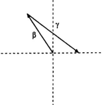
FIGURE 2. If$\lambda_{0}\leq 0,$ $|\beta|<|\gamma|$

Now we areready to prove the isomorphism theorem:

Theorem 36. Under the same assumption

as

in Theorem 34, the two

_fibmtions

$f:\partial E(r, \delta_{0})arrow S_{\delta_{0}}^{1}$, $\varphi:S_{r}^{2n-1}\backslash K_{r}arrow S^{1}$

are topologically isomorphic.

3. MIXED PROJECTIVE CURVES

Let $f(z,\overline{z})$ bc a rad-polar weighted homogeneous mixed polynomial with $z=$

$(z_{1}, \ldots, z_{n})\in \mathbb{C}^{n}$. Namely there exist integers $(q_{1}, \ldots, q_{n})$ and $(p_{1}, \ldots, p_{n})$ and positive intcgers $d_{r},$ $d_{p}$ such that

$\int(t\circ z, t\circ\overline{z})=t^{d_{r}}f(z,\overline{z})$, toz $=(t^{q\iota}z_{1}, \ldots, t^{q_{\hslash}}z_{n})_{\dot{\prime}}t\in \mathbb{R}^{+}$

$f(\rho\circ z,\overline{\rho\circ z})=\rho^{d_{\rho}}f(z,\overline{z})$, $\rho\circ z=(\rho^{P1}z_{1,\ldots)}\rho^{\rho_{n}}z_{n}),$ $\rho\in \mathbb{C},$ _$|\rho|=1$

.

This gives $\mathbb{R}^{+}\cross S^{1}$ action by

$(t, \rho)\circ z=(t^{q_{1}}\rho^{\rho_{1}}z_{1}, \ldots, t^{q_{n}}\rho^{p_{n}}z_{n})$, $t\rho\in \mathbb{R}^{+}\cross S^{1}$.

We say that $f(z,\overline{z})$ is strongly polar weighted homogeneous if$p_{j}=q_{j}$ for $j=$

$1_{:}\ldots,$ $n$

.

Then the associated $\mathbb{R}^{+}\cross S^{1}$ action on$\mathbb{C}^{n}$ is in fact thc $\mathbb{C}^{*}$ action which

is defined by

$(z, \tau)=((z_{1}, \ldots, n), \tau)\mapsto\tau oz=(z_{1}\tau^{\rho_{1}}, \ldots, z_{n}\tau^{p_{n}}),$ $\tau\in \mathbb{C}^{*}$.

We say $f(z,\overline{z})$ is strongly polar homogeneous if further the weights satisfies the

equalities$q_{j}=p_{j}=1$for any$j$

.

Astrongly polar weighted homogeneous polynomial

$f(z,\overline{z})$ satisfies the equality:

(6) $f((t, \rho)\circ z, \overline{(t,\rho)\circ z})=t^{d_{r}}\rho^{d_{p}}\int(z.\overline{z})$, $(t, \rho)\in \mathbb{R}^{+}\cross S^{1}$.

Assume that $f(z,\overline{z})$ is a strongly polar weighted homogeneous polynomial of

radial degree$d_{r}$ and ofpolar degree$d_{p}$ respectivcly and let $P=(p_{1}, \ldots,p_{n})$ be the

weight vector. Let $\overline{V}$ be the mixed affine hypersurface

$\tilde{V}=f^{-1}(0)=\{z\in \mathbb{C}^{n}|f(z,\overline{z})=0\}$

.

Let $\varphi$ : $S^{2n-1}\backslash Karrow S^{1}$ be the Milnor fibration with

$K=\tilde{V}\cap S^{2n-1}$ _and let $F$ be

the fiber. Recall that $\varphi(z)=\int(z,\overline{z})/|f(z,\overline{z})|$

.

Thus $F$ is defined by

We

can

equivalently consider the globalfibration$f$ : $\mathbb{C}^{n}-\tilde{V}arrow \mathbb{C}^{*}$

.

Thcn the Milnor

fiber is identified with the hypersurface $f^{-1}(1)$

.

The monodromy map $h$ : _{$Farrow F$}

(in either case) is defined by

$h( z)=(\exp(\frac{2p_{1}\pi i}{d_{p}})z_{1}, \ldots, \exp(\frac{2p_{n}\pi i}{d_{p}})z_{1})$ . We consider alsothe wighted projective hypersurface $V$ defined by

$V=\{(z_{1}:z_{2} :. . . :z_{n})\in \mathbb{C}\mathbb{P}(P)^{\iota-1}|f(z,\overline{z})=0\}$

whereCP$(P)^{n-1}$ is the weightedprojcctivespace defined by thcequivalenceinduced

by the above C’ action:

$z\sim w\Leftrightarrow\exists\tau\in \mathbb{C}^{*},$ _{$w=\tau\circ z$}

.

It is well-known that $\mathbb{C}\mathbb{P}(P)^{n-1}$ is an orbifold with at most cyclic quotient

singu-larities.

By (6), $z\in f^{-1}(0)$ and $z’\sim z$, then $z’\in f^{-1}(0)$

.

Thus the hypersurface

$V=\{[z]\in \mathbb{C}\mathbb{P}^{n-1}(P)|f(z)=0\}$ is well-defined. Consider the quotient map $\pi$ :

$S^{2n-1}arrow \mathbb{C}\mathbb{P}(P)^{n-1}$ or$\pi$ : $\mathbb{C}^{n}\backslash \{O\}arrow$ CIP$(P)^{n-1}$

.

Forthe brevity‘s sake,we denote

the restrictions $\pi|F:Farrow \mathbb{C}\mathbb{P}^{n-1}\backslash V$ and $\pi|K$ : $Karrow V$ by the same $\pi$

.

We are

interested in the topology of$V$ and the relation with the Milnor fibration.

3.1. Canonical orientation. It is well known that a complex analytic smooth

variety has

a

canonical orientation which

comes

from the complex structure (see

for example p.18, [7]$)$

.

Let $\tilde{V}=f^{-1}(0)$ be a mixed hypersurface. Take a point

$a\in\tilde{V}$. We say that a is a mixedsingularpoint of $\tilde{V}$

, ifa is acritical point of the

$mapp_{\sim}^{ing}f$ : $\mathbb{C}^{n}arrow$ C. Otherwise, a is a mixed regular point. Note that a point

a $\in V$ to be a regular point

as

a point of a real analytic variety is a necessary

condition but not a sufficient condition for the regularity as a point on a mixed variety. Recall that

a

is

a

mixed singular point ifand only if$df_{a}:T_{a}\mathbb{C}^{\tau\iota}arrow T_{f(a)}\mathbb{C}$

is surjective. This is equivalent tothe existencc of acomplex number $\alpha\in \mathbb{C}$ with

$|\mathfrak{a}|=1$ such that

$\overline{df}(a,\overline{a})=\alpha\overline{d}f(a,\overline{a})$ i.e., $\overline{\frac{\partial f}{\partial z_{j}}}(a,\overline{a})=(y\frac{\partial f}{\partial\overline{z}_{j}}(a,\overline{a}),$$.i=1,$

$\ldots,$

$\gamma\iota$

([23]). We assert that

Proposition 37. There is a canonical orientation on the smooth part

_of

a mixed

hypersurface.

Proof.

Take

a

regular point a $\in\tilde{V}$

.

The normal bundle $\mathcal{N}$ of $\tilde{V}\subset \mathbb{C}^{n}$ has a

canonical orientation so that $df_{a}$ : $\mathcal{N}_{a}arrow T_{f(a,\overline{a})}\mathbb{C}$ is an orientation preserving

isomorphism. This gives acanonicalorientation on $\tilde{V}$

so

that the ordered union of

the oriented frames $\{v_{1}, \ldots, v_{2n-2}, n_{1}, n_{2}\}$ of$T_{a}\mathbb{C}^{n}$ is the orientation of $\mathbb{C}^{b}$ ifand

only if $\{v_{1}, \ldots , v_{2,\iota-2}\}$ is

an

oriented frame of$T_{a}\tilde{V}$ where _{$\{n_{1}, n_{2}\}$} is

an

oriented

frame of normal vectors. $\square$

Consider amixed homogeneous hypersurface $\tilde{V}$

and let $V$ be the corresponding

mixed projective hypersurface.

Proposition 38. Let $a\in\tilde{V}\backslash \{O\}$

.

Then $a\in\tilde{V}$ is a mixed singular point

of

$\tilde{V}$

if

and only

_if

$\pi(a)\in V$ is a mixedsingular point.

3.2. Milnor fiberation and Hopf fiberation. Consider the Hopf fibration $\pi$ : $S^{2\tau\iota-1}arrow \mathbb{C}\mathbb{P}^{\tau\iota-1}$ and its restriction to the Milnor fiber _{$F=\{z\in S^{2r\iota-1}|f(z,\overline{z})>$}

$0\}$

.

Put $K=f^{-1}(0)\cap S^{2n-1}$ be the link. As $\int$ is polar weighted, it is easy to

see

that $\pi$ : $Farrow \mathbb{C}\mathbb{P}^{n-1}\backslash V$ is

a

cyclic covering of order $d_{p}$ and the covering

transformation is generated by the monodromy map

$h;Farrow F$, $z\mapsto\exp(\frac{2\pi i}{d_{p}})\cdot z$. Thus

we

have

Proposition 39. (1) $\chi(F)=d_{p}\chi(\mathbb{C}\mathbb{P}^{n-1}\backslash V)$.

(2) $\chi(\mathbb{C}\mathbb{P}^{\iota-1}\backslash V)=n-\chi(V)$ and $\chi(V)=n-\chi(F)/d_{p}$

.

(3) We have thefollowing exact sequence.

$1arrow\pi_{1}(F)arrow^{\pi\#}\pi_{1}(\mathbb{C}\mathbb{P}^{n-1}\backslash V)arrow Z/d_{p}Zarrow 1$

.

The following special

cases are

uscd later.

Corollary 40. (1) Suppose $n=2$

.

Then $K\subset S^{3}$ is a link. Put $7^{\cdot}$ be the

number

_of

the components. Then $V$ is $r$ points and $r$ and $\chi$ are related by

$\frac{\chi(F)}{d_{p}}=2-r\cdot$.

(2) Suppose$n=3$

.

_Then $V\subset \mathbb{P}^{2}$ is

a

curve

of

genus

$g$ and $1+2g= \frac{\chi(,F)}{d_{\rho}}$.

Remark 41. Let $f$ be a mixed polar weighted polynomial

of

two variables and let $r$ be the number

of

link components $S^{3}$. Let $s$ be the number

of

irreducible

components

_of

$f$. Then $r\geq s$. For example, For example, let $f(z_{1)}z_{2},\overline{z}_{1},\overline{z}_{2})=$

$-2z_{1}^{2}\overline{z}_{1}+z_{2}^{2}\overline{z}_{2}+tz_{1}^{2}\overline{z}_{2}$. Then

for

$t=0$, lkn$(f)=1=6$ and

for

$t=2,$ $s=1$ and

$1kn(f)=3$

.

Corollary 42.

_If

$d_{p}=1$, the projection $\pi$ : $Farrow \mathbb{C}\mathbb{P}^{n-1}\backslash V$ is a diffeomorphism.

The monodromymap $h:Farrow F$ givcs free $Z/d_{p}Z$ action on $F$

.

Thus usingthe

periodic monodromy argumcnt in [15], wcget

Proposition 43. The zeta

_function

_of

$h:Farrow F$ is _given by

$\zeta(t)=(1-t^{d_{p}})^{-\chi(F)/d_{p}}$.

In particular,

_if

$d_{\rho}=1,$ $h=id_{F}$ and$\zeta(t)=(1-t)^{-\chi(F)}$

.

3.3. Degree of mixed projective hypersurfaces. Suppose that$f(z,\overline{z})\in\Lambda t(q+$

$2r,$$q;n)$ be a stronglypolar homogeneous polynomial and let

$V=\{z\in \mathbb{C}\mathbb{P}^{n-1}|f(z,\overline{z})=0\}$.

We

assume

that the singular locus $\Sigma V$ of$V$ is either emptyor $co\dim_{R}\Sigma V\geq 2$. We

have observed that $V\backslash \Sigma V\subset \mathbb{C}\mathbb{P}^{n-1}$ is canonically oriented so that the union of

the oriented frame of$T_{P}V$, say $\{v_{1,\ldots,2(n-2)\}}?)$ and the frame of normal bundle

$\{w_{1}, w_{2}\}$ which is compatible with the local defining complex function $g_{j}$

on

the

affine chart$U_{j}=\{z_{j}\neq 0\}$ istheorientedframeof$\mathbb{C}\mathbb{P}^{n-1}$

.

(Recallthat

$g_{j}$ isamixed

Thus ithasafundamentalclass $[V]\in H_{2n-4}(V;Z)$ _{byBorel-Haefliger [4], The}

topo-logical degree of $V$ is the integer $d$so that $\iota_{*}[V]=d[\mathbb{C}\mathbb{P}^{7l-2}]$ where $l$, : $Varrow \mathbb{C}\mathbb{P}^{r\iota-1}$

$\mathbb{C}\mathbb{P}^{n-2}isthei.nclusion$ map and

$[\mathbb{C}\mathbb{P}^{n-2}]$ is the homology class ofa canonical hyperplane

Theorem 44. [22] The topological degree

_of

$V$ is equalto the polar degree_$q$

.

Namely the

_fundamental

class [V] corresponds to $q[\mathbb{C}\mathbb{P}^{n-2}]\in H_{2(n-2)}(\mathbb{C}\mathbb{P}^{n-1})$ by the inclu-sion mappin9 $\iota_{*}$

.

3.3.1. Residue

_{formula for}

amonic mixed polynomial. Let$g(w, \overline{w})=\sum_{a.b}c_{a,b}w^{a}\overline{w}^{b}$

be

a

mixed polynomial. Put $d= \max\{a+b|c_{a,b}\neq 0\}$ and we _call $d$ the radial degree of $g$. We say that $g$ is a monic mixed polynomial

of

degree $d$ if _$g$ has a

unique monomial of radial degrce $d$.

Lemma 45. Assume that$g(w,\overline{w})$ is a monic mixed polynomial

of

degree $d$ which

is written as

$g(w,\overline{w})=c_{0}(\overline{w})w^{q+r}+c_{1}(\overline{w})w^{q+r-1}+\cdots+c_{q+r}$

$c_{j}(\overline{w})\in \mathbb{C}[\uparrow\overline{v}],$ $rdcg_{\overline{w}^{C’}j}\leq\gamma\cdot,$$j=0,$

$\ldots,$$q+7^{\cdot}$ $c_{0}(\overline{w})=c_{0r}\overline{w}^{r}+\cdots+c_{00},$ $c_{0r}\neq 0$

with $d=q+2r$. Then

$\frac{1}{2\pi}l_{|w|=R}$Gauss$(g)d\theta=q$,

3.3.2. Mixedprojective

curves.

In this section, wc study basic examplesin the pro-jectivc surface $\mathbb{C}\mathbb{P}^{2}$

.

Thus we

assume

that $n=3$

.

We considcr projective

curves

of

degree $q$:

$C=\{[z_{1}:z_{2}:z_{3}]\in \mathbb{C}\mathbb{P}^{2}|f(z_{1}, z_{2}, z_{3})=0\}$

where $f$ is a strongly polar homogeneous polynomial with pdeg$f=q$

.

We have

seen

that the topological degree of$C$is $q$ by Theorem 44. The genus $g$ of$C$ is not

an

invariant of$q$

.

Recall that for

a

differentiable curve $C$ of genus $g$, embedded in

$\mathbb{C}\mathbb{P}^{2}$

, with the topological degree $q$,

wc

have the following Thom’s inequality, which

was conjectured by Thom and proved by for example Kronheimer-Mrowka [13]:

$g \geq\frac{(q-1)(q-2)}{2}$

wherethe right side number isthegcnus ofalgebraiccurvesof dcgree$q$, givenby the

Pl\"ucker _{formula. Recall that for a mixed strongly polar homogcneous polynomial,} the genus and the Euler characteristic ofthe Milnor fiber arc related as follows (

Corollary 40):

$g= \frac{1}{2}(\frac{\chi(F)}{q}-1)$

where

$F=\{(z_{1}, z_{2}, z_{3})\in \mathbb{C}^{3}|f(z_{1}, z_{2}, z_{3_{j}}\overline{z}_{1},\overline{z}_{2},\overline{z}_{3})=1\}$.

I. Simplicial polynomials. Wc consider the following simplicial polar

homoge-neous polynomials ofpolar degree $q$

.

$f_{s_{1}}(z,\overline{z})=z_{1}^{q+r}\overline{z}_{1}^{r}+z_{2}^{q+r}\overline{z}_{2}^{r}+z_{3}^{\eta+r}\overline{z}_{3}^{r}$

$f_{s_{2}}(z,\overline{z})=z_{1}^{q+r-1}\overline{z}_{1}^{r}z_{2}+z_{2}^{q+r-1}\overline{z}_{2}^{r}z_{3}+z_{3}^{q+r}\overline{z}_{3}^{r}$

$f_{\hslash_{J}^{a}}(z,\overline{z})=z_{1}^{q+r-1}\overline{z}_{1}^{\tau}.z_{2}+z_{2}^{q+r-1}\overline{z}_{2}.z_{3}+z_{3}^{q+r-1_{\overline{Z}_{3}^{z}Z_{1}}}$.

$f_{s4}(z,\overline{z})=z_{1}^{q+r+1}\overline{z}_{1}^{r}\overline{z}_{2}+z_{2}^{q+r+1}\overline{z}_{2}^{r}\overline{z}_{3}+z_{3}^{q+r}\overline{z}_{3}^{r}$

$f_{s_{5}}(z,\overline{z})=z_{1}^{q+r+1}\overline{z}_{1}^{r}\overline{z}_{2}+z_{2}^{q+r+1}\overline{z}_{2}^{r}\overline{z}_{3}+z_{3}^{q+r+1}\overline{z}_{3}^{r}\overline{z}_{1}$

Let $F_{s:}$ betheMilnor fiber of$f_{s_{i}}$ andlet $C_{s_{i}}$ be the corresponding projective

curves

for $i=1,$ $\ldots,$

$5$

.

First, the Euler characteristic ofthe Milnor fibers and the genera

arc

given

as

follows.

$\chi(F_{s}.)=q^{3}-3q^{2}+3q$_, $g(C_{s_{i}})= \frac{(q-1)(q-2)}{2},$ _$i=1,2.3$

$\chi(F_{s_{4}})=q(q^{2}+q+1)$, $g(C_{S4})= \frac{q(q+1)}{2}$

$\chi(F_{s_{5}})=q(q^{2}+3q+3)$, $g(C_{s_{4}})= \frac{(q+2)(q+1)}{2}$

In [21],

we

have shown that $C_{s_{1}}$ and $C_{s_{2}}$

arc

isomorphic to algebraic plane

curves

defined by the associated homogeneous polynomialsof degree $q$: $q_{s_{1}}(z)=z_{1}^{q-1}z_{2}+z_{2}^{q-1}z_{3}+z_{3}^{q}$

$g_{S2}(z)=z_{1}^{q-1}z_{2}+z_{2}^{q-1}z_{3}+z_{3}^{q}$.

We also expect that $C_{s_{3}}$ is isotopic tothe algebraic

curve

$z_{1}^{q-1}z_{2}+z_{2}^{q-1}z_{3}+z_{3}^{q-1}z_{1}=0$,

as

the genus of $C_{s_{3}}$ suggests it (see also [21]).

II. We consider the followingjoin type polar homogeneous polynomial. $h_{j}(z,\overline{z})=g_{j}(w^{-}w)+z_{3}^{q+r_{\overline{Z}_{3}^{r}}}$,

$g_{j}(w,-w)=(w_{1}^{q+.7}\overline{w}_{1}^{j}+w_{2}^{q+j}\overline{w}_{2}^{j})(\uparrow v_{1}^{r-j}-\alpha w_{2}^{r-j})(\overline{w}_{1}^{r-j}-\beta\overline{w}_{2}^{r-j})$, $0\leq j\leq r$.

($\alpha,$$\beta\in$ C’

are

generic.) The the Milnor fiber $F_{g_{g}}$ of $g_{j}$ is connected. The link

componentnumber of$g=0$islkn$(g)=q+2(,.-j)$. Thus$\chi(F_{g_{j}})=q(q-2+2(’\cdot-j))$

by Corollary 40 and $g= \frac{(q-1)(q-2+2(r-j))}{2}$

.

In particular, taking$q=2$, we obtain

$g=r-j$

and thus

Corollary46. Forany smooth

_surface

$S$

of

genus_$g$, thereis an embedding$S\subset \mathbb{C}\mathbb{P}^{2}$

so that the degree

_of

$S$ is 2.

We observe that the

case

$q=1$ gives only the trivial

casc

$g=0$ in this family. 3.4. Twisted join type polynomial. In this section,we introducc a

new

class of mixedpolarweighted polynomials which we

use

toconstruct

curves

withembedded

degree 1. For further detail,

see

[22]. Let $f(z,\overline{z})$ be apolar weighted homogeneous

polynomial ofn-variables $z=(z_{1}, \ldots, z_{n})$

.

Let $Q={}^{t}(q_{1},$

$\ldots,$$q_{n}),$ $P=\downarrow(p_{1}, \ldots,p_{n})$ be the radial and polar weight respectively and let $d,$ $q$ be the radial and polar

${}^{t}(p_{1}/q,$ $\ldots,p_{n}/q)$ the normalized mdial weights and the normalized polar weights

respectively.

Consider

the mixed polynomial of (n$+$ l)-variables:

$g(z,\overline{z}, w.\overline{w})=f(z,\overline{z})+\overline{z}_{n}w^{a}\overline{w}^{b}$, $a>b$

.

Consider thc rationalnumbers $\overline{q}_{n+1},\overline{p}_{n+1}$ satisfying

$\frac{q_{n}}{d}+(a+b)\overline{q}_{\iota+1}=1$, _{$- \frac{p_{n}}{q}+(a-b)\overline{p}_{\iota+1}=1$}.

We

assume

that $q_{?t}<d$sothat $\overline{q}_{\iota+1},,\overline{p}_{r\iota+1}$

are

positive rationalnumbers. The

poly-nomial $g$ is a polar weighted homogeneous polynomial with the normalized radial

and polar weights $\overline{Q’}=L(q_{1}/d, \ldots , q_{n}/d,\overline{q}_{\tau+1})$ and $\overline{P’}={}^{t}(p_{1}/q,$

$\ldots,$$p_{n}/q,\overline{p}_{n+1})$

respectively. The radial and polar degrec of $g$ are given by lcm$(d. denom(\overline{q}_{n+1}))$

and lcm$(q, dcnorn,(\overline{p}_{n+1}))$ wherc$dr^{I},\gamma\iota om(x)$ is the dcnominator of$\prime f’\in \mathbb{Q}$. Wecall,$q$ $a$

twistedjoin

_of

$\int(z,\overline{z})$ and$\overline{z}_{n}w^{a}\overline{w}^{b}$

.

We saythat

9 is apolar weighted homogeneous

polynomial of twistedjoin type. A twisted join type polynomial behavesdifferently than the simplejoin type, as

wc

will

see

below.

We recall that $f(z,\overline{z})$ is callcd to bc l-convenient ifthe restriction of $f$ to each coordinate hyperplane $f_{i}$ _{$:=f|_{\{z_{i}=0\}}$} is non-trivial for $i=1,$

$\ldots,$$n$ ([23]) Lemma 47. Assume that $n\geq 2$ and $f$ is l-convenient. Then

$\phi_{\#}:\pi_{1}((\mathbb{C}^{*})^{n}\backslash F_{f}^{*})\cong Z^{n}\cross Z$

is an isomorphism where $\phi$ is the canonical mapping

$\phi:(\mathbb{C}^{*})^{n}\backslash F_{f}^{*}arrow(\mathbb{C}^{*})^{n}\cross(\mathbb{C}\backslash \{1\})$

defined

by $\phi(z)=(z, f(z,\overline{z}))$ and $F_{f}^{*}$ $:=f^{-1}(1)\cap(\mathbb{C}^{*})^{n}$

.

Put $F_{f_{n}}:=f_{n}^{-1}(1)=F_{f}\cap\{z_{n}=0\}\subset \mathbb{C}^{n-1}$ with $f_{\mathcal{T}l}:=f|_{\mathbb{C}^{n}\cap\{z_{n}=0\}}$

.

Theorem 48. [22] Assume that $n\geq 2$ and $f$ is l-convenient and$g(z,\overline{z}, w,\overline{w})$ is

a

twistedjoin polynomial as above. Then

(1) the Milnor

_{fiber of}

$g,$ $F_{g}=g^{-1}(1)$, is simply connected.

(2) The Euler charactentstic

_of

$F_{9}$ is given by the formula;

$\chi(F_{g})=-(0-b-1)\chi(F_{f})+(c\prime_{l}-b)\chi(F_{f_{n}})$.

3.4.1. Construction

_of

a family

_of

mixed curves with polar degree $q$

.

Now we

are

ready to construct akey family ofmixed

curves

with embedding degree $q$. Recall

the polynomial:

$h_{q.r,j}(w,\overline{w}):=(z_{1}^{q+j}\overline{z}_{1}^{j}+z_{2}^{q+j}\overline{z}_{2}^{j})(z_{1}^{r-j}-\alpha z_{2}^{r-j})(\overline{z}_{1}^{r-j}-\beta\overline{z}_{2}^{r-j}))$ _{$w=(z_{1}, z_{2})$}. $h_{q,r},.’(w, w-)$ is l-convenientstronglypolarhomogeneous polynomialwiththe radial

degrce $q+r$ and thc polar degree $q$ respectively. The constants $\alpha,$$\beta$ are generic,

For this, it suffices to

assume

that $|\alpha|,$$|\beta|\neq 0,1$ and $|\alpha|\neq|\beta|$. Consider the twisted join polynomial of3 variables $z_{1},$$z_{2},$$z_{3}$:

$s_{q,r,j}(z,\overline{z})=h_{q,r,g}(w^{-}w)+\overline{z}_{2}z_{3}^{q+r}\overline{z}_{3}^{r-1}$ , $z=(z_{1}, z_{2}, z_{3})$.

Let $F_{q,r,j}=s_{q,r,j}^{-1}(1)\subset \mathbb{C}^{3}$ be the Milnor fiber and let $S_{q,r,j}\subset \mathbb{P}^{2}$ be the

corre-sponding mixed projective

curve:

$S_{q,r,j}=\{[z]\in \mathbb{P}^{2}|s_{q,r,j}(z,\overline{z})=0\}$.

Note that $S_{q,r,j}$ is a smooth mixed

curvc.

The following describes the topology of $F_{q,,.,j}$ and $S_{q.?\cdot,j}$

.

Theorem 49. (1) The Euler chamcteristic

_of

the Milnor

_fiber

$F_{q,r,j}$ is given

$by$:

$\chi(F_{q,r,j})=q(q^{2}-q+1+2(r-j))$

.

(2) The genus

_of

$S_{q,’\cdot,j}$ is given by:

$g(S_{q.r,j})= \frac{q(q-1)}{2}+(r-j)$

Proof.

Let $H_{q,r,j}=h_{q,,.,j}^{-1}(1)$

.

Then by Corollary 40,

$\chi(H_{q,r,j})=-q(q-2+2(r-j))$

$\chi(H_{q,r,j}\cap\{z_{2}=0\})=q$

and thc assertion follows from Theorcm 48. 口

3.4.2. Mixed

curves

with polar degree 1. We considcr thc

case

$q=1,$$j=0$:

$\{\begin{array}{ll}f\iota(w, w-) :=(z_{1}+z_{2})(z_{1}^{r}-\alpha z_{2}^{r})(\overline{z}_{1}^{r}-\beta\overline{z}_{2}^{r})f_{r}(z,\overline{z}) :=h(w,\overline{w})+\overline{z}_{2}z_{3}^{r+1}\overline{z}_{3}^{r-1}S_{r} :=\{[z]\in \mathbb{P}^{2}|f_{r}(z,\overline{z})=0\}.\end{array}$

Corollary 50. Let $S_{r}$ be the mixed

curve

as

above. Then the embedding degree

of

$S_{r}$ is 1 and the genus

of

$S_{r}$ is $r$

.

Proof.

Let $F_{r}=f^{-1}(1)$ be theMilnorfiberof$f_{r}$

.

ByTheorem 48,

we

have$\chi(F_{r})=$

$2r+1$

.

Thus by Corollary 40, the assertion follows immediately. 口

Remark 51. $h,(w, w-)$ can be replaced by $(z_{1}^{r+1}-z_{2}^{r+1})(\overline{z}_{1}-\beta\overline{z}_{2}^{r})$ without changing

the topology.

REFERENCES

[1] N. A‘Campo. Lafonction zeta d‘urlemonodromie. Comm. Math. Helv., 50:539-580, 1975.

[2] R. Benedetti and J.-J. Risler. Real algebraic and semi-algebraic sets. Actualit\’es

Math\’ematiques. [Current MathematicalTopics]. Hermann, Paris, 1990.

[3] A. Bodin and A. Pichon. Meromorphic functions, bifurcation sets and fibred links. Math.

Res. Lett., 14(3):413-422, 2007.

[4] A. Borel and A. Haefliger. Laclasse d‘homologie fondamentale d‘un espaceanalytique. Bull.

Soc. Math. Phance, 89:461–513, 1961.

[5] J. L.Cisneros-Molina. Join theorem forpolarweighted homogeneoussingularities. In

Singu-larities II, volume475 of Contemp. Math., pages 43-59. Amer, _{Math. Soc., Providence, RI,}

2008. [6]

[7] P. Griffiths and J. Harris. Principles _of algebraic geometry. Wiley Classics Library. John

Wiley &Sons Inc., New York, 1994. Reprint of the 1978 original.

S. M. GuseYn-Zade, I. Luengo,andA.Melle-Hern\’andez. Zetafunctions of germsof

meromor-phic functions, and the Newton diagram. Funktsional. Anal. i Pnlozhen., $32(2):26-35,$ 95,

1998.

[8] S. M. GuseIn-Zade, I. Luengo, and A. Melle-Hern\’andez. On the topology of germsof

mero-morphicfunctions and its applications. Algebm i Analiz, $11(5):92-99$, 1999.

[9] H. Hamm. Lokale topologische Eigenschaften komplexerR\"aume. Math. Ann., 191:235-252,

1971.

[10] H. A. Hamm and D. T. L\^e. Unth\’eor\‘eme de Zariski du typede Lefschetz. Ann. Sci. \’Ecole

Norm. Sup. (4),6:317-355, 1973.

[11] M. Kato andY.Matsumoto.On theconnectivityoftheMilnorfiber ofaholomorphicfunction

at acritical point. In Manifolds–Tokyo 197S (Proc. Intemat. Conf., Tokyo, 197S), pages

[12] A. G. Kouchnirenko. Poly\‘edres de Newton et nombres de Milnor. Invent. Math., 32:1 31, 1976.

[13] P. B. Kronheimer and T.S. Mrowka. The genus of embedded surfacesin theprojective plane.

Math. Res. Lett., 1(6):797.808, 1994.

[14] F. Michel, A. Pichon, andC. Weber. The boundary of the Milnor fiber ofHirzebruchsurface

singularities. In Singularity theory, pages 745760. World Sci. Publ., Hackensack, NJ, 2007.

[15] J. Milnor. Singularpoints _ofcomplexhypersurfaces. AnnalsofMathematicsStudies, No. 61.

Princeton University Press, Princeton, N.J., 1968.

[16] J. Milnorand P. Orlik. Isolatedsingularities definedby weighted homogeneous polynomials.

Topology, 9:385-393, 1970,

[17] M.Oka. On the resolution ofthe hypersurfacesingularities.In Complexanalyticsingulart,ties,

volume 8of Adv. Stud. Pure Math.,pages 405-436. North-Holland, Amsterdam, 1987.

[18] M. Oka. Principal zeta-function ofnondegenerate complete intersection singularity. J. Fac.

Sci. Univ. Tokyo Sect. IA Math., 37(1):11-32, 1990,

[19$|$ M. Oka. On the topologyoffull nondegenerate complete intersection variety. Nagoya Math.

J., 121:137..148, 1991,

[20] M. Oka. Non-degenerate complete intersectionsingulanty. Hermann, Paris, 1997. [21] M. Oka. Onmixed Brieskornvariety. Comtemporary Math., 538,389-399,20, 2011

[22] M. Oka. On rnixed planecurves ofpolardegree 1. Proceeding _ofthe Centre_forMath. and its

applications, Australian National Univ., 43, 67-74, 2010

[23] M. Oka. Topologyofpolarweighted homogeneous hypersurafces. Kodai Math. $J_{)}$31(2):163

182, 2008.

[24] M. Oka. Non-degenerate mixedfunctions. KodaiMath. J., 33(1):1 62, 2010.

[25] A. Pichon. Real analyticgerms $f\overline{g}$andopen-book decompositions of the 3-sphere. Intemat.

J. Math., 16(1): 1-12, 2005.

[26] A. Pichon and J. Seade. Real singularities and operi-book decompositions of the 3-sphere.

Ann. Fac. Sci. Toulouse Math. (6), 12(2):245265, 2003.

[27] M. A. S. Ruas, J. Seade, and A. Verjovsky. Onreal singularities with a Milnor fibration. In

Trends in singulanties, Trends Math., pages 191-213. Birkhauser, Basel, 2002.

[28] J. Seade. Open book decompositions associatedtoholomorphic vectorfields. Bol. Soc. Mat. Mexicana (3), $3(2):323$ 335, 1997.

[29] J. Seade. On the topology ofhypersurface singularities. In Real and complex singulamties,

volume 232 of Lecture Notes in Pure and Appl. Math., pages 201 205. Dekker, New York,

2003,

[30] A. N.Varchenko. Zeta-functionof monodrornyand Newtonsdiagram. Invent. Math.,

37:253-262, 1976.

[31] J. A. Wolf. Differentiable fibre spaces and mappings compatible with Riemannian metrics.

Michigan Math. J., 11:65-70, 1964.

DEPARTMENT oP _MATHEMATICS

TOKYO UNIVERSITY OF SCIENCE

26 $w_{AKAM}$lYA-C110, $s_{HINJUKU-KU}$

TOKYO 162-8601