Strategic location model for oil spills response installations considering oil transportation (New Trends of Numerical Optimization in Advanced Information-Oriented Society)

全文

(1)31 31. Strategic location model for oil spills response installations considering oil transportation Rafael Pedro Longhi LORDE, Universidade Federal do Rio de Janeiro. 1. lntroduction. Although every oil & gas plant should avoid oil spills, it is impossible to have a guarantee that no incident will occur. For instance, in 2010, Deepwater Horizon oil spill occurred in Golf of Mexico, and,. in 2011, another occurred in Campos Basin in Brazil. These events show the importance of studies related to the problems caused by oil spills on environment and means to make contingency. To avoid impacts of an oil spill in offshore oil & gas production, it is necessary to maintain vessels. in stand‐by with protection equipment near oil production maritime units. Determination of location of these vessels is complex, as it is important to attend any oil spill in Iess than a critical time, according to regulations. The main objective of this work is similar to the one presented by Costa (2007), there is, implement an optimization model for strategic decision of the location of these facilities. It is a covering problem, where each vessel works Iike a warehouse and accident points are clients.. This work presents an implementation similar lakovou, Douligeris, lp. e. Korde (1996) model, which. is. However, now this work also intends to consider oil transportation in the model. This work assumes that oil would have constant speed and would spread in a radius trajectory.. 2. Literature review. lakovou, Douligeris, lp. e. Korde (1996) proposed a mixed linear integer mathematical programing. model to define Iocations of oil response installations that is the base for this work. This model was. also on experiments of Costa (2007). In this model, main objective is to determine the candidate Iocations for warehouse opened, the quantity of equipment stored at them and quantity of equipment that each of this warehouses would be responsible to send to maritime units in case of oil spill. On model input, we should provide costs for opening a new facility, operational costs to maintain equipment in facility, transportation costs in case of emergency, demands in case of accident, duration of trips between each warehouse location candidate and clients, critical time to reach accident zone and demands in case of accident.. Model considers that probability of having two accidents at same time is very Iow, so response system capacity considers only one accident per scenario. Model is as follows: Sets. I. J. Candidate Iocations for vessel (warehouse) Types ofequipment.

(2) 32 Client Iocations (maritime unit location). K. Parameters. Cost to open warehouse on location i Cost to maintain equipment j on location. \alpha_{i}. \beta_{ij}. i. \gamma_{j}. Cost to transport equipment j per unit of time. \tau_{ik}. Travel time between warehouse i and location k. C_{ij} D_{jk} A_{ik}. Capacity of location i for equipmentj Demands of equipmentj on discretization l of client k 1 if travel time of route between location i and point l of client. M. Number sufficiently big.. k circumference takes less than critical time. Variables. Quantity of equipmentj stored at vessel i 1 if vessel i opens Quantity of equipmentj sent from vessel i to point l in client k, that is in position p in route. x_{ij} y_{i}. z_{ijk}. min. \sum_{i}\alpha_{i}y_{i}+\sum_{i}\sum_{j}\beta_{ij}x_{ij}+\sum_{i}\sum_{j}\sum_ {k}\gamma_{j}\tau_{ik}z_{ijk}. (1). S.t.. \chi_{ij}\leq C_{ij}y_{i}. \forall iEI,jEJ. (2). \sum_{i}z_{ijk}\geq D_{ik}. \forall j\in J, kEK. (3). \forall i\in I,jEJ, k\in K \forall i\in I,j\in J, k\in K. (4) (5) (6) (7). z_{ijkl}\leq x_{ij} z_{ijkl}\leq MA_{ikl} x_{ij},. z_{ijk}\in \mathbb{Z}^{+}. y_{i}\in\{0,1\}. \forall i\in I,j\in J, k\in K \forall i\in I. Objective function minimizes opening costs, operational costs to maintain equipment on warehouse and transportation costs for scenarios concerning accidents on each of the risk points. Constraint (2) guarantees that only opened facility can store any product, until its capacity. Constraint (3) ensure attendance of demands of each client. Constraint (4) deals with capacity of warehouse. Constraint (5) makes possible only trips between warehouse and clients that take Iess than critical time. Rest of constraints deal with definition of variables..

(3) 33 3. Model. On this work, we propose modifications on model proposed by lakovou, Douligeris, lp e Korde (1996) to consider oil transportation. Therefore, now we does not need to attend not only original location of clients, but also all border of area affected by oil spill. We adopt two different approaches: in a simpler model, we discretize this border in points and treat them exactly as previous model; and in a more advanced model, we also define order of stops during attendance of points.. 3.1 Discrete model considering oil transportation In this case, oil suffers transportation after spilldue to wind and maritime currents. Therefore, now it is necessary to reach not only oil spill origin, but also all border of affected area within critical time. For simplification, model considers that oil spreads is in a radial trajectory, with constant speed w , in all directions. In critical time (T_{crit}) , oil would cover an area inside a circle with. r=wT_{crit} .. (8 \}. Therefore, now constraints of problem have to impose that all vessels could reach all points of this circumference within. T_{crit}.. For example, for a point required to reach oil is. B. in circumference, assuming that vessels operate with speed. r( \theta)=\frac{v}{dist}.. v. , time. (9 \}. Where dist is the distance between warehouse and any point in circumference, as in Figure 1. with coordinates (a, b) , and client is represented by point C, with coordinates (c, d) . We should attend all points of discretized circumference formed by oil spread, for example point B. Warehouse is represented by point. A,. t\prime\theta0,\bulet^{e -e }C=(c_{k}.d_{k}). B=(x.y) \prime'r=wT_{\iota\tau it} dist ’. \bulet^{\prime^{t} \prime\prime A=(a_{i\prime}b_{i}) Figure 1. Distance traveled by vessel.. Expressing. x. and. y. in function of \theta , we have:.

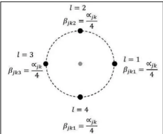
(4) 34 x=c_{k}+r\cos(\theta). (10}. y=d_{k}+r\sin(\theta). (11). To calculate distance between A and B , we proceed as following: (12). dist=\sqrt{(x-a_{i})^{2}+(y-b_{i})^{2}} Considering that vessel has a speed. v. , model only allows routes performed bellow critical time.. Therefore, now matrix of allowed routes would have following values:. \{begin{ar y}{l A_{ikl}=1,if\rac{dist}{v\leqT_{crit} A_{ikl}=0,if\rac{dist}{v>T_{crit} \end{ar y}. (13}. For simplification, model discretizes circumference in a set of points, which vessel would have to. attend.. \beta_{jkl}. For. N. discretization,. each. l. points. would. have. following. demands. :. \beta_{jkl}=\frac{\alpha_{jk} {N}. (14). For example, if the quantity of discretization is four, clients considered in this model would be as in Figure 2.. l=2. \beta_{jk2}=\frac{\alpha_{jk} {4}. \prime\prime\prime^{- \bullet-}.-s_{N} l=3 I. sss. \prime t. \beta_{jk3}=\frac{ lpha_{jk}4\bulet\bulet,\bulet\prime\backsl h \backsl h\backsl h\primes_{N1',\primes_{-}\prime}\sim. \bulet\simpr e\prime\prime\prime\bta_{jk1}=\frac{ lpha_{jk}4l=1 l=4. \beta_{jk1}=\frac{\alpha_{jk} {4} Figure 2. Example of clientsfor new model, considering circumference divided in 4 sections.. With these new assumptions, model is now as follows:.

(5) 35. Sets. K. Candidate Iocations for vessel (warehouse) Types of equipment Client Iocations (maritime unit location). L. Points of discretized circle. I. ]. Parameters. \gamma_{j}. Cost to open warehouse on location i Cost to maintain equipment j on location i Cost to transport equipment j per unit of time. \tau_{ikl}. Travel time between warehouse i and discretization l of. C_{ij} D_{jk} A_{ikl}. Capacity of location i for equipmentj Demands of equipmentj on discretization l of client k 1 if travel time of route between location i and point l of client. M. Number sufficiently big. In this case, we consider it as \max(C_{ij}). \alpha_{i}. \beta_{ij}. location k. k circumference takes less than critical time. Variables. Quantity of equipmentj stored at vessel i 1 if vessel i opens Quantity of equipmentj sent from vessel i to point l in client k, that is in position p in route. \chi_{ij} y_{i}. z_{ijkl}. min. \sum_{i}\alpha_{i}y_{i}+\sum_{i}\sum_{j}\beta_{ij}x_{ij}+\sum_{i}\sum_{j}\sum_ {k}\sum_{l}\gamma_{j}\tau_{ikl}z_{ijkl}. (15 \}. s.t.. \chi_{ij}\leq C_{ij}y_{i}. \sum_{i}z_{ijkl}\geq D_{ikl} \sum_{\iota}z_{ijkl}\leq x_{i } \sum_{\iota}z_{ijkl}\leq MA_{ikl}. x_{ijt}z_{ijk}\in \mathbb{Z}^{+} y_{i}\in\{0,1\}. \forall iEI,jEJ. (16). \forall j\in J, k\in K, l\in L. (17 \}. \forall i\in I,j\in J, k\in K. (18). \forall i\in I,jEJ, k\in K. (19). \forall i\in I,j\in J, k\in K. (20) (21 \}. \forall i\in I.

(6) 36 Objective function minimizes opening costs, operational costs to maintain equipment on. warehouse and transportation costs for scenarios concerning accidents on each of the risk points. Constraint (16) guarantees that onlyopened facility can store any product, until its capacity. Constraint. (17) ensure attendance of demands of each point l of each client circumference. Constraint (18) deals with capacity of warehouse, imposing that, for each scenario of oil spill, sum of deliveries from a warehouse to circumference points should be lower than this warehouse capacity. Constraint (19) makes possible only trips between warehouse and points of circumference that take Iess than critical time. Rest of constraints deal with definition of variables.. 3.2 Discrete model considering oil transportation and vessel routing In previous approach, we only allowed clients reached before critical time in a directly route from vessel original position. It does not take into account that vessel can attend several clients before arriving, resulting in much more time than expected. To deal with it, we also propose a more complex model, which can decide vessel routes and arrival times. Sets. I. J K. L. Candidate Iocations for vessel (warehouse) Types ofequipment Client Iocations (maritime unit location) Points of discretized circle, zero representing routes that come from origin. Parameters. T_{kl_{1}l_{2}}. Cost to open warehouse on location i Cost to maintain equipment j on location i Cost to transport equipment j per unit of time Travel time between points in discretization l_{1} and l_{2} of. \tau_{ikl}. Travel time between warehouse i and discretization l of. C_{ij} D_{jk}. Capacity of location i for equipmentj Demands of equipmentj on discretization l of client. CT. Critical time. \alpha_{i}. \beta_{ij} \gamma_{j}. location k location k. k. Variables. x_{ij} y_{i}. z_{ijkl}. a_{ikl_{1}l_{2}} t_{ikl}. Quantity of equipmentj stored at vessel i 1 if vessel i opens Quantity of equipmentj sent from vessel i to point l in client k, that is in position p in route Vessel i performs trip between points l_{1} and l_{2} of client k Time when point l of client k is attended by vessel i.

(7) 37 q_{ijkl_{1}l_{2}}. Quantity of equipmentj onboard on vessel between points l_{1} and l_{2} of client k. y_{i}+\sum_{i}\sum_{i}\sum\sum_{ji kl}\sum_{k}\sum_{l^ _{1} \sum_{l 2} \gam a_{j}T_{kl T}l_{2}q_{ijkl_{1}l_{2}+\sum^{}\sum_{j}^\beta_{ij}\sum_{k} ^{x_ij}\sum_{l}^+\gam a\tuqijk0. (22 \}. s.t.. \chi_{ij}\leq C_{ij}y_{i}. \forall i\in I,j\in J. (23). \forall j\in J, k\in K, l\in L. (24 \}. \forall i\in I,jEJ, k\in K. (25). \forall i\in I, k\in K. (26). \sum_{l_{3}\inL}a_{ikl_{2}l_{3} \leq\sum_{l_{1}\inL\prime}a_{ikl_{1}l_{2}. \forall i\in I, k\in K, l_{2}\in L. (27). a_{ik\iota l}\leq 0. \forall i\in I, k\in K, lEL ’. t_{ikl_{1}}+T_{kl_{1}l_{2}}-t_{ikl_{2}}=M_{1}(1-a_{ikl_{1}l_{2}}) t_{ik0}+\tau_{ikl}-t_{ikl_{2}}=M_{1}(1-a_{ikl_{1}l_{2}}). \forall i\in I, k\in K, l_{1}\in L, l_{2}\in L \forall i\in I, k\in K, l_{2}\in L. (28) (29 \} (30). t_{ikl_{2} \leq M_{1}\sum_{l_{1}\in L'}(1-a_{ikl_{1}l_{2} ). \forall i\in I, k\in K,. \sum_{i\in l}z_{ijkl}\geq D_{jkl} \sum_{l\in L}z_{ijkl}\leq x_{i } \sum_{l\in L}a_{ik0l}\leq 1. t_{ikl}\leq CT. z_{ijkl_{2} \leqM_{2}(\sum_{l 1}\inL^{\backslash}a_{ikl_{1}l_{2}) a_{ikl_{1}l_{2} \leq\sum_{j}z_{ijkl_{1}. x_{ij}\in \mathb {Z}^{+}q_{i_{\dot{j} kl_{1}l_{2} -x_{i }\leq M_{3}(1- a_{ikl_{1}l_{2} ) z_{ijkl}t_{ikl}t, q_{ijkl_{I}l_{2}}, r_{ijkl}\in \mathbb{R}^{+} y_{i}, a_{ikl_{1}l_{2}}, b_{ikl}\in\{0,1\}. l_{2}\in L'. (31). \forall i\in I, kEK, l\in L. (32). \forall i\in I,j\in J, k\in K, l_{2}\in L. (33 \}. \forall i\in I, k\in K,. l_{1}EL', l_{2}\in L. (34). \forall i\in I,j\in J, k\in K, l_{1}\in L', l_{2}\in L \forall i\in I,j\in J, k\in K \forall i\in I, k\in K, l_{1}\in L, l_{2}\in L, l\in L. (37). \forall i\in I, k\in K, l_{1}\in L, l_{2}\in L, l\in L. (38 \}. (36)(35). Objective function minimizes opening costs, operational costs to maintain equipment on warehouse and transportation costs for scenarios concerning accidents on each of the risk points.. Constraint (23) guarantees that only opened facility can store any product, until its capacity. Constraint (24) ensures attendance of demands of each point l of each client circumference. Constraint (25) allows deliveries only in case of warehouse has enough equipment for it and it is opened,. Constraint (26) ensures that every trip have only one beginning. Constraint (27) ensures that trips can occur only in arcs where vessel already arrived at first client. Constraint (28) ensures that trips cannot occur in arcs beginning and ending on same point..

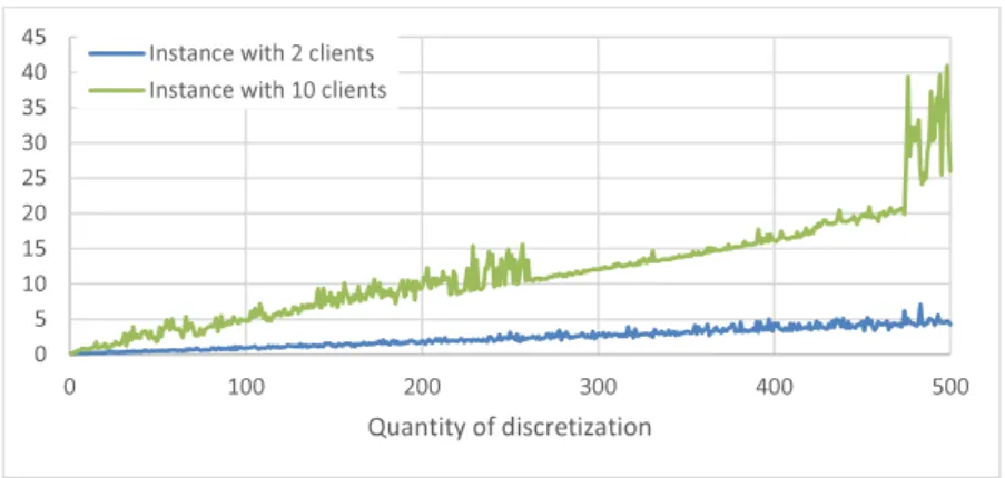
(8) 38 Constraints (29) and (30) calculate arrival time at each client and on first client of route, respectively. Constraint (31) makes time be equal to zero on departing time of vessel and on cases there is no route occurring. Constraint (32) ensures that only points reached before critical time can be attended.. Constraint (33) ensures that deliveries only occur in points attended by a route. Constraint (34) ensures that there is only trips in case of necessity of deliveries. Constraints (35) calculates quantity of equipment onboard on every stop of vessel, which we consider equal to the original quantity of goods in the vessel. Other constraints deal with definition of variables.. 4. Experiments. Experimentation used same instance as Costa (2007). For experiments, we implemented model proposed by lakovou, Douligeris, lp e Korde (1996), as well as ourtwo model considering oil transportation. For simple model considering oil transportation, experiments considered different choices for quantities of discretization, ranging from lto 500. For more complex model, we also did this, but with quantities of discretization in a range from lto 10. We considered instance with two sizes, one with only first two clients and another one with a1110 clients. Implementation was in Python, with Pulp library. Optimal solution was obtained using Gurobi solver for all models and also COIN‐OR for lakovou, Douligeris, lp e Korde (1996) model. Computer used has following specification: Processor Intel core 172. 20GHz, 16GB memory RAM.. 5. Results. 5.1 Model without oil transportation For instance with 10 clients, model constructed has 534 variables and 1088 constraints. According. to optimal solution found by solvers, Iocations4 and 5 will open. For this instance, GUROBI obtained solution in 0. 42s and COIN‐OR in 0. 39s . Considering also time demanded to process results and make output in Excel, time required was 1.. 92s. and 1.. 90s ,. respectively.. 5.2 Model with oil transportation Time required for solving problem, for different quantities of discretization, is in Figure 3. Model can achieve solution in acceptable computational time for any choices for discretization. Cases with more number of points lead to a better approximation of problem, but it makes problem more difficult to solve and it takes more time to reach optimal result. However, even in this cases, demanded time is not so big..

(9) 39 45 40 35 30 25 20 15. 10 5. 0 0. 100. 200. 300. 400. 500. Quantity of discretization. Figure 3. Computational time required for solve problem with oil transportation.. As seen on Figure 4 and Figure 5, quantity of variables and constraints of each problem have a great increase when number of divisions is bigger.. 300000. 250000. —Instance with 2 clients —Instance with 10 clients. 20000 15000 10000 5000. 0. 100. 200. 300. 400. 500. Quantity of discretization. Figure 4. Number of variables for model with oil transportation.. 300000 25000 20000 15000 10000 5000. 0. 100. 200. 300. 400. Quantity of discretization. Figure 5. Number of constraints for model with oil transportation.. 500.

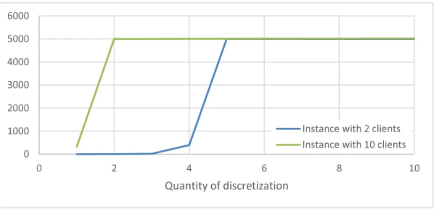
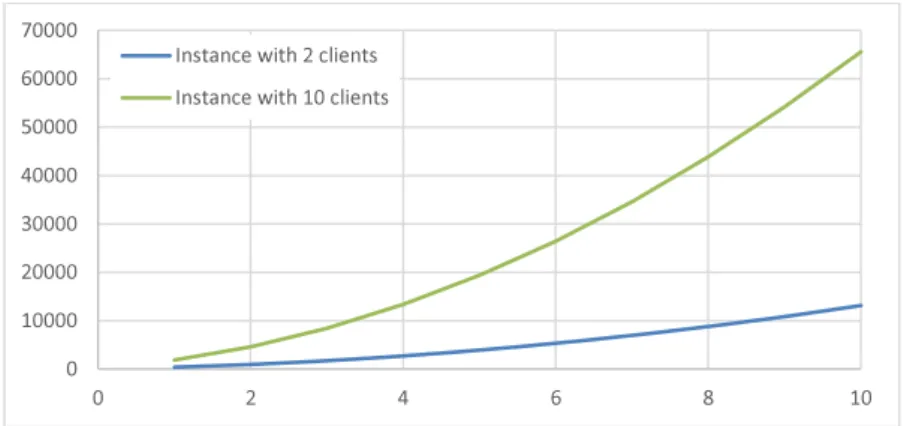
(10) 40. 5.3 Model with oil transportation and routing Time required for solving problem, fordifferent quantities of discretization, is in Figure6. As model is much more complex than previously, time required is bigger, then we defined a time limit for solver of 5000s. ln case this time is reached, solver stops processing and gives current results, which would be not optimal solution. In Figure 7, we present gap obtained in each of the results. It would be zero in cases we reached in optimal solution, and worse in cases it is near 1. This problem is much more complex than previous, resulting in bigger computational times and solution far from optimality as number of discretization increases.. 6000 5000 4000 3000 2000 1000 0. 0. 2. 4. 6. s. 10. Quantity of discretization. Figure 6. Computational time required for solve problem with oil transportation and routing.. 100 90. -. lnqtancp with 7 rlipnt \varsigma. 80 70. 60 50 40 30. 20 10 0 0. 2. 4. 6. 8. 10. Quantity of discretization. Figure 7. Gap for problem with oil transportation and routing. Increase on time can be explained by dimension of problem, as can be seen on numberofvariables. and constraints of on Figure 8 and Figure 9..

(11) 41 41. 70000. 60000 50000. 40000 30000. 20000 10000. 0 0. 2. 4. 6. s. 10. Figure 8, Number of variables for model with oil transportation and routing.. 90000 80000. —Instance with 2 clients. 70000 60000 50000 40000 30000. 20000 10000 0. 0. 2. 4. 6. s. 10. Figure 9. Number of constraints for model with oil transportation and routing.. 6. Conclusion This work presented a model to define location for oil spill response installations considering oil. transportation in radial trajectory. We discretize border of oil spill regions in points and consider that all this points should be attended by vessel. With this model we can define quantities of supplies that each of Iocations would store and how many equipment would be sent for each risk point in case of accident.. In addition, we also presented a more complex model capable to define sequence of stops inside each route. With this, we can obtain time vessel reaches each client considering route travel time, leading to a result more similar to real world.. For simple model, we could obtain results in acceptable computational time. However, for more complex model, model demanded more time to reach optimal solution. Therefore, for future works, it is expected to have enhancement on already implemented models, Ieading to Iess computational time..

(12) 42 In addition, we expect to develop a new model considering continuous approach, without discretization.. 7 Acknowledgments This study was financed in part by the Coordenação de Aperfeiçoamento de Pessoal de Nível Superior‐Brasil (CAPES)‐ Finance Code 001. 8. References. Costa, L. ”Modelo estratégico para a resposta a derramamentos de óleo considerando áreas sensíveis”. PhD thesis. UFRJ, Rio de Janeiro, Brazil. IAKOVOU, E. E DOULIGERIS, C. ,1996, “Strategic Transportation Model for Oil in US Waters Computers & Industrial Engineering Vol31 , No 1/2, pp. 59‐62.. LORDE— Laboratório de otimização de Recursos, Simulação Operacional. e. Apoio a Decisões na lndústria do Petróleo. Universidade Federal do Rio de Janeiro. CT2 Rua Moniz de Aragão, 360‐ bloco 2, llha do Fundao‐ Cidade Universitária Brazil. rafaelplonghi@poli.ufrj.br.

(13)