On Solitons of Standing Wave Solutions for the Cubic-Quartic Nonlinear Schrodinger equation (Dynamics of Functional Equations and Mathematical Models)

On Solitons of

Standing

Wave Solutions

for the Cubic-Quartic

Nonlinear

Schr\"odinger equation

Katsuya Inui1, Ben T. Nohara2, Takuya

Yamano3

and Akio

Arimoto4

1’2’4 _{Musashi Institute of Technology}

1-28-1 Tamazutsumi, Setagaya, Tokyo, 158-8557 Japan

3 _{Ochanomizu University}

2-1-1 Ohtsuka, Bunkyo-ku, Tokyo, 112-8610 Japan

2Contact

person: _{[email protected]}

Abstract

We investigatethe standingwavesolutions oftheform$A(x, t)=\varphi(x)e^{-i\Omega t}$

for $\Omega>0$ for the one-dimensional Schrodinger _{equation with a quartic term}

of the form $iA_{t}+PA_{xx}+Q|A|^{2}A+\epsilon|A|^{3}A=0$ _where $i=\sqrt{-1}$, and _$e>0$ is

a fixed coefficient. We show that there are both bright and dark solitons for

small $\epsilon>0$ in thecase that $P<0$ and _{$Q<0$ and} in the case _{that $P>0$} and

$Q<0$ _{by using phase portrait analysis.}

Keywords. Solitons, _{Standing Wave Solutions, the nonlinear Schr\"odinger equation}

1

Introduction

In general, the Schrodinger equation govems the envelope of group waves, which propagate in the water and the plasma, etc. Moreover, the nonlinear Schr\"odinger

equation _{govems the non-linearity of the envelope. The fact that the solution}

for the nonlinear Schr\"odinger equation can be

a

soliton is known and of

inter-est [Zakharov72]. Many studies ofgroup

waves

have been carried out in the water

wave area

and

some

other

area as

well. For example, _{in the fiber-optic} communica-tion system, the GVD (Group Velocity Dispersion), in which problem the launched

pulse may spread outside _{its timing window due to dispersion, limits the}

transmis-sion data rate caused by the $pu_{1}^{1}se$ overlapping between adjacent timing windows.

Nonlinearrefraction ofSPM (Self-Phase Modulation)

can

also limit the system

per-formance by causingspectral broadening ofthe optical pulse. Those effects

are

also

described by the linear or nonlinear _{Schr\"odinger equation and analyzed to achieve}

the optimal system performance (see [Agrawa197]).

We study _{the following the cubic-quartic nonlinear Schr\"odinger equation}

(CQNLS) $iA_{t}+PA_{xx}+Q|A|^{2}A+\epsilon|A|^{3}A=0$

.

There exist

some

studiesconcemed the

CNLS

with higher-perturbed terms from

terms has beenformulatedin the vibration of elastic plateswith cubic characteristics ofspring $[Nohara05a]$. Moreover, a sufficient condition is suggested to have soliton

solutions for the Schr\"odinger equation with the perturbed term ofthe generaldegree

$(n+1)$ [Nohara07] _{and the} approximation formula of the perturbed soliton solution

is shown [Nohara06].

The aim of this paper is to seek solitons of the standing

wave

solutions for

the CQNLS by using phase portrait analysis. The standing

wave

solutions

are

represented by

$A(x, t)=\varphi(x)e^{-i\Omega t}$.

By virtue of the above form of the solution, the CQNLS is reduced to the second

order ordinary differential equation. We investigate homoclinic orheteroclinic orbits ofthe ODE, that correspond to the envelopes ofsolitons.

This paper is organised

as

follows. InSection 2,

we

formulate

our

target equation,

CQNLS, and state theorems on solitons (Theorem 2.1). In Sections 3-6,

we

analyse

the standing

wave

solutions as the proof of Theorem 2.1 for $P<0$ and $Q<0$ (Sec.

3$)$, for $P>0$ and $Q<0$ (Sec. 4), for $P<0$ and $Q>0$ (Sec. 5), and for $P>0$ and

$Q>0$ (Sec. 6).

2

Target

equation and

main

theorems

Our target equation is a one-dimensional Schr\"odinger equation with the quartic nonlinearity of the following form,

$\{\begin{array}{l}iA_{t}+PA_{xx}+Q|A|^{2}A+\epsilon|A|^{3}A=0 for x\in \mathbb{R}, t>0,A|_{t=0}=A_{0}(x).\end{array}$ (2.1)

where, $i=\sqrt{-1},$ $P$ and $Q$ are known real numbers, $\epsilon>0$ is a fixed coefficient, and

$A=A(x, t);\mathbb{R}\cross \mathbb{R}_{+}arrow \mathbb{C}$ is

an

unknown function.

In this paper,

we

are

concemed with solitons of the standing

wave

solutions

$A=A(x, t)$ in the following form.

$A(x, t)=\varphi(x)e^{-i\Omega t}$, (2.2)

where, $\varphi(x)\in C^{2}(\mathbb{R};\mathbb{R})$ represents

an

envelope of solutions, and the angular

fre-quency $\Omega\in \mathbb{R}$ is

a non-zero

fixed constant.

Substituting thefunction $A$ofthe form (2.2) into theequation (2.1) anddividing

by $e^{-i\Omega t}$, we have the envelope equation

$\varphi’’=-\frac{\Omega}{P}\varphi[1+\frac{1}{\Omega}(Q|\varphi|^{2}+\epsilon|\varphi|^{3}))]$

.

(2.3)

We call its solution $\varphi$,

an

envelope solution. The characteristics of soliton

can

be

mainly stated by using

a

separatorix ofthe orbit and integrability of the envelope.

Fact 1. (Classiflcation of Solitons) Solutions $A=A(x,t)$

_of

the equation (2.1)

$\varphi_{c}(x)=\varphi(x)-c$

for

a constant $c$

.

(A) A bright and gray soliton have the following characteristics (1), (2) and (3). (1) The phase portrait $(\varphi, \varphi’)$

of

a bright and gray soliton constructs a

homo-clinic orbit.

(2)1 The envelope $\varphi=\varphi(x)$ is integrable modulo constants, that is, there exists

a

constant $c$ such that $\int_{-\infty}^{\infty}$

I

$\varphi_{c}(x)|dx<\infty$

.

A bright soliton

can

be distinguished

_from

a gray soliton by (B) and (C). (B) A bright soliton has thefollowing characteristics (4) or (5).

(4) $\varphi’’(x_{b+})<0$, where $x_{b+}$ is

defined

by the equality$\varphi_{c}(x_{b+})=\max_{x}\varphi_{c}(x)$,

for

$\varphi_{c}(x)>0$

.

(5) $\varphi^{ll}(x_{b-})>0$, where $x_{b-}$ is

defined

by the equality $\varphi_{c}(x_{b-})=\min_{x}\varphi_{c}(x)_{f}$

for

$\varphi_{c}(x)<0$

.

(C) _{A gray soliton has the following characteristics} (6) or (7).

(6) $\varphi’’(x_{g-})>0$, where _{$x_{g-}$} is

defined

by the equality $\varphi_{c}(x_{g-})=\min_{x}\varphi_{c}(x)$,

for

$\varphi(x)>0$

.

(7) $\varphi’’(x_{g+})<0$, where _{$x_{g+}$} is

defined

by the equality$\varphi_{c}(x_{g+})=\max_{x}\varphi_{c}(x)_{f}$

for

$\varphi(x)<0$.

(D) A dark soliton has the following characteristics (8), (9) and (10).

(8) The phase portrait $(\varphi, \varphi^{f})$

of

a dark soliton constructs a heteroclinic orbit.

(9) The envelope $\varphi=\varphi(x)$ is non-integrable in the

sense

that there does not

exist any constant $c$ such that $\int_{-\infty}^{\infty}$

I

$\varphi_{c}(x)|dx<$

oo.

(10) The envelope $\varphi=\varphi(x)$ is bounded.

On envelope solutions $\varphi$ for the CNLS without the quartic term $(i.e., \epsilon=0)$, it

is known that there

are

(i) bright solitons (sech solutions) for $P<0$ and $Q<0$

(ii) dark solitons ( $\tanh$ solutions) for $P>0$ and _$Q<0$.

It is also known that the equation (2.1) has no soliton solution for $P$ and $Q$ except

for the above two

cases

(e.g. [Watanabe85]).

Now we state the theorem in the following.

Theorem 2.1. (Solitons for the CQNLS) Assume that $\Omega>0$ and $\epsilon>0.$

Con-sider the equation (2.1). (1) Let $P<0$ and $Q<0$

.

i$)$

If

$\epsilon^{2}<\frac{25}{216}\frac{(-Q)^{3}}{\Omega}$, then there exist both bright and dark solitons

simultane-ously.

ii)

_If

$\epsilon^{2}=\frac{25}{216}\frac{(-Q)^{3}}{\Omega}$, then there exist only dark solitons.

iii)

_If

$\frac{25}{216}\frac{(-Q)^{3}}{\Omega}<\epsilon^{2}<\frac{4}{27}\frac{(-Q)^{3}}{\Omega}$, then there exist only gray solitons.

iv)

_If

$\epsilon^{2}\geq\underline{4}\underline{(-Q)^{3}}$

, then there exist

no

soliton.

27 $\Omega$

(2) Let $P>0$ and $Q<0$

.

i$)$

If

$\epsilon^{2}<\frac{4}{27}\frac{(-Q)^{3}}{\Omega}$, then there enist both bright and dark solitons

simultane-ously.

ii)

_If

$\epsilon^{2}\geq\underline{4}\underline{(-Q)^{3}}$

, then there exist

no

soliton. 27 $\Omega$

(3) Let $P<0$ and $Q>0$

.

There exist no soliton

_for

all $\epsilon>0$

.

(4) Let $P>0$ and $Q>0$. There $e$rist no soliton

for

all $\epsilon>0$

.

3

The

case

$P<0,$ $Q<0$

Putting

$-a^{2}$ $:= \frac{Q}{\Omega},$ $b^{2}$ $:=- \frac{\Omega}{P},$ $c^{2}$

$:= \frac{\epsilon}{\Omega}$, (3.1)

we

can

express (2.3)

as

$\varphi’’=b^{2}\varphi(1-a^{2}|\varphi|^{2}+c^{2}|\varphi|^{3})(=:f(|\varphi|))$, (3.2)

that is,

$(+)$ : $\varphi’’=b^{2}\varphi f_{+}(\varphi)(\varphi>0)$ and _$(-)$ : $\varphi’’=b^{2}\varphi f_{-}(\varphi)(\varphi<0)$, (3.3)

where $f_{+}(x)(:=f(x))=1-a^{2}x^{2}+c^{2}x^{3}$ and $f_{-}(x)(:=f(-x))=1-a^{2}x^{2}-c^{2}x^{3}$.

Hereafter, we let $a$ represent the positive square root of $a^{2}=- \frac{Q}{\Omega}$ according to

(3.1), that is, $a:=\sqrt{-\frac{Q}{\Omega}}$. Similarly, we represent $b:=\sqrt{-\frac{\Omega}{P}}$ and $c:=\sqrt{\frac{\epsilon}{\Omega}}$

.

3.1

Phase portrait analysis for

$\varphi\geq 0$

We rewrite the equation $(3.3)-(+)$ in the dynamical system

$\{\begin{array}{l}\varphi’=\eta,\eta’=b^{2}\varphi(1-a^{2}\varphi^{2}+c^{2}\varphi^{3})(=b^{2}\varphi f_{+}(\varphi)),\end{array}$ (3.4)

whose fixed points in the

area

$\varphi\geq 0$

are

$(\varphi, \eta)=(0,0),$ $(\alpha, 0),$ $(\beta, 0)$ $(0<\alpha<\beta)$,

where, $\alpha$ and $\beta$

are

the positive solutions of $f_{+}(x)=0$ if

$0<c^{4}< \frac{4}{27}a^{6}$, (3.5)

which is equivalent to $f_{+}( \frac{2}{3}a^{2}cv)<0$

.

Since the Jacobian matrix of the dynamical system (3.4) becomes

we

obtain the eigenvalues of $J$ and specify the fixed points in the

area

_{$\{(\varphi, \eta)$} ;

$\varphi\geq$

$0\}$

as

(0,0) : saddle, $(\alpha, 0)$ : center, _{$(\beta, 0)$} : saddle. (3.6)

In fact, the fixed point (0,0) is a saddle point since the characteristic equation

$\lambda^{2}=K_{+}(0)=b^{2}(f_{+}(0)+0f_{+}’(0))=b^{2}$gives the _real and _{opposite signed eigenvalues}

$\lambda=\pm b=\pm\sqrt{-\frac{\Omega}{P}}$

.

For _{$(\alpha, 0)$}

we

can

get $\lambda^{2}=K_{+}(\alpha)=b^{2}(f_{+}(\alpha)+\alpha f_{+}^{l}(\alpha))<0$

since $f_{+}(\alpha)=0,$ $f_{+}^{f}(\alpha)<0$ by observing the figure of $f+\cdot$ Hence, the eigenvalues

become imaginary $\lambda=\pm i\sqrt{-K_{+}(\alpha)}$, that implies a center. Similarly, for _{$(\beta, 0)$, it}

follows that $\lambda^{2}=K_{+}(\beta)=b^{2}(f_{+}(\beta)+\beta f_{+}’(\beta))>0$ from $f_{+}(\beta)=0,$ $f_{+}’(\beta)>0$

.

Then, the eigenvalues become $\lambda=\pm\sqrt{K_{+}(\beta)}$, hence, the fixed point _{$(\beta, 0)$} is saddle.

3.2

Phase

portrait analysis

for

$\varphi<0$

The equation $(3.3)-(-)$ is rewritten in the dynamical system

$\{\begin{array}{l}\varphi^{f}=\eta,\eta’=b^{2}\varphi(1-a^{2}\varphi^{2}-c^{2}\varphi^{3})(=b^{2}\varphi f_{-}(\varphi)).\end{array}$ (3.7)

Noting that $f_{-}(-\varphi)=f_{+}(\varphi)$, the fixed points in the

area

_$\varphi<0$

are

$(\varphi, \eta)=(-\beta, 0),$ $(-\alpha, 0)$ $(0<\alpha<\beta)$

.

The Jacobian matrix is given

as

$J=J_{(\varphi,\varphi’)}=(\begin{array}{ll}0 1K_{-}(\varphi) 0\end{array})$ , where _{$K_{-}(\varphi)=b^{2}(f_{-}(\varphi)+\varphi f_{-}’(\varphi))$},

hence, the fixed points in the area $\varphi<0$

are

$(-\beta, 0)$ : saddle and $(-\alpha, 0)$ : center. (3.8)

Infact, for $(-\beta, 0)$ thecharacteristicequation becomes _{$\lambda^{2}=K_{-}(-\beta)=b^{2}(f_{-}(-\beta)-$}

$\beta f_{-}^{l}(-\beta))>0$ since _{$f_{-}(-\beta)=0,$ $f_{-}^{f}(-\beta)<0$} by observing the figure _of

$f_{-}$.

Hence, the eigenvalues

are

$\lambda=\pm\sqrt{K_{-}(-\beta)}$

.

Similarly, for $(-\alpha, 0)$,

we see

$\lambda^{2}=$

$K_{-}(-\alpha)=b^{2}(f_{-}(-\alpha)-\alpha f_{-}’(-\alpha))<0$ since _{$f_{-}(-\alpha)=0,$ $f_{-}^{f}(-\alpha)>0$}

.

_Hence,

$\lambda=\pm i\sqrt{-K_{-}(-\alpha)}$. Thus we obtain the phase portraits _{for $\varphi\geq 0((3.3)-(+))$}

and for $\varphi<0((3.3)-(-))$, respectively. In order to complete phase portrait _for

the equation (3.2)

we

proceed _{to the following} “_{unification”}

argument. In the “

uni-fication” argument, we calculate potential energy of the dynamical systems (3.4)

and (3.7) _{for deciding which saddle points}

_among

$(-\beta, 0),$ $(0,0)$, and $(\beta, 0)$ should

be connected each other in order to unify the phase portraits along the border

$\{(\varphi, \eta);\varphi=0\}$

.

Precisely,

one

has choice whether (a) to connect $(-\beta, 0)$ and $(\beta, 0)$

as

two

het-eroclinic orbits, and make two looped homoclinic orbits that starts and terminates

two heteroclinic orbits,

or

(c) to make two looped homoclinic orbits that start and

terminate at $(-\beta, 0)$ and $(\beta, 0)$, respectively. We will discuss the choice byobserving

potential energy in the next subsection. In the following table,

we

summarize the

choice of connection, where $arrow,$ $arrow$, and $\underline{\wedge}$ denote heteroclinic orbits, $rightarrow$ and $\mapsto$

represent homoclinic orbits.

Table 1: Choice of connection among the saddle points $(-\beta, 0),$ $(0,0)$, and $(\beta, 0)$

at the

case

$P<0,$ $Q<0;c\neq 0$

.

3.3

Unification of

phase portraits

$\varphi\geq 0$

and

$\varphi<0$

In this subsection we consider the conditions for the parameter $c^{2}$ (or

$\epsilon$) for

cases

(a), (b), and (c), in the above subsection. To this end, integrating both sides of

$(3.3)-(+)$ with respect to $\varphi$ after multiplying $\varphi’$ implies that

$\frac{1}{2}(\varphi’)^{2}-\frac{b^{2}}{2}\varphi^{2}+\frac{a^{2}b^{2}}{4}\varphi^{4}-\frac{b^{2}c^{2}}{5}\varphi^{5}=E_{1}$ for

a

constant _{$E_{1}\in \mathbb{R}$}, (3.9)

or equivalently,

$\frac{1}{2}(\varphi^{f})^{2}+V_{+}(\varphi)=E_{1}$

.

(3.10)

Here,

we

denote by $V_{+}(\varphi)$ the potential energy defined by $V_{+}(\varphi)$ $:=-b^{2}\varphi^{2}v_{+}(\varphi)$,

where $v_{+}(\varphi)$ $:= \frac{1}{2}-\frac{a^{2}}{4}\varphi^{2}+\frac{c^{2}}{5}\varphi^{3}$.

First, for the

case

(a), i.e., the realization of two hetero-clinic orbits between

$(-\beta, 0)$ and $(\beta, 0)$, the potential energy at their points, $V_{+}(-\beta)$ and $V_{+}(\beta)$ should

be the

same

value, and the value should be greater than $V_{+}(0)$, that is, $V_{+}(\beta)>$

$0(=V_{+}(0))$

.

It is easy _to see the condition is _{equivalent to} $0< \epsilon^{2}<\frac{25}{216}\frac{(-Q)^{3}}{\Omega}$

corresponds to the case (1) i) in Theorem 2.1. Note that there is also the potential

energy $V_{-}(\varphi)$ in the area _$\varphi<0$, however, by the symmetry $V_{-}(\varphi)=V_{+}(-\varphi)$,

$V_{-}(-\beta)(=V_{+}(\beta))>0$ is fulfilled under the

same

condition.

Secondly, for the

case

(b)

we

impose the condition $\epsilon^{2}=\frac{25}{216}\frac{(-Q)^{3}}{\Omega}$, which is

equivalent to $V_{+}(\beta)=0(=V_{+}(0))$, and corresponds to the

case

(1) ii) in Theorem

2.1.

Thirdly, for the

case

(c) we impose the condition $\epsilon^{2}>\frac{25}{216}\frac{(-Q)^{3}}{\Omega}$ or _{$V_{+}(\beta)<$}

$0(=V_{+}(0))$

.

Combining with the condition (3.5) for the existence _{of the fixed}

points $(-\beta, 0)$ and $(\beta, 0)$, we have $\frac{25}{216}\frac{(-Q)^{3}}{\Omega}<\epsilon^{2}<\frac{4}{27}\frac{(-Q)^{3}}{\Omega}$, for the

case

(1) iii)

in Theorem 2.1.

orbits from (to) $(-\beta, 0)$ to (from) $(\beta, 0)$

across

the $\varphi’$ axis in the phase portrait.

Since the line ofthe heteroclinic orbit in the area $\varphi\geq 0$ ends at $(\beta, 0)$, we substitute

$\varphi(+\infty)=\beta$ and $\varphi’(+\infty)=0$ into (3.9) to have

$E_{1}=-b^{2}( \frac{1}{2}\beta^{2}-\frac{a^{2}}{4}\beta^{4}+\frac{c^{2}}{5}\beta^{6})$

.

(3.11)

On the other hand, from $(3.3)-(-)$

_we

_{obtain for} $\varphi<0$ that

$\frac{1}{2}(\varphi^{t})^{2}-\frac{b^{2}}{2}\varphi^{2}+\frac{a^{2}b^{2}}{4}\varphi^{4}+\frac{b^{2}c^{2}}{5}\varphi^{5}=E_{2}$

for a constant $E_{2}\in \mathbb{R}$. (3.12)

Then, _substituting $\varphi(-\infty)=-\beta$ and $\varphi’(-\infty)=0$ into the above expression, (3.11)

becomes

$E_{1}=-b^{2}( \frac{1}{2}(\beta)^{2}-\frac{a^{2}}{4}(\beta)^{4}+\frac{c^{2}}{5}(\beta)^{5})=-b^{2}(\frac{1}{2}(-\beta)^{2}-\frac{a^{2}}{4}(-\beta)^{4}-\frac{c^{2}}{5}(-\beta)^{5})=E_{2}$.

Taking the limit $\varphiarrow 0$ in (3.9) and (3.12),

we

have $(\varphi^{f})^{2}arrow 2E_{1}$

.

and $(\varphi^{l})^{2}arrow 2E_{2}$.

Since $E_{1}=E_{2}$,

we

thus have

$\lim_{\varphiarrow+0}$ $\varphi’=$ $\lim$

$\varphi^{l}$, (3.13)

along $(3.3)-(+)$ _along$\varphi-0\vec{(3}.3$

)$-(-)$

which

ensures

the connectivity of the heteroclinic orbits from (to) the fixed point

$(-\beta, 0)$ to (from) $(\beta, 0)$

.

Summarizing the above analysis,

we can

obtain the phase portrait and its

po-tential shown

as

Figure 1, 2 and 3. Tha fact that bright, gray and dark solitons in

Theorem 2.1(1) satisfy Fact 1 is easily found.

4

The

case

$P>0,$ $Q<0$

Putting $\hat{b}^{2}:=\frac{\Omega}{P}$, it follows from (2.3)

that

$\varphi’’=-\hat{b}^{2}\varphi(1-a^{2}|\varphi|^{2}+c^{2}|\varphi|^{3})$. (4.1)

Hereafter,

we

represent $\hat{b}$ _{$:=\sqrt{\frac{\Omega}{P}}>0$}

.

We consider the phase portrait for two

areas

$\varphi\geq 0$ and $\varphi<0$

.

For $\varphi\geq 0$ we

obtain

$\{\begin{array}{l}\varphi’=\eta,\eta’=-b^{2}\varphi(1-a^{2}\varphi^{2}+c^{2}\varphi^{3})(=b^{2}\varphi f_{+}(\varphi)),\end{array}$ (4.2)

whose fixed points

_are

given

_as

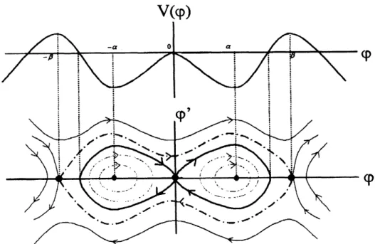
Figure 1: Phase portrait and Potential: the

case

of$P<0,$ $Q<0,$$V_{+}(\beta)>0$.

a thick solid line:

a

homoclinic orbit,

a

dotted line:

a

periodic orbit,

a

dash-dotted

line: a heteroclinic orbit, a thin solid line:

a

blow-up orbit

where, $\alpha$ and $\beta$

are

the positive solutions of$f_{+}(x)=0$ under the assumption

$0<c^{4}< \frac{4}{27}a^{6}$

.

(4.3)

The fixed points are classified

as

(0,0) : center, $(\alpha, 0)$ : saddle, $(\beta, 0)$ : center.

Similarly, for the

area

$\varphi<0$, the fixed points of the system

$\{\begin{array}{l}\varphi’=\eta,(4.4)\eta’=-b^{2}\varphi(1-a^{2}\varphi^{2}-c^{2}\varphi^{3})(=b^{2}\varphi f_{-}(\varphi))\end{array}$

are

given

as

$(\varphi, \eta)=(-\beta, 0),$ $(-\alpha, 0)$ $(0<\alpha<\beta)$,

and the fixed points

are

classffied

as

$(-\beta, 0)$ : center, $(-\alpha, 0)$ : saddle.

Thus, the similar unification argument to the

one

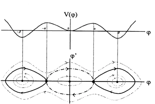
in the previous section realizes

the phase portrait in Figure 4 with its potential which shows the existence of both

bright and dark solitons. Tha fact that bright and dark solitons in Theorem 2.1(2) satisfy Fact 1 is easily found.

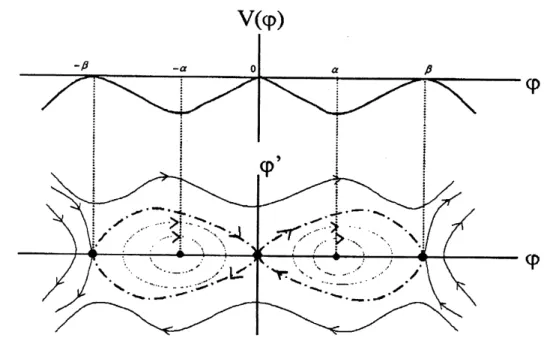
Figure 2: Phase portrait and Potential: the case of $P<0,$ $Q<0,$ $V_{+}(\beta)=0$

.

a dotted line:

a

periodic orbit,

a

dash-dotted line:

a

heteroclinic orbit,

a

thin solid

line:

a

blow-up orbit

The potential is derived from (4.2)

as

$V_{+}(\varphi):=b^{2}\varphi^{2}v_{+}(\varphi)$, where $v_{+}( \varphi)=\frac{1}{2}-\frac{a^{2}}{4}\varphi^{2}+\frac{c^{2}}{5}\varphi^{3}$

.

For realizingthe orbitsofthe bright solitons,

one

mustimpose the condition $V_{+}(\alpha)>$

$V_{+}(\beta)$. However, this condition for the potential

energy

$V_{+}$ is automatically fulfilled

without imposing any smallness assumption on thecoefficient $\epsilon$ except the condition

(4.3). In fact, $V_{+}’(\varphi)=-b^{2}\varphi f_{+}(\varphi)>0$ for the interval _{$\alpha<\varphi<\beta$} implies

$V_{+}(\alpha)>$

$V_{+}(\beta)$.

5

The

_case

$P<0,$ $Q>0$

In this case, there

are no

soliton for both $c=0$ and $c\neq 0$

.

The equation (2.3)

can

be given

as

$\varphi’’=b^{2}\varphi(1+\hat{a}^{2}|\varphi|^{2}+c^{2}|\varphi|^{3})$,

for $\hat{a}^{2}$ $:= \frac{Q}{\Omega}$, hence,

the second derivative is always positive for all $\varphi>0$, which

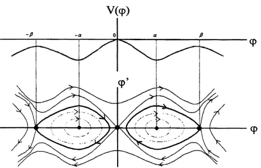
Figure 3: Phase portrait and Potential: the

case

of$P<0,$ $Q<0,$ $V_{+}(\beta)<0$.

a thick solid line: a homoclinic orbit, a dotted line: a periodic orbit, a thin solid

line:

a

blow-up orbit

6

The

case

$P>0,$ $Q>0$

The equation (2.3) for this

case

becomes

$\varphi’’=-\hat{b}^{2}\varphi(1+\hat{a}^{2}|\varphi|^{2}+c^{2}|\varphi|^{3})$,

which implies that the second derivative is always negative for all $\varphi>0$. For $c=0$,

it

can

be easily

seen

that there is only

one

fixed point $(0,0)$ for the above equation.

Moreover, the fixed point (0,0) is not

a

saddle point, but a center point. Hence,

there is no soliton for the

case

$c=0$.

For $c\neq 0$, the phase portrait is exactly the

same as

the

case

$c=0$

.

This is

because the zero point of the polynomial $1+a^{2}\varphi^{2}+c^{2}\varphi^{3}$ locates in _$\varphi<0$, while,

the zero point of the polynomial $1+a^{2}\varphi^{2}-c^{2}\varphi^{3}$ is in $\varphi>0$, hence, the formula

$1+a^{2}|\varphi|^{2}+c^{2}|\varphi|^{3}$ does not have

zero

points. Hence, there is the only

one

fixed point $(0,0)$, i.e., a _center. Thus, we can conclude that there is no _{soliton for both}

cases

$c=0$ and $c\neq 0$.

7

Conclusion

We have considered the one-dimensional cubic-quartic nonlinear Schr\"odinger

equa-tion (CQNLS). Solitons of the standing

wave

solutions have been investigated by phase portrait analysis. For two

cases

$(P<0$ and $Q<0)$ and $(P>0$ and $Q<0)$,

it is observed that there

are

both bright and dark solitons simultaneously when the

Figure 4: Phase portrait _{and Potential: the}

_case

_{of $P>0,$$Q<0$}

_.

a thick solid line:

a

homoclinic orbit, a dotted line: a periodic orbit,

a

dash-dotted

line:

a

heteroclinic orbit,

a

thin solid line: a blow-up orbit

References

[Agrawa197] _{Agrawal, G. P., Fiber-Optic Communication System, 2nd ed.,}

John Wiley&Son, Inc., New York, 1997.

[Nohara04] Nohara, B. T. ‘The stability ofthe governing equation of

enve-lope surface created by nearly bichromatic

waves

propagating

on an

elastic plate’, The Fourth World Congress

_of

Nonlinear

Analysts Orlando, FL, USA, June 30-July 7, 2004.

[Nohara05a] Nohara, B. T., ‘Governing equations of envelope surface

cre-ated by nearly bichromatic

waves

propagating

on an

elastic

plate and their stability’, Japan Joumal

_of

Industrial and

Ap-plied Mathematics 22(1), 2005, 89-111.

[Nohara05b] Nohara, B. T. and Arimoto, A., ‘The stability of the

govem-ing equation ofenvelope surface created by nearly bichromatic

waves

propagatingon an elastic plate’, NonlinearAnalysis

pa-per number: NA4234, 2005.

[Nohara06] _{Nohara, B. T. and Arimoto,} A., ‘On the Approximation

For-mula of Single Soliton Solution of Nonlinear Schr”odinger

Equation with High Order _{Perturbed Terms’ PDEs and}

Nohara07] Nohara B. T. and Arimoto A., (2007), Analysis of the

sin-gle soliton solution for the nonlinear Schr\"odinger equations

with higher perturbed terms, RIMS Kokyuroku, 171-180, in Japanese.

[Watanabe85] S. Watanabe, Introduction to Soliton Physics, Baifukan (1985),in Japanese.

[Zakharov72] Zakharov, V.E. and Shabat, A. B., ‘Exact theory of

two-dimensional selffocusing and one-dimensional self modulation

of

waves

in nonlinear media’, Soviet Physics, J.E. T.P. 34, 1972, 62-69.