AN INDEFINITE SUPERLINEAR ELLIPTIC EQUATION WITH A NONLINEAR BOUNDARY CONDITION OF SUBLINEAR TYPE (Shapes and other properties of solutions of PDEs)
21
0
0
全文
(2) 69. the standard. boundary point. non‐negative. weak solutions of. lemma. (P_{ $\lambda$}). (as. [14]). in. can. not be. applied directly. to nontrivial. .. The purpose of this paper is to study existence, non‐existence, and multiplicity of positive solutions of (P_{ $\lambda$}) , as well as their asymptotic properties as the parameter $\lambda$ ap‐ O. It is. proaches we. shall. see. (P_{ $\lambda$}). condition is known to Neumann we. paper. boundary focus. that (P_{ $\lambda$}) has no positive solution if a\geq 0 More precisely, positive solution only if \displaystyle \int_{ $\Omega$}a<0 (cf. Proposition 2.3). This be necessary for the existence of positive solutions of problems with. promptly. that. on. seen. has. .. a. conditions at least since the work of Bandle‐Pozio‐Tesei. the. case. where. a. changes sign.. In view of the condition. belongs. In this. 1<q<2<p we note that if a changes sign then (P_{ $\lambda$}) the class of concave‐convex type problems with nonlinear boundary conditions. reference on concave‐convex type problems is the work of Ambrosetti‐Brezis‐. to. The main. Cerami. [3].. [2],. ,. which deals with. \left\{ begin{ar y}{l -\triangleu=$\lambda$|u^{q-2}u+| ^{p-2}u&\mathrm{i}\mathrm{n} $\Omega$,\ u=0&\mathrm{o}\mathrm{n}\parti l$\Omega$, \end{ar y}\right.. (1.2). 1<q<2<p Under the condition (1.1) the authors proved a global multiplicity result, namely, the existence of some $\Lambda$>0 such that (1.2) has at least two positive solutions for $\lambda$\in(0, $\Lambda$) at least one positive solution for $\lambda$= $\Lambda$ and no positive solution for $\lambda$> $\Lambda$ In addition, they analysed the asymptotic behavior of the solutions as $\lambda$\rightarrow 0^{+} Tarfulea [21] considered a similar problem with an indefinite weight and a Neumann boundary condition, namely, where. .. ,. ,. .. .. \left\{ begin{ar y}{l -\triangleu=$\lambda$|u^{q-2}u+a(x)|u^{p-2}u&\mathrm{i}\mathrm{n} $\Omega$,\ \frac{\parti lu}{\parti l\mathrm{n}=0&\mathrm{o}\mathrm{n}\parti l$\Omega$, \end{ar y}\right. a\in C(\overline{ $\Omega$}). (1.3). He proved that \displaystyle \int_{ $\Omega$}a<0 is a necessary and sufficient condition for the positive solution of (1.3). Making use of the sub‐supersolutions technique, he has also shown the existence of $\Lambda$>0 such that problem (1.3) has at least one positive solution for $\lambda$< $\Lambda$ which converges to 0 in L^{\infty}( $\Omega$) as $\lambda$\rightarrow 0^{+} and no positive solution for $\lambda$> $\Lambda$ Garcia‐Azorero, Peral, and Rossi [10] have considered the problem where. existence of. .. a. ,. .. of. \left{\begin{ar y}{l -\triangleu+=|u^{p-2}u&\mathrm{i}\ athrm{n}$\Omega$,\ frac{\partil\mathrm{u}\partil\mathrm{n}=$\lambda$|u^{q-2}u&\mathrm{o}\mathrm{n}\partil$\Omega$. \end{ar y}\right.. (1.4). approach, they proved that if 1<q<2<p and p<2^{*} when $\Lambda$_{0}>0 such that (1.4) has infinitely many nontrivial weak solutions for 0< $\lambda$< $\Lambda$ Moreover, they have also proved that if 1<q<2 and p=2^{*} when N>2 then there exists $\Lambda$_{1}>0 such that (1.4) has at least two positive solutions for $\lambda$<$\Lambda$_{1} at least one positive solution for $\lambda$=$\Lambda$_{1} and no positive solution for $\lambda$>$\Lambda$_{1}.. By. means. a. variational. N>2 , then there exists .. ,. ,. When. shall prove. global multiplicity result in the style of However, doing so we shall encounter some particu‐ lar difficulties. First of all, the obtention of a first solution by the sub‐supersolution method seems difficult since the existence of a strict supersolution of (P_{ $\lambda$}) for $\lambda$>0 small is not evident at all. As a matter of fact, in [21] the author shows that this is a rather delicate issue. Another diffculty in this case is related to the variational structure: note that unlike in problems with Dirichlet boundary conditions, the left‐hand side of (P_{ $\lambda$}) lacks coercivity, since the term \displaystyle \int_{ $\Omega$}|\nabla u|^{2} does not correspond to \Vert u\Vert^{2} in X This sort of problems has been considered in [15, 16] for other kinds of nonlinearities and we shall use a similar approach here to prove existence results for (P_{ $\lambda$}) This approach is based on the Nehari manifold method, which is known to be useful when dealing with elliptic problems with powerlike a. changes sign. we. Ambrosetti‐Brezis‐Cerami result.. a. in. .. ..
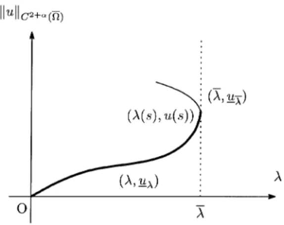
(3) 70. nonlinearities and the. Brown and Wu. sign‐changing weights.. [5]. used this method to deal with. problem. \left\{ begin{aray}{l -\triangleu=$\lambda$m(x)|u^{q-2}u+a(x)|u^{p-2}u&\mathrm{i}\mathrm{n} $\Omega$,\ u=0&\mathrm{o}\mathrm{n}\partial$\Omega$, \end{aray}\right.. (1.5). where m, a are smooth functions which are positive somewhere in $\Omega$ We refer also to Brown [4] for a combination of sublinear and linear terms and to Wu [23] for a problem with .. a. nonlinear. boundary. condition.. \displaystyle \int_{ $\Omega$}a<0. Whenever. we. set. c^{*}=(\displayst le\frac{|\parti l$\Omega$|}{-\int_{$\Omega$} )^{\frac{1}\mathrm{p}-q. We also set. \displaystyle \mathrm{A}=\sup { $\lambda$>0:(P_{ $\lambda$}) Let. recall that. us. (respect. unstable) of the linearized. In. addition,. u. positive solution. eigenvalue problem. at. positive solution}.. a. of. u. (P_{ $\lambda$}). <0 ), where. is said to be. $\gamma$_{1}( $\lambda$, u). asymptotically stable eigenvalue. is the smallest. namely,. u,. \left{\begin{ar y}{l -\triangle$\phi$=(p-1)a(xu^{p-2}$\phi$+ \gam a\phi$&\mathrm{i}\mathrm{n}$\Omega$,\ frac{\partil$\phi$}{\partil\mathrm{n}=$\lambda$(q-1)u^{q-2}$\phi$+ \gam a\phi$&\mathrm{o}\mathrm{n}\partil$\Omega$. \end{ar y}\right.. is said. We state. a. $\gamma$_{1}( $\lambda$, u)>0 (respect.. if. has. (1.6). weakly. now our. stable if. (1.7). $\gamma$_{1}( $\lambda$, u)\geq 0.. main result:. Theorem 1.1.. (1) (P_{ $\lambda$}). has. positive solution for $\lambda$>0 sufficiently small if. a. \displaystyle\int_{$\Omega$}a<0 Conversely, if (P_{ $\lambda$}). (2). Assume. (1.8).. has. a. Then the. (a) 0<\overline{ $\lambda$}\leq\infty. and. positive solution for. (P_{ $\lambda$}). has. some. (1.8). $\lambda$>0 then. is. satisfied.. assertions hold:. following. positive solution following properties: any. (1.8). .. minimal positive solution \underline{u}_{$\lambda$} for $\lambda$\in(0, \overline{ $\lambda$}) , i.e. in St. Furthermore \underline{u}_{ $\lambda$} has the. a. of (P_{ $\lambda$}) satisfies \underline{u}_{ $\lambda$}\leq u. u. (i) $\lambda$\mapsto\underline{u}_{ $\lambda$}(x) is strictly increasing in (0, \overline{ $\lambda$}) (ii) \underline{u}_{$\lambda$} is asymptotically stable for every $\lambda$\in(0, \overline{ $\lambda$}) (iii) $\lambda$\mapsto\underline{u}_{ $\lambda$} is C^{\infty} from (0,\overline{ $\lambda$}) to C^{2+ $\alpha$}(\overline{ $\Omega$}) (iv) \underline{u}_{ $\lambda$}\rightar ow 0 and $\lambda$^{-\frac{1}{p-q} \underline{u}_{ $\lambda$}\rightar ow c^{*} in C^{2+ $\alpha$}(\overline{ $\Omega$}) as $\lambda$\rightarrow 0^{+}. .. .. .. (b). Assume. (1.1). If \overline{ $\lambda$}<\infty. then. (P_{ $\lambda$}). Moreover the solution set around. has. $\epsilon$>0 , and. satisfies. u(s)=\underline{u}_{\overline{ $\lambda$}}+s$\phi$_{1}+z(s) smallest branch. branch. eigenvalue ,. positive solution \underline{u}_{\overline{$\lambda$} for $\lambda$= A.. of a C^{\infty} ‐curve ( $\lambda$(s), u(s))\in parametrized by s\in(- $\epsilon$, $\epsilon$) for. consists. which is. ,. ( $\lambda$(0), u(0) =(\overline{ $\lambda$}, \underline{u}_{\overline{ $\lambda$}}) $\lambda$'(0)=0, $\lambda$''(0)<0 ,. where. a. .. ,. ,. is unstable.. ,. and. associated to the. $\phi$_{1} positive eigenfunction of (1.7), and z(0)=z'(0)=0 Finally, the s\in(- $\epsilon$, 0) is asymptotically stable, whereas the ,. is. $\gam a$_{1}(\overline{$\lambda$},\underline{u}_{\overline{$\lambda$}). ( $\lambda$(s), u(s)) ( $\lambda$(s), u(s)) s\in(0, $\epsilon$) ,. minimal. (\overline{$\lambda$},\underline{u}_{\overline{$\lambda$}). \mathbb{R}\times C^{2+ $\alpha$}(\overline{ $\Omega$}) of positive solutions, some. a. lower upper.
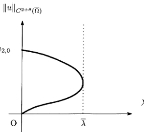
(4) 71. (c). Assume p<2^{*}. if N>2. ( $\lambda$, u)=(0,0). around. Then the set. .. of positive solutions of (P_{ $\lambda$}) for $\lambda$>0 of \{( $\lambda$, \underline{u}_{ $\lambda$})\}.. in \mathbb{R}\times X consists. (d) Bifurcation from zero of (P_{ $\lambda$}) never occurs at any $\lambda$>0 i.e. sequence ($\lambda$_{n}, u_{n}) of positive solutions of (P_{ $\lambda$}) such that u_{n}\rightarrow 0. there is. ,. in. C(\overline{ $\Omega$}). no. and. $\lambda$_{n}\rightarrow$\lambda$^{*}>0.. (e) (P_{ $\lambda$}). has at most. one. weakly. stable positive solution.. Remark 1.2.. (1). (1.8) and (1.1), by ( $\lambda$(s), u(s)) s\in(- $\epsilon$, 0) in. Under conditions. infer that. ,. solutions. In. (2). Under. (1.1). particular,. the. the minimal. $\gamma$_{1}(\overline{ $\lambda$},\underline{u}_{\overline{ $\lambda$} )=0. (3). of \underline{u}_{ $\lambda$} [ 1 Theorem 20.3], we 1.1(2)(b) represents minimal positive mapping $\lambda$\mapsto\underline{u}_{ $\lambda$} is continuous from (0, \overline{ $\lambda$}] into C(\overline{ $\Omega$}) ,. (0,0). is. left‐continuity. ,. .. positive solution \underline{u}_{\overline{$\lambda$} obtained for $\lambda$= A satisfies. In accordance with Theorem. solutions at. the. Theorem. 1.1, if \overline{ $\lambda$}<\infty then the in Figure 1.. set of. in addition. bifurcating positive. represented. \Vert u\Vert_{C^{2+ $\alpha$} (\overline{ $\Omega$}). FIGURE 1. A smooth Theorem 1.3.. Assume that. a. positive solution. changes sign. and. curve. (1.8). is. when. \overline{ $\lambda$}<\infty.. satisfied.. Then the. following. assertions hold:. (1) If a>0 (2). on. \partial $\Omega$ then. Assume in addition u_{2, $\lambda$}. p<\displaystyle \frac{2N}{N-2}. satisfying \underline{u}_{ $\lambda$}<u_{2, $\lambda$}. every any. \overline{ $\lambda$}<\infty.. $\lambda$\in(0, \overline{ $\lambda$}). $\theta$\in(0, $\alpha$). if N>2. \overline{$\Omega$} for. .. Then. (P_{ $\lambda$}). $\lambda$\in(0, \overline{ $\lambda$}). (P_{ $\lambda$}). in. second. positive solution. every. and there exists. as. n\rightarrow\infty ,. Remark 1.4. In accordance with Theorems 1.1 and. depicted. a. .. \left\{ begin{ar y}{l -\triangleu=a(x)u^{p-1}&in $\Omega$,\ \frac{\partilu}{\partil\mathrm{n}=0&on\partil$\Omega$. \end{ar y}\right.. is. has. Moreover, u_{2, $\lambda$} is unstable such that $\lambda$_{n}\rightarrow 0^{+} u_{2,$\lambda$_{n}}\rightarrow u_{2,0} in C^{2+ $\theta$}(\overline{ $\Omega$}) where u_{2,0} is a positive solution of. in. Figure. 2.. 1.3,. a. for for. (1.9) possible positive solutions. set of.
(5) 72. \Vert u\Vert_{C^{2+ $\theta$} (\overline{ $\Omega$}). $\lambda$. FIGURE 2. A. possible bifurcation diagram. for. (P_{ $\lambda$}). when. changes sign.. The outline of this article is the. following:. in Section 2. we. \displaystyle \int_{ $\Omega$}a<0. and. a. show that nontrivial. non‐. positive (P_{ $\lambda$}) positive solutions of (P_{ $\lambda$}) discuss existence of bifurcating positive use variational techniques to discuss multiplicity of positive solutions and their asymptotic profiles as $\lambda$\rightarrow 0^{+} Finally, in Section 5 we discuss existence of a unbounded subcontinuum of positive solutions of (P_{ $\lambda$}) in $\lambda$\in \mathbb{R} The details of the proofs of Theorems 1.1 and 1.3 negative. solutions of. necessary condition for the (1.8) In Section 3 we carry out a bifurcation analysis to solutions to the region $\lambda$>0 at (0,0) In Section 4 we. are. on. existence of. .. St and that. is. a. .. .. .. appear in. [18].. 2. POSITIVITY AND A NECESSARY CONDITION. positivity on \partial $\Omega$ of nontrivial non‐negative weak the boundary point lemma is difficult Introduction, (P_{ $\lambda$}) to apply directly to (P_{ $\lambda$}) since 0<q-1<1 However, by making good use of a comparison principle for a class of nonlinear boundary value problems of concave type, we are able to show that nontrivial non‐negative weak solutions of (P_{ $\lambda$}) with $\lambda$>0 are positive on the We. begin. solutions of. this section .. showing. the. As mentioned in the. .. whole of St:. Proposition 2.1. Assume (1.1). is strictly positive on \overline{ $\Omega$}.. Then any nontrivial. non‐negative weak solution of (P_{ $\lambda$}). Proof. First of all, we note that under (1.1) any nontrivial non‐negative weak solution belongs to X\cap C^{ $\theta$}(\overline{ $\Omega$}) for some $\theta$\in(0,1) cf. Rossi [20, Theorem 2.2]. We consider the following boundary value problem of concave type ,. \left{\begin{ar y}{l -\triangleu=-a_{0}u^p-1}&\mathrm{i}\ athrm{n}$\Omega$,\ frac{\partilu}{\partil\mathrm{n}=$\lambda$u^{q-1}&\mathrm{o}\mathrm{n}\partil$\Omega$, \end{ar y}\right. where a^{-}=a^{+}-a , and a_{0}=\displaystyle \sup_{ $\Omega$}a^{-} for $\lambda$>0 satisfies. A nontrivial non‐negative weak solution u_{ $\lambda$} of. \displaystyle\int_{$\Omega$}\nablau_{$\lambda$}\nablaw+a_{0}\int_{$\Omega$}u_{$\lambda$}^{p-1}w-$\lambda$\int_{\partial$\Omega$}u_{$\lambda$}^{q-1}w\geq0,. (P_{ $\lambda$}).
(6) 73. for every w\in X such that w\geq 0. On the other. .. hand,. we. consider the. following eigenvalue. problem:. \left{bgin{ary}l -\triangle$\phi=$\sgma\phi$&\mathr{i}\mathr{n}$\Omega$,\ frac{\prtial$\phi}{ artil\mathr{n}=$\lambd\phi$&\mathr{o}\mathr{n}\partil$\Omega$. \end{ary}\ight.. (2.1). see that for any $\lambda$>0 this problem has a smallest eigenvalue $\sigma$_{1} which negative. So, using a positive eigenfunction $\phi$_{1} associated to $\sigma$_{1} we deduce that if $\epsilon$ sufficiently small then $\epsilon \phi$_{1} satisfies. It is easy to. ,. ,. is. is. \displaystyle \int_{ $\Omega$}\nabla( $\epsilon \phi$_{1})\nabla w+a_{0}\int_{ $\Omega$}( $\epsilon \phi$_{1})^{p-1}w- $\lambda$\int_{\partial $\Omega$}( $\epsilon \phi$_{1})^{q-1}w\leq 0,. for every w\in X such that w\geq O. By the comparison principle [16, infer that $\epsilon \phi$_{1}\leq u_{ $\lambda$} on \overline{$\Omega$} In particular, we have 0< $\epsilon \phi$_{1}\leq u_{ $\lambda$} on \partial $\Omega$.. Proposition A.1],. we. \square. .. positivity property, the assumption a\in C^{ $\alpha$}(\overline{ $\Omega$}) 0< $\alpha$<1, (1.1), any nontrivial non‐negative weak solution u of (P_{ $\lambda$}) to for some belongs C^{2+ $\theta$}(\overline{ $\Omega$}) $\theta$\in(0,1) by elliptic regularity. Proposition 2.1 will be needed in a combination argument of bifurcation and variational techniques, since our purpose in this paper is to discuss the existence of a classical solution of (P_{ $\lambda$}) which is positive in the Remark 2.2. Thanks to the allows. ,. to prove that under. us. ,. closure 9.. for. We prove $\lambda$>0.. now. that. (1.8). is. a. necessary condition for. (P_{ $\lambda$}). to have. positive solution. a. some. Proposition Proof.. Let. u. If (P_{ $\lambda$}). 2.3.. be. Since u^{1-p}\in X ,. a. has. a. positive solution for. positive solution of (P_{ $\lambda$}) Then .. we. $\lambda$>0 then. some. (1.8). is. satisfied.. have. \displaystyle \int_{ $\Omega$}\nabla u\nabla w-\int_{ $\Omega$}au^{p-1}w- $\lambda$\int_{\partial $\Omega$}u^{q-1}w=0, \foral w\in X. we. deduce that. \displaystyle \int_{ $\Omega$}a=\int_{ $\Omega$}\nabla u\nabla(u^{1-p})- $\lambda$\int_{\partial $\Omega$}u^{q-1}\frac{1}{u^{p-1} =(1-p)\int_{ $\Omega$}u^{-p}|\nabla u|^{2}- $\lambda$\int_{\partial $\Omega$}u^{-(p-q)}<0,. as. desired.. Remark 2.4.. By. Proposition 2.1, under (1.1) non‐negative weak solutions of (P_{ $\lambda$}). virtue of. holds for nontrivial. 3. A. zero. \Vert u_{n}\Vert\rightarrow 0 if We. and. use now a. solution of. (P_{ $\lambda$}). (1.1). If ($\lambda$_{n}, u_{n}). only if. 3.2.. 2.3. are. shall discuss bifurcation from the. for. weak solutions. a. similar. of (P_{ $\lambda$}). bifurcation. technique. proof):. with. ($\lambda$_{n}). bounded then. which. corresponds. to. to show the existence of at least. To this. (P_{ $\lambda$}). end,. we. after the. consider. change of. \left{\begin{ar y}{l -\trianglew=$\lambd$\frac{p-2} \mathr {q}aw^{p-1}&\mathr {i}\mathr {n}$\Omega$,\ frac{\prtialw}{\partiln}=$\lambd$\frac{p-2} qw^{-1}&\mathr {o}\mathr {n}\partil$\Omega$. \end{ar y}\right. Proposition. Proposition. \Vert u_{n}\Vert_{C(\overline{ $\Omega$})}\rightar ow 0.. for $\lambda$>0 close to O.. following problem,. prove that. BIFURCATION ANALYSIS. Throughout this section, we assume (1.8). As we solution, the following result will be useful (see [17]. Lemma 3.1. Assume. we can. \square. one positive positive solutions of the. variable. w=$\lambda$^{-\frac{1}{p-q}}u :. (3.1).
(7) 74. (1) If (3.1). C(\overline{ $\Omega$}). has. and. a. c. of positive. sequence. is. (2) Conversely, (3.1). solutions. ($\lambda$_{n}, w_{n}). such that. constant then c=c^{*} , where c^{*} is. positive. a. $\lambda$_{n}\rightarrow 0^{+},. w_{n}\rightarrow c in. given by (1.6).. has for| $\lambda$|. sufficiently small a secondary bifurcation branch ( $\lambda$, w( $\lambda$)) (parametrized by $\lambda$ ) emanating from the trivial line \{(0, c) : c is a positive constant} at (0, c^{*}) and such that, for 0< $\theta$\leq $\alpha$ the mapping $\lambda$\mapsto w( $\lambda$)\in C^{2+ $\theta$}(\overline{ $\Omega$}) is continuous. Moreover, the set \{( $\lambda$, w)\} of positive solu‐ tions of (3.1) around ( $\lambda$, w)=(0, c^{*}) consists of the union. of positive. solutions. ,. { (0, c). Proof.. (1). is. a. for. $\delta$_{1}>0.. The. proof. is similar to the. one. of. Let w_{n} be positive solutions of formula we have. to the limit. We reduce dure:. (3.1). we use. \cup\{( $\lambda$, w( $\lambda$)): | $\lambda$|\leq$\delta$_{1}\}. positive constant, |c-c^{*}|\leq$\delta$_{1} }. some. Passing. (2). : c. to. [16, Proposition 5.3]:. (3.1). with. $\lambda$=\mathrm{A}_{n} where $\lambda$_{n}\rightarrow 0^{+} ,. .. the Green. By. \displaystyle \int_{ $\Omega$}aw_{n}^{p-1}+\int_{\partial $\Omega$}w_{n}^{q-1}=0. n\rightarrow\infty , we. as. a. deduce the desired conclusion.. bifurcation equation in \mathbb{R}^{2}. the usual. by. the. Lyapunov‐Schmidt. proce‐. orthogonal decomposition. L^{2}( $\Omega$)=\mathbb{R}\oplus V, where. V=\displaystyle \{v\in L^{2}( $\Omega$) : \int_{ $\Omega$}v=0\}. and the. projection. Q:L^{2}( $\Omega$)\rightarrow V given by ,. v=Qu=u-\displaystyle \frac{1}{| $\Omega$|}\int_{ $\Omega$}u. The. of. problem problems:. where. finding. a. positive solution of (3.1) reduces then. to the. following. \left\{ begin{ar y}{l -\trianglev+\frac{$\mu$}{|$\Omega$|}\int_{\parti l$\Omega$}(t+v)^{q-1}=$\mu$Q[a(t+v)^{p-1}]&\mathrm{i}\mathrm{n} $\Omega$,\ \frac{\parti lv}{\parti l\mathrm{n}=$\mu$(t+v)^{q-1}&\mathrm{o}\mathrm{n}\parti l$\Omega$, \end{ar y}\right.. (3.2). $\mu$(\displaystyle \int_{ $\Omega$}a(t+v)^{p-1}+\int_{\partial $\Omega$}(t+v)^{q-1})=0. (3.3). $\mu$= $\lambda$\displaystyle \frac{p-2}{p-q}, t=\displaystyle \frac{1}{| $\Omega$|}\int_{ $\Omega$}w. Hölder spaces,. we. ,. and v=w-t. .. To solve. ,. (3.2). in the framework of. set. Y=\displaystyle \{v\in C^{2+ $\theta$}(\overline{ $\Omega$}):\int_{ $\Omega$}v=0\}, Z=\displaystyle \{( $\phi$, $\psi$)\in C^{ $\theta$}(\overline{ $\Omega$})\times C^{1+ $\theta$}(\partial $\Omega$):\int_{ $\Omega$} $\phi$+\int_{\partial $\Omega$} $\psi$=0\}. Let c>0 be. a. constant and U\subset \mathbb{R}\times \mathbb{R}\mathrm{x}Y be. We consider the nonlinear. a. small. neighborhood. of. (0, c, 0). F( $\mu$, t, v)=(-\displaystyle \triangle v- $\mu$ Q[a(t+v)^{p-1}]+\frac{ $\mu$}{| $\Omega$|}\int_{\partial $\Omega$}(t+v)^{q-1}, \displaystyle\frac{\partialv}{\partial\mathrm{n} -$\mu$(t+v)^{q-1}) The Fréchet derivative. .. mapping F:U\rightarrow Z given by. F_{v} of F with respect. to. v. at. F_{v}(0, c, 0)v=(-\displaystyle \triangle v, \frac{\partial v}{\partial \mathrm{n} ). .. (0, c, 0). is. .. given by the formula.
(8) 75. F_{v}(0, c, 0) is a homeomorphism, the implicit function theorem implies that the F( $\mu$, t, v)=0 around (0, c, 0) consists of a unique C^{\infty} function v=v( $\mu$, t) in a neighborhood of ( $\mu$, t)=(0, c) and satisfying v(0, c)=0 Now, plugging v( $\mu$, t) in (3.3), we obtain the bifurcation equation Since. set. .. $\Phi$( $\mu$, t)=\displaystyle \int_{ $\Omega$}a(t+v( $\mu$, t) ^{p-1}+\int_{\partial $\Omega$}(t+v( $\mu$, t) ^{q-1}=0 $\Phi$(0, c^{*})=0 Differentiating. It is clear that. .. for. ,. ( $\mu$, t)\simeq(0, c). $\Phi$ with respect to t at. .. (0, c^{*}). get. we. $\Phi$_{t}(0, c^{*})=\displaystyle \int_{ $\Omega$}a(p-1)(c^{*}+v(0, c^{*}) ^{p-2}(1+v_{t}(0, c^{*}) +\displaystyle \int_{\partial $\Omega$}(q-1)(c^{*}+v(0, c^{*}) ^{q-2}(1+v_{t}(0, c^{*}) =(p-1)(c^{*})^{p-2}\displaystyle \int_{ $\Omega$}a(1+v_{t}(0, c^{*}) +(q-1)(c^{*})^{q-2}\int_{\partial $\Omega$}(1+v_{t}(0, c^{*} Differentiating. (3.2). now. v_{t}(0, c^{*})=0. have. with respect to t , and. Hence. .. plugging ( $\mu$, t)=(0, c^{*}) therein,. we. $\Phi$_{t}(0, c^{*})=(p-1)(c^{*})^{p-2}(\displaystyle \int_{ $\Omega$}a)+(q-1)(c^{*})^{q-2}|\partial $\Omega$|=|\partial $\Omega$|^{\frac{p-2}{p-q} (-\int_{ $\Omega$}a)^{\frac{2-\mathrm{q} {p-q} (q-p)<0. By. the. $\lambda$\displaystyle\frac{p-2}{p-q}. implicit function theorem, the function w( $\lambda$)=t( $\mu$)+v( $\mu$, t( $\mu$)) with. $\mu$=. satisfies the desired assertion. \square. By considering Proposition is. suficiently. the transform. Let 0< $\theta$\leq $\alpha$ and. 3.3.. small then. $\lambda$^{-\frac{1}{p-\mathrm{q} }u( $\lambda$)\rightar ow c^{*}. in. u( $\lambda$)= $\lambda$\displaystyle \frac{1}{p-q}w( $\lambda$) w( $\lambda$). as. $\lambda$\rightarrow 0^{+}. .. we. get the following result:. be. given by Proposition 3.2. If $\lambda$>0 positive solution of (P_{ $\lambda$}) which satisfies In particular, u( $\lambda$)\rightarrow 0 in C^{2+ $\theta$}(\overline{ $\Omega$}) as $\lambda$\rightarrow 0^{+}.. u( $\lambda$)= $\lambda$\displaystyle \frac{1}{p-q}w( $\lambda$). C^{2+ $\theta$}(\overline{ $\Omega$}). ,. is. a. 4. VARIATIONAL APPROACH. We associate to. (P_{ $\lambda$}). the C^{1} functional. I_{ $\lambda$}(u) :=\displaystyle \frac{1}{2}E(u)-\frac{1}{p}A(u)-\frac{ $\lambda$}{q}B(u) , u\in X, where. E(u)=\displaystyle \int_{ $\Omega$}|\nabla u|^{2}, A(u)=\displaystyle \int_{ $\Omega$}a(x)|u|^{p} Let. recall that. us. We denote The. X=H^{1}( $\Omega$). \mathrm{b}\mathrm{y}\rightar ow \mathrm{t}\mathrm{h}\mathrm{e}. following. is. equipped. ,. B(u)=\displaystyle \int_{\partial $\Omega$}|u|^{q}.. and. with the usual. norm. weak convergence in X. result will be used. repeatedly. \displaystyle \Vert u\Vert=[\int_{ $\Omega$}(|\nabla u|^{2}+u^{2})]^{\frac{1}{2}. in this section.. Lemma 4.1.. (1) If (u_{n}). is. a. sequence such that u_{n}\rightarrow u_{0} in X and. limsupn E(u_{n})\leq 0. constant and u_{n}\rightarrow u_{0} in X.. (2) Proof.. Assume. (1.8). If v\neq 0. and. A(v)\geq 0. ,. then. v. is not. a. constant.. then u_{0}\dot{u}a.
(9) 76. (1). Since u_{n}\rightarrow u_{0} in X and E is so that. weakly lower semicontinuous,. we. E(u_{0})\leq. have. \displaystyle \lim\inf_{n}E (un),. 0\leq E(u_{0})\leq Hence, E(u_{0})=0 Then X.. (2). If. which. E(u_{n})\leq. limninf. limnsup E(u_{n})\leq 0.. that u_{0} is a constant. Assume u_{n}\star u_{0} in X. E(u_{0})<\displaystyle \lim\sup_{n}E(u_{n})\leq 0 , which is a contradiction. Therefore u_{n}\rightarrow u_{0} in. v_{0}\neq 0. is. a. ,. implies. constant then. 0\displaystyle \leq A(v_{0})=|v_{0}|^{p}\int_{ $\Omega$}a<0. a. ,. contradiction. \square. (1.1). in addition to. Now, assume. p<\displaystyle \frac{2N}{N-2}. if N>2. .. (1.8),. and. we. assume. that. a. changes sign. Moreover, we positive solutions of (P_{ $\lambda$}). We shall prove the existence of two. for 0< $\lambda$< A and characterize their asymptotic profiles fibering maps associated to. the Nehari manifold and the. $\lambda$\rightarrow 0^{+}. as. I_{ $\lambda$}. Let. .. us. .. To this. introduce. end,. we use. some. useful. subsets of X :. E^{+}=\{u\in X : E(u)>0\},. A^{\pm}=\{u\in X:A(u)\gtrless 0\}, A_{0}=\{u\in X:A(u)=0\}, A_{0}^{\pm}=A^{\pm}\cup A_{0}, B^{+}=\{u\in X : B(u)>0\}. The Nehari manifold associated to. I_{ $\lambda$}. is. given by. N_{ $\lambda$} :=\{u\in X\backslash \{0\} : \langle I_{ $\lambda$}'(u), u\}=0\}=\{u\in X\backslash \{0\} : E(u)= $\Lambda$(u)+ $\lambda$ B(u)\}. We shall. use. the. splitting. N_{ $\lambda$}=N_{ $\lambda$}^{+}\cup N_{ $\lambda$}^{-}\cup N_{ $\lambda$}^{0}, where. N_{ $\lambda$}^{\pm}. :=\{u\in N_{ $\lambda$} : \{J_{ $\lambda$}'(u), u\}\gtrles 0\}=\{u\in N_{ $\lambda$} E(u)\displaystyle \les gtr $\lambda$\frac{p-q}{p-2}B(u)\} =\{u\in N_{ $\lambda$} E(u)\displaystyle \gtrles \frac{p-q}{2-q}A(u)\}, :. :. and. N_{ $\lambda$}^{0}=\{u\in N_{ $\lambda$} : \{J_{ $\lambda$}'(u), u\}=0\}. Note that any nontrivial weak solution of the implicit function theorem that restriction of. I_{ $\lambda$}. to this manifold is. analyse the structure of u\neq 0 in the following way: To. for. It is easy to. (P_{ $\lambda$}) belongs. N_{ $\lambda$}\backslash N_{ $\lambda$}^{0} a. is. critical. N_{ $\lambda$}^{\pm}. ,. we. a. to N_{ $\lambda$} Furthermore, it follows from C^{1} manifold and every critical point of the .. point of I_{ $\lambda$} (see for. consider the. fibering. instance maps. [6,. Theorem. corresponding. 2.3]). to. I_{ $\lambda$}. j_{u}(t):=I_{ $\lambda$}(tu)=\displaystyle \frac{t^{2} {2}E(u)-\frac{t^{p} {p}A(u)- $\lambda$\frac{t^{q} {q}B(u) , t>0.. see. that. j_{u}'(1)=0\lessgtr j_{u}''(1)\Leftrightarrow u\in N_{ $\lambda$}^{\pm}, and. more. generally,. j_{u}'(t)=0\lessgtr j_{u}''(t)\Leftrightarrow tu\in N_{ $\lambda$}^{\pm}. Having. this characterisation in. mind,. we. look for conditions under which. j_{u} has. point. Set. i_{u}(t) :=t^{-q}j_{u}(t)=\displaystyle \frac{t^{2-q} {2}E(u)-\frac{t^{p-q} {p}A(u)- $\lambda$ B(u) , t>0.. a. critical.
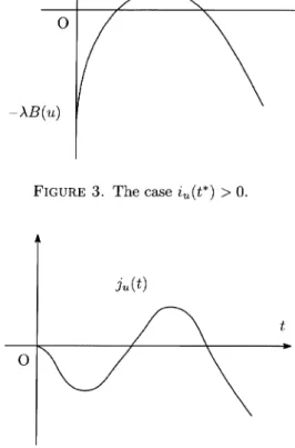
(10) 77. Let. u\in E^{+}\cap A^{+}\cap B^{+}. Then i_{u} has a global maximum i_{u}(t^{*}) at some t^{*}>0 , and i_{u}(t^{*})>0 , then j_{u} has a global maximum which is positive and. .. moreover, t^{*} is unique. If a local minimum which is. negative. Moreover, these. are. the. only. critical. points of j_{u}. .. We. i_{u}(t). FIGURE 3. The. FIGURE 4. A. shall require. if and. only. if. a. condition. only. on. of j_{u}. having. $\lambda$ that. a. global. i_{u}(t^{*})>0.. maximum and. provides i_{u}(t^{*})>0. .. F(u). local minimum.. Note that. t=t^{*}:=(\displaystyle \frac{p(2-q)E(u)}{2(p-q)A(u)})^{\frac{1}{p-2} if. i_{u}(t^{*})=\displaystyle\frac{p-2}{2(p-q)}(\frac{p(2-q)}{2(p-q)} ^{\frac{2-q}{p-2} \frac{E(u)^{\frac{p-q}{\mathrm{p}-2} {A(u)^{\frac{2-q}{p-2} -\frac{$\lambda$}{q}B(u)>0 0< $\lambda$\displaystyle \frac{p-2}{p-q}<C_{pq}\frac{E(u)}{B(u)^{\frac{p-2}{p-q}A(u)^{\frac{2-q}{p-q} }. where. a. i_{u}'(t)=\displaystyle \frac{2-q}{2}t^{1-q}E(u)-\frac{p-q}{p}t^{p-q-1}A(u)=0. Moreover. if and. case. case. C_{pq}=(\displaystyle \frac{q(p-2)}{2(p-q)} ^{\frac{p-2}{p-q} (\frac{p(2-q)}{2(p-q)} ^{\frac{2-q}{p-\mathrm{q}. for t>0 , i.e. F is. Note that. homogeneous of order. O.. (4.1). ,. F(u)=\displaystyle \frac{E(u)}{B(u)^{\mathrm{L}- p-\frac{2}{q}A(u)^{\frac{2-}{p-}A}q}. satisfies. F(tu)=.
(11) 78. We deduce then the existence of critical. points. Proposition. The. 4.2.. following result,. which. provides sufficient conditions for the. of j_{u} :. following. assertions hold:. (1) If either u\in E^{+}\cap A_{0}^{-}\cap B^{+} or u\in A^{-}\cap B^{+} then j_{u}(t) has a negative global minimum at some t_{1}>0, i.e. j_{u}'(t_{1})=0<j_{u}''(t_{1}) and j_{u}(t)>j_{u}(t_{1}) for t\neq t_{1} Moreover, t_{1} is the unique critical point of j_{u} and j_{u}(t)\rightarrow\infty as t\rightarrow\infty. ,. .. (2) If u\in E^{+}\cap A^{+}\cap B_{0} then j_{u}(t) has a positive global maximum at some t_{2}>0, i.e. j_{u}'(t_{2})=0>j_{u}''(t_{2}) and j_{u}(t)<j_{u}(t_{2}) for t\neq t_{1} Moreover, t_{2} is the unique critical point of j_{u} and j_{u}(t)\rightarrow-\infty as t\rightarrow\infty. .. (3). Assume. (1.8). If. we. set. $\lambda$^{\frac{p-2}{0^{\mathrm{p}-q} }=\displaystyle \inf\{E(u):u\in E^{+}\cap A^{+}\cap B^{+}, C_{pq}^{-1}B(u)^{\frac{p-2}{p-q}A(u)^{\frac{2-\mathrm{q} {p-q} }=1\}. (4.2). ,. then $\lambda$_{0}> O. Moreover, for any 0< $\lambda$<$\lambda$_{0} and u\in E^{+}\cap A^{+}\cap B^{+} the map j_{u} has a negative local minimum at t_{1}>0 and a positive global maximum at t_{2}>t_{1}.. Furthermore, t_{1}, t_{2} Figure 4).. the. are. Proof. Assertions (1) and (2) (3). First, we show E^{+}\cap A^{+}\cap B^{+} satisfying. assertion. are. in. (u_{n}) is L^{p}( $\Omega$). X. From. bounded in X then. L^{q}(\partial $\Omega$) u_{n}\in A^{+} we. and. and. we. t\rightarrow\infty. (see. .. may. deduce that. as. ,. and. ,. j_{u}(t)\rightarrow-\infty. straightforward from the definition of j_{u} We prove now $\lambda$_{0}> O. Assume $\lambda$_{0}=0 so that we can choose u_{n}\in. C_{pq}^{-1}B(u_{n})^{4\mathrm{i}_{\frac{-2}{-q} }\mathrm{p}A(u_{n})^{\frac{2-q}{p-q} =1.. assume. It follows from Lemma. .. of j_{u}. that. E(u_{n})\rightarrow 0 If. critical points. only. u_{0}\in A_{0}^{+}. .. that u_{n}\rightarrow u_{0} for 4.1(1) that u_{0} is. In. addition,. we. some a. u_{0}\in X and. u_{n}\rightarrow u_{0}. constant and u_{n}\rightarrow u_{0} in. have. C_{pq}^{-1}B(u_{0})^{\frac{p-2}{p-q}A(u_{0})^{\frac{2-\mathrm{q} {p-q} }=1, 4.1(2) we get a contradiction. \Vert u_{n}\Vert\rightarrow\infty Set v_{n}=\displaystyle \frac{u}{\Vert u_{n}\Vert} so that \Vert v_{n}\Vert=1 assume that v_{n}\rightarrow v_{0} and v_{n}\rightarrow v_{0} in L^{p}( $\Omega$) Since E(v_{n})\rightarrow 0 and v_{n}\in A^{+} v_{n}\rightarrow v_{0} in X, v_{0} is a constant, and v_{0}\in A_{0}^{+} In particular, \Vert v_{0}\Vert=1 i.e. v_{0}\not\equiv 0 so. that. u_{0}\not\equiv 0. Let. us. .. From Lemma. assume. that. now. .. provides again. a. ,. .. have. Lemma. contradiction.. for any u\in E^{+}\cap A^{+}\cap B^{+}. Finally,. we. ,. .. 4.1. We may. .. ,. .. we. have. $\lambda$^{\frac{p-2}{0^{p-q} \displaystyle\leqC_{pq}\frac{E(u)}{B(u)^{\frac{p-2}{\mathrm{p}-q}A(u)^{\frac{2-q}{p-q} . Thus, if 0< $\lambda$<$\lambda$_{0}. then. (3).. i_{u}(t^{*})>0. from. (4.1).. This. completes. the. proof. of assertion \square. Proposition. (1) N_{ $\lambda$}^{0} (2) N_{ $\lambda$}^{\pm}. is. 4.3.. We. have, for 0< $\lambda$<$\lambda$_{0} :. empty. non‐empty.. are. Proof.. (1). From i.e.. Proposition. N_{ $\lambda$}^{0}. is empty.. 4.2 it follows that there is. no. t>0 such that. j_{u}'(t)=j_{\mathrm{u}}''(t)=0,.
(12) 79. (2). Consider the. Under. following eigenvalue problem. \left{\begin{ar y}{l -\triangle$\varphi$= \lambd$a(x)$\varphi$&\mathr {i}\mathr {n}$\Omega$,\ frac{\prtial$\vrphi$}{\partil\mathr {n}=0&\mathr {o}\mathr {n}\partil$\Omega$. \end{ar y}\ight.. (1.8). it is known that this. problem has a unique positive principal eigenvalue positive principal eigenfunction $\varphi$_{N} From $\varphi$_{N}>0 on \partial $\Omega$ and the fact that $\varphi$_{N} is not a constant, we deduce that $\varphi$_{N}\in E^{+}\cap A^{+}\cap B^{+} Since 0< $\lambda$<$\lambda$_{0}, Proposition 4.2(3) provides the desired conclusion. $\lambda$_{N} with. a. .. .. \square. The. following. Lemma 4.4. Let. result. provides. 0< $\lambda$<$\lambda$_{0}. Then,. .. (1) N_{ $\lambda$}^{+} is bounded in X. (2) I_{ $\lambda$}(u)<0 for any u\in N_{ $\lambda$}^{+}. properties of. some. have the. we. and. moreover. N_{ $\lambda$}^{+}. :. following. t>1. two assertions:. if j_{u}'(t)>0.. Proof.. (1). (\mathrm{u}_{n})\subset N_{ $\lambda$}^{+}. Assume we. assume. may. A(v)\rightarrow A(v_{0})). .. and. \Vert u_{n}\Vert\rightarrow\infty B(v_{n}). Set. .. that v_{n}\rightarrow v_{0}, Since. u_{n}\in N_{ $\lambda$}^{+}. ,. is. v_{n}=\displaystyle \frac{u_{n} {\Vert u_{n}\Vert}. bounded,. \Vert v_{n}\Vert=1 so L^{p}( $\Omega$) (implying. It follows that. .. and v_{n}\rightarrow v_{0} in. ,. that. we see. E(v_{n})< $\lambda$\displaystyle \frac{p-q}{p-2}B(v_{n})\Vert u_{n}\Vert^{q-2}, \displaystyle \lim\sup_{n}E(v_{n})\leq 0. and thus in X. Lemma. .. Consequently, \Vert v_{0}\Vert=1. .. u_{n}\in N_{ $\lambda$}. ,. ,. 4.1(1) yields. and v_{0} is. a. that v_{0} is. non‐zero. a. constant and v_{n}\rightarrow v_{0}. constant.. However,. since. that. we see. 0\leq E(u_{n})=A(u_{n})+ $\lambda$ B(u_{n}). ,. and it follows that. 0\leq A(v_{n})+ $\lambda$ B(v_{n})\Vert u_{n}\Vert^{q-p}. Passing. to the limit. as. n\rightarrow\infty , we. contradiction. Therefore. (2). Let. u\in N_{ $\lambda$}^{+}. .. N_{ $\lambda$}^{+}. deduce. 0\leq A(v_{0}). .. Lemma. 4.1(2). leads. to. us. a. is bounded in X.. Then. 0\displaystyle \leq E(u)< $\lambda$\frac{p-q}{p-2}B(u). ,. so that B(u)>0 First we assume that u is not a constant. In this case E(u)>0 If A(u)>0 then Proposition 4.2(3) tells us that I_{ $\lambda$}(u)<0 and t>1 if j_{u}'(t)>0 On the other hand, if A(u)\leq 0 then u\in E^{+}\cap A_{0}^{-}\cap B^{+} So Proposition 4.2(1) gives the .. .. .. .. same so. conclusion. Assume. that u\in A^{-}\cap B^{+}. .. now. that. is. u. a. constant. In this. Proposition 4.2(1) again yields. case. A(u)=|u|^{p}\displaystyle \int_{ $\Omega$}a<0,. the desired conclusion.. \square Next. we. prove that. \displaystyle \inf_{N_{ $\lambda$}^{+} I_{ $\lambda$}. is achieved. by. some. u_{1, $\lambda$}>0. for. $\lambda$\in(0, $\lambda$_{0}). ,. which. implies the estimate \overline{ $\lambda$}\geq$\lambda$_{0} Furthermore, we can show that u_{1, $\lambda$} positive solution of (P_{ $\lambda$}) for $\lambda$>0 suffciently small.. is in fact the minimal. Proposition. I_{$\lambda$}(u_{1,$\lambda$})=\displaystyle\min_{N_{$\lambda$}^{+} I_{$\lambda$}. .. 4.5. For any. particular, u_{1, $\lambda$}. is. a. 0< $\lambda$<$\lambda$_{0} there ,. positive solution of (P_{ $\lambda$}). .. exists u_{1, $\lambda$} such that. .. In.
(13) 80. Proof.. 0< $\lambda$<$\lambda$_{0} We consider. Let. .. a. minimizing. (u_{n})\subset N_{ $\lambda$}^{+}. sequence. i.e.. ,. I_{ $\lambda$}(u_{n})\displaystyle \rightar ow\inf_{N_{ $\lambda$}^{+} I_{ $\lambda$}<0. Since. (u_{n}). is bounded in X ,. we. may. assume. L^{p}( $\Omega$). that u_{n}\rightarrow u_{0}, u_{n}\rightarrow u_{0} in. and. L^{q}(\partial $\Omega$). .. It follows that. I_{ $\lambda$}(u_{0})\displaystyle \leq\lim_{n}\inf I_{ $\lambda$}(u_{n})=\inf_{N_{ $\lambda$}^{+} I_{ $\lambda$}(u)<0, so. that. u_{0}\not\equiv 0. We claim that u_{n}\rightarrow u_{0} in X. .. We have two. .. possibilities:. B(u_{0})=0 then u_{0}=0 on \partial $\Omega$, which yields a contradiction. Hence B(u_{0})>0 In this case, so that u_{0}=0 in $\Omega$ we have A(u_{0})=|u_{0}|^{p}\displaystyle \int_{ $\Omega$}a<0 so that u_{0}\in A^{-}\cap B^{+} Proposition 4.2(1) implies If u_{0} is. \bullet. constant, then. a. 0=E(u_{0})\displaystyle \leq $\lambda$\frac{p-q}{p-2}B(u_{0}). .. If. .. ,. .. ,. t_{1}u_{0}\in N_{ $\lambda$}^{+}. that. and. j_{u_{0}}. has. a. global. minimum at t_{1}. If. .. \mathrm{n}_{0}. then. (4.3). I_{ $\lambda$}(t_{1}u_{0})=j_{u_{0} (t_{1})\displaystyle \leq j_{u_{\mathrm{O} }(1)<\lim_{n}\dot{\mathrm{m} \mathrm{f}j_{u_{n} (1)= limninf I_{ $\lambda$}(u_{n})=\displaystyle \inf_{N_{ $\lambda$}^{+} I_{ $\lambda$)} which is. contradiction since. a. If u_{0} is not or. a. constant then. u_{0}\in E^{+}\cap A^{+}\cap B^{+}. can. argue. t_{1}u_{0}\in N_{ $\lambda$}^{+}. E(u_{0})>0. .. and. Therefore u_{n}\rightarrow u_{0}.. B(u_{0})>0. .. u_{0}\in E^{+}\cap A_{0}^{-}\cap B^{+}. So either. In the first case, j_{u_{\mathrm{O} } has a global minimum point t_{1} and we in the previous case. In the second case, since 0< $\lambda$<$\lambda$_{0} , Proposition. as. .. t_{1}u_{0}\in N_{ $\lambda$}^{+}. yields that have again 4.2. for. t_{1}> O. Assume u_{n}\neq\neq u_{0}. some. I_{ $\lambda$}(t_{1}u_{0})=j_{u_{0}}(t_{1})\leq j_{u_{0}}(1)<. If 1<t_{1} then. .. limninf j_{u_{n}}(1)= limninf I_{ $\lambda$}(u_{n})=\displaystyle \inf_{N_{ $\lambda$}^{+} I_{ $\lambda$}. If t_{1}<1 then j_{u_{n}}'(t_{1})<0 for every n , a contradiction. Therefore u_{n}\rightarrow u_{0}.. so. that. Now, since u_{n}\rightarrow u_{0} we have j_{u_{0}}'(1)=0\leq j_{u_{0}}''(1) Proposition 4.3(1). Thus u_{0}\in N_{ $\lambda$}^{+} and. .. But. j_{u_{0}}''(1)=0. is. (4.4). ,. j_{u_{0}}'(t_{1})<\displaystyle \lim\inf j_{u_{n}}'(t_{1})\leq 0. we. ,. which is. impossible by \square. I_{$\lambda$}(u_{0})=\displaystyle\inf_{N_{$\lambda$}^{+} I_{$\lambda$}.. Remark 4.6. From. Next. \displaystyle \inf_{N_{ $\lambda$}^{-} I_{ $\lambda$}. we. for. Proposition. obtain. a. $\lambda$\in(0, $\lambda$_{0}). Lemma 4.7. Let. .. 4.5. we. derive. \overline{ $\lambda$}\geq$\lambda$_{0}.. second nontrivial non‐negative weak solution of (P_{ $\lambda$}) , which achieves The following result provides some properties of N_{ $\lambda$}^{-} :. 0< $\lambda$<$\lambda$_{0}. .. Then. we. have. I_{ $\lambda$}(u)>0 for. j_{u}'(t)>0.. any. u\in N_{ $\lambda$}^{-}. .. Moreover t<1. if. Proof If u\in N_{ $\lambda$}^{-} then A(u)>0 and u is not a constant from Lemma 4.1(2). It follows immediately that E(u)>0 If B(u)>0 then, by Proposition 4.2(3), we have that I_{ $\lambda$}(u)>0 \square and t<1 if j_{u}'(t)>0 If B(u)=0 then Proposition 4.2(2) provides the same conclusion. .. .. Proposition. 4.8. For any. particular, u_{2, $\lambda$}. Proof.. Since. is. a. ,. ,. $\lambda$\in(0, $\lambda$_{0}). ,. there exists u_{2, $\lambda$} such that. positive solution of (P_{ $\lambda$}). I_{ $\lambda$}(u)>0. for. u\in N_{ $\lambda$}^{-}. ,. we can. I_{$\lambda$}(u_{2,$\lambda$})=\displaystyle\min_{N_{$\lambda$}^{-} I_{$\lambda$}. .. choose. u_{n}\in N_{ $\lambda$}^{-}. I_{ $\lambda$}(u_{n})\rightar ow N^{\frac{\mathrm{f} { $\lambda$} \mathrm{i}\mathrm{n}I_{ $\lambda$}(u)\geq 0.. such that. .. In.
(14) 81. We claim that. (u_{n}). Since u_{n}\in N_{ $\lambda$}. we. ,. is bounded in X. I_{ $\lambda$}(u_{n})\leq C.. exists C>0 such that. Indeed, there. .. deduce. (\displaystyle \frac{1}{2}-\frac{1}{p})E(u_{n})- $\lambda$(\frac{1}{q}-\frac{1}{p})B(u_{n})=I_{ $\lambda$}(u_{n})\leq C. \Vert u_{n}\Vert\rightarrow\infty and set v_{n}=\displaystyle \frac{u_{n} {\Vert u_{n}| } so that \Vert v_{n}\Vert=1 v_{n}\rightarrow v_{0} in L^{p}( $\Omega$) and L^{q}(\partial $\Omega$) Then, from. Assume and. We may. .. ,. that v_{n}\rightarrow v_{0},. assume. .. (\displaystyle \frac{1}{2}-\frac{1}{p})E(v_{n})\leq $\lambda$(\frac{1}{q}-\frac{1}{p})B(v_{n})\Vert u_{n}\Vert^{q-2}+\frac{C}{\Vert u_{n}\Vert^{2} , we. \displaystyle \lim\sup_{n}E(v_{n})\leq 0. infer that. in X , which. Lemma. .. implies \Vert v_{0}\Vert=1 However, .. 4.1(1) yields u_{n}\in N_{ $\lambda$}^{-}. since. that v_{0} is ,. E(v_{n})\displaystyle \Vert u_{n}\Vert^{2-p}<\frac{p-q}{2-q}A(v_{n}) to the limit n\rightarrow\infty ,. Passing. get. we. (u_{n}). Hence. L^{q}(\partial $\Omega$). 0\leq A(v_{0}). which is. constant, and v_{n}\rightarrow v_{0}. .. .. .. implies that. u_{0} is not. a. .. ,. 0=j_{u_{\mathrm{O}}}'(t_{2})<\displaystyle \lim\inf_{n}j_{u}' ..(t2), ,. we. limninf \displaystyle \frac{p-q}{2-q}A(u_{n})=\frac{p-q}{2-q}A(u_{0}). we. deduce. .. by Lemma 4.1(2), so that E(u_{0})> O. Since u_{0}\in that there exists t_{2}>0 such that t_{2}u_{0}\in N_{ $\lambda$}^{-} Moreover, since u_{n}\neq\neq u_{0} We deduce that j_{ $\tau \iota$_{n}}'(t_{2})>0 for n large. constant. E^{+}\cap A^{+} Proposition 4.2 tells. enough. Since u_{n}\in N_{ $\lambda$}^{-}. 4.1(2). L^{p}( $\Omega$) and. Lemma. contradictory by. is bounded. We may then assume that u_{n}\rightarrow u_{0} , and u_{n}\rightarrow u_{0} in We claim that u_{n}\rightarrow u_{0} in X Assume u_{n}\neq u_{0} Then, since u_{n}\in N_{ $\lambda$}^{-} ,. 0\displaystyle \leq E(u_{0})<\lim\inf E(u_{n})\leq This. ,. a. observe that. we. us. .. .. t_{2}<1 from Lemma 4.7. Then,. have. observe that. we. I_{ $\lambda$}(t_{2}u_{0})=j_{u_{0} (t_{2})<\displaystyle \lim_{\mathrm{n} \inf j_{u_{n} (t_{2})\leq\lim\inf j_{u_{n} (1)=\lim\inf I_{ $\lambda$}(u_{n})=N^{\frac{\mathrm{f} { $\lambda$} \mathrm{i}\mathrm{n}I_{ $\lambda$}. This is. a. contradiction, which implies that. Now. verify. we. that. u_{0}\neq 0. .. u_{n}\rightarrow u_{0} and. Assume u_{0}=0. .. I_{ $\lambda$}(u_{n})\rightarrow I_{ $\lambda$}(u_{0})= $\gamma$.. Then,. u_{n}\in N_{ $\lambda$}. since. E(v_{n})\Vert u_{n}\Vert^{2-q}=A(v_{n})\Vert u_{n}\Vert^{p-q}+ $\lambda$ B(v_{n}) where. v_{n}=\displaystyle \frac{u_{n} {\Vert \mathrm{u}_{n}\Vert}. We may. .. to the limit. Passing hand, we. as. again. assume. 0= $\lambda$ B(v_{0}). ,. so. have. we. ,. that v_{n}\rightarrow v_{0} and v_{n}\rightarrow v_{0} in. obtain. n\rightarrow\infty , we. ,. that v_{0}=0. L^{q}(\partial $\Omega$). on. \partial $\Omega$. .. and. L^{p}( $\Omega$). .. On the other. observe that. 0<I_{ $\lambda$}(u_{n})=\displaystyle \frac{1}{2}E(u_{n})-\frac{1}{p}A(u_{n})-\frac{ $\lambda$}{q}B(u_{n}) Since u_{n}\in N_{ $\lambda$} ,. we. .. deduce. (\displaystyle \frac{1}{q}-\frac{1}{2})E(v_{n})\leq(\frac{1}{q}-\frac{1}{p})A(v_{n})\Vert u_{n}\Vert^{p-2}. From the. assumption u_{n}\rightarrow 0. get that v_{0} is v_{0}=0 on \partial $\Omega$. in X , it follows that. ,. \displaystyle \lim\sup E(v_{n})\leq 0 By .. Lemma. constant, and v_{n}\rightarrow v_{0} in X so that 1 v_{0}\Vert=1 Since v_{0} is This is a contradiction, as desired. we have v_{0}=0 in $\Omega$. a. .. ,. 4.1(1). we. constant and. .. Finally, since u_{n}\rightarrow u_{0} in X we have j_{u_{0}}'(1)=0\geq j_{u_{0}}''(1) But by Proposition 4.3(1). Thus u_{0}\in N_{ $\lambda$}^{-} and .. j_{u0}''(1)=0 is impossible. I_{$\lambda$}(u_{0})=N^{\frac{\mathrm{f}{$\lambda$}\mathrm{i}\mathrm{n}I_{$\lambda$}.. We discuss. a. now. the. \square. asymptotic profiles of u_{1, $\lambda$}, u_{2, $\lambda$} as $\lambda$\rightarrow 0^{+} The following lemma positive solutions in N_{ $\lambda$}^{+} as $\lambda$\rightarrow 0^{+} :. is concerned with the behavior of. ..
(15) 82. Proposition. If. 4.9.. u_{ $\lambda$} is. positive solution of (P_{ $\lambda$}) such that u_{ $\lambda$}\in N_{ $\lambda$}^{+} for $\lambda$>0 sufi‐ as $\lambda$\rightarrow 0^{+} Moreover there holds $\lambda$^{-\frac{1}{p-q} u_{ $\lambda$}\rightar ow c^{*} in C^{2+ $\theta$}(\overline{ $\Omega$}). a. ciently small then u_{ $\lambda$}\rightarrow 0 in X for any $\theta$\in(0, $\alpha$) as $\lambda$\rightarrow 0^{+}.. Proof.. First. \Vert u_{ $\lambda$}\Vert\rightar ow\infty. we. .. show that u_{ $\lambda$} remains bounded in X as $\lambda$\rightarrow 0^{+} Indeed, assume that We may then assume that for some v_{0}\in X we have v_{ $\lambda$}\rightarrow v_{0} .. and set. v_{$\lambda$}=\displaystyle\frac{u_{$\lambda$}{\Vertu_{$\lambda$}\Vert} L^{p}( $\Omega$). in X , and v_{ $\lambda$}\rightarrow v_{0} in. .. L^{q}(\partial $\Omega$). and. .. Since u_{ $\lambda$}\in N_{ $\lambda$} ,. we. have. E(v_{ $\lambda$})\Vert u_{ $\lambda$}\Vert^{2-p}=A(v_{ $\lambda$})+ $\lambda$ B(v_{ $\lambda$})\Vert u_{ $\lambda$}\Vert^{q-p}. to the limit. Passing. as. $\lambda$\rightarrow 0^{+}. obtain. we. ,. A(v_{0})=0. .. u_{ $\lambda$}\in N_{ $\lambda$}^{+}. From. have. we. E(v_{ $\lambda$})< $\lambda$\displaystyle \frac{p-q}{p-2}B(v_{ $\lambda$})\Vert u_{ $\lambda$}\Vert^{q-2}, so. that. X,. so. \displaystyle \lim\sup_{ $\lambda$}E(v_{ $\lambda$})\leq 0 By Lemma 4.1(1) we infer that v_{0} is a constant and v_{ $\lambda$}\rightarrow v_{0} in \Vert v_{0}\Vert=1 i.e. v_{0}\neq 0 This is contradictory with Lemma 4.1(2), and therefore .. that. .. ,. stays bounded in X. u_{ $\lambda$}. Hence. $\lambda$\rightarrow 0^{+}. we. Since. .. may. $\lambda$\rightarrow 0^{+}.. as. assume. u_{ $\lambda$}\in N_{ $\lambda$}^{+}. we. ,. that u_{ $\lambda$}\rightarrow u_{0} in X and u_{ $\lambda$}\rightarrow u_{0} in. E(u_{ $\lambda$})< $\lambda$\displaystyle \frac{p-q}{p-2}B(u_{ $\lambda$}) to the limit. Passing is. as. $\lambda$\rightarrow 0^{+}. ,. constant and u_{ $\lambda$}\rightarrow u_{0} in X. a. implies A(u_{0})=0. ,. so. we .. get. \displaystyle \lim\sup_{ $\lambda$}E(u_{ $\lambda$})\leq 0. Since u_{ $\lambda$}\in N_{ $\lambda$} ,. we. we. obtain the. that u_{0}=0 from Lemma. $\psi$_{ $\lambda$}\rightar ow$\psi$_{0}. in. that. L^{p}( $\Omega$). Lemma. 4.1(2) provides. 4.1(2).. that u_{0}. Therefore u_{ $\lambda$}\rightarrow 0 in X. .. .. .. as. We. ,. \Vert w_{ $\lambda$}\Vert\rightar ow\infty and set $\psi$_{ $\lambda$}=\displaystyle \frac{w_{ $\lambda$} {\Vert w_{ $\lambda$}\Vert} L^{q}(\partial $\Omega$) It follows that. and. as. .. E(w_{ $\lambda$})<\displaystyle \frac{p-q}{p-2} $\lambda$\frac{p-2}{p-q}B(w_{ $\lambda$}) us assume. .. asymptotic profile of u_{ $\lambda$} as $\lambda$\rightarrow 0^{+} Let w_{ $\lambda$}=$\lambda$^{-\frac{1}{p-q} u_{ $\lambda$} as $\lambda$\rightarrow 0^{+} Indeed, since u_{ $\lambda$}\in N_{ $\lambda$}^{+} we have. claim that w_{ $\lambda$} remains bounded in X. Let. L^{q}(\partial $\Omega$). have. $\lambda$\rightarrow 0^{+}.. Now. and. .. E(u_{ $\lambda$})=A(u_{ $\lambda$})+ $\lambda$ B(u_{ $\lambda$}) which. L^{p}( $\Omega$). observe that. .. .. We may. assume. that. $\psi$_{ $\lambda$}\rightar ow$\psi$_{0}. and. .. E($\psi$_{ $\lambda$})<\displaystyle \frac{p-q}{p-2} $\lambda$\frac{p-2}{p-q}B($\psi$_{ $\lambda$})\Vert w_{ $\lambda$}\Vert^{q-2}, so. that. in X. \displaystyle \lim\sup_{ $\lambda$}E($\psi$_{ $\lambda$})\leq 0 By .. On the other. .. Lemma. hand, from u_{ $\lambda$}\in N_{ $\lambda$}. 4.1(1). we. infer that. 0\leq A(u_{ $\lambda$})+ $\lambda$ B(u_{ $\lambda$}) so. $\psi$_{0}. is. a. constant and. $\psi$_{ $\lambda$}\rightar ow$\psi$_{0}. it follows that ,. that. -B($\psi$_{ $\lambda$})\Vert w_{ $\lambda$}\Vert^{q-p}\leq A($\psi$_{ $\lambda$}). .. stays bounded in X. $\lambda$\rightarrow 0^{+} we get 0\leq A($\psi$_{0}) which contradicts Lemma 4.1(2). Hence w_{ $\lambda$} as $\lambda$\rightarrow 0^{+} and we may assume that w_{ $\lambda$}\rightarrow w_{0} in X and w_{ $\lambda$}\rightarrow w_{0} in. L^{p}( $\Omega$). It follows that. Taking. w_{0} is. the limit. and. a. as. L^{q}(\partial $\Omega$). .. ,. \displaystyle \lim\sup_{ $\lambda$}E(w_{ $\lambda$})\leq 0. ,. and. by. Lemma. constant and w_{ $\lambda$}\rightarrow w_{0} in X.. It remains to show that w_{0}=c^{*}. .. 4.1(1). we. get that. We note that w_{ $\lambda$} satisfies. \displaystyle \int_{ $\Omega$}\nabla w_{ $\lambda$}\nabla w- $\lambda$\frac{p-2}{p-q}\int_{ $\Omega$}aw_{ $\lambda$}^{p-1}w- $\lambda$\frac{p-2}{p-q}\int_{\partial $\Omega$}w_{ $\lambda$}^{q-1}w=0, \foral w\in X. ,. (4.5).
(16) 83. since u_{ $\lambda$} is. a. weak solution of. (P_{ $\lambda$}) Taking .. w=1 ,. that. we see. \displaystyle\int_{$\Omega$}aw_{$\lambda$}^{p-1}+\int_{\partial$\Omega$}w_{$\lambda$}^{q-1}=0. Passing. to the limit. w=\displaystyle \frac{1}{w_{ $\lambda$}^{q-1}. in. (4.5). $\lambda$\rightarrow 0^{+}. as. we. ,. that either. we see. w_{0}=0. or. w_{0}=c^{*}. However, taking. .. obtain. 0>-(q-1)\displaystyle \int_{ $\Omega$}w_{ $\lambda$}^{-q}|\nabla w_{ $\lambda$}|^{2}= $\lambda$\frac{p-2}{\mathrm{p}-q}(\int_{ $\Omega$}aw_{ $\lambda$}^{p-q}+|\partial $\Omega$|). ,. that. so. |\displaystyle\partial$\Omega$|<-\int_{$\Omega$}aw_{$\lambda$}^{p-q}. It is clear then that. By. a. w_{0}\neq 0 i.e. w_{0}=c^{*} and consequently we obtain bootstrap argument, we get the desired conclusion.. standard We turn. now. that solutions in Lemma 4.10.. ,. to the. N_{ $\lambda$}^{-}. If u_{ $\lambda$}. is. Proof. Assume by. asymptotic behavior of u_{2, $\lambda$}. bounded away from. are. a. \Vert u_{ $\lambda$}\Vert\geq C for. small then. ,. and. $\lambda$\rightarrow 0^{+}. as. .. in X.. \square. We shall prove. initially. $\lambda$\rightarrow 0^{+} :. positive solution of (P_{ $\lambda$}) such that u_{ $\lambda$}\in N_{ $\lambda$}^{-} for $\lambda$>0 suficiently constant C>0 as $\lambda$\rightarrow 0^{+}.. some. (u_{n}) \Vert u_{n}\Vert\rightarrow 0 Then,. contradiction that. $\lambda$_{n}\rightarrow 0^{+}, u_{n}\in N_{$\lambda$_{n} ^{-}. zero as. $\lambda$^{-\frac{1}{p-q} u_{ $\lambda$}\rightar ow c^{*}. .. is. a. sequence of. since. u_{n}\in N_{$\lambda$_{n} ^{-}. ,. positive solutions of (P_{$\lambda$_{n} ) with deduce. we. E(v_{n})<\displaystyle \frac{p-q}{2-q}A(v_{n})\Vert u_{n}\Vert^{p-2}, where. v_{n}=\displaystyle \frac{u_{n} {\Vert u_{n}\Vert}. .. We may. assume. that v_{n}\rightarrow v_{0} in X and v_{n}\rightarrow v_{0} in. \displaystyle \lim\sup E(v_{n})\leq 0 By Lemma 4.1(1) we get that v_{0} is a so that \Vert v_{0}\Vert=1 On the other hand, we see that A(v_{n})>0 then 0\leq A(v_{0}) which is a contradiction with Lemma 4.1(2). that. .. L^{p}( $\Omega$). It follows. .. constant and v_{n}\rightarrow v_{0} in. .. ,. since. u_{n}\in N_{$\lambda$_{n} ^{-}. \square. ,. We prove Lemma 4.11.. Proof. By. now. that u_{2, $\lambda$} is bounded in X. There exists. Lemma 4.10. we. a. as. $\lambda$\rightarrow 0^{+} :. constant C>0 such that. know that. X,. We obtain. .. \Vert u_{2, $\lambda$}\Vert\geq C^{-1}. for. C^{-1}\leq\Vert u_{2, $\lambda$}\Vert\leq C some. C>0. as. as. $\lambda$\rightarrow 0^{+}.. $\lambda$\rightarrow 0^{+}. .. We show. that u_{2, $\lambda$} is bounded in X as $\lambda$\rightarrow 0^{+} First, we show that there exists a constant C_{1}>0 such that I_{ $\lambda$}(u_{2, $\lambda$})\leq C_{1} for every $\lambda$\in(0, $\lambda$_{0}) To this end, we consider the following. now. .. .. eigenvalue problem. with the Dirichlet. boundary condition.. \left{\begin{ar y}{l -\triangle$\varphi$= \lambda$ (x)$\varphi$&\mathrm{i}\mathrm{n}$\Omega$,\ $\varphi$=0&\mathrm{o}\mathrm{n}\partil$\Omega$. \end{ar y}\right.. We denote. by $\varphi$_{D} a positive eigenfunction associated $\lambda$_{D} Multiplying (4.6) by $\varphi$_{D}^{\mathrm{p}-1} we see that $\varphi$_{D}\in A^{+} .. .. with the. Thus. j_{$\varphi$_{D} (t)=\displaystyle \frac{t^{2} {2}E($\varphi$_{D})-\frac{t^{p} {p}A($\varphi$_{D}) so. that. neither. has. j_{$\varphi$_{D} j_{$\varphi$_{D}. t_{2}$\varphi$_{D}\in N_{ $\lambda$}^{-}. nor ,. we. (4.6) positive principal eigenvalue. $\varphi$_{D}\in E^{+}\cap A^{+}\cap B_{0}. and. ,. global maximum at some t_{2}>0 which implies t_{2}$\varphi$_{D}\in N_{ $\lambda$}^{-} Moreover, t_{2}$\varphi$_{D} depend on $\lambda$\in(0, $\lambda$_{0}) Let C_{1}=j_{$\varphi$_{D}}(t_{2})=I_{ $\lambda$}(t_{2}$\varphi$_{D})> O. Since. a. ,. .. deduce that. I_{ $\lambda$}(u_{2, $\lambda$})\leq C_{1}.. ..
(17) 84. Assume. \Vert u_{2, $\lambda$}\Vert\rightar ow\infty as $\lambda$\rightarrow 0^{+} and L^{p}( $\Omega$) and L^{q}(\partial $\Omega$) Since. that. now. v_{ $\lambda$}\rightarrow v_{0} and v_{ $\lambda$}\rightarrow v_{0} in. set. v_{$\lambda$}=\displaystyle\frac{u_{2,$\lambda$}{\Vertu_{2$\lambda$}\Vert}. A(v_{ $\lambda$})>. it follows that. will. u_{2, $\lambda$}\in N_{ $\lambda$}. ,. we. to the limit. Passing. O.. that the condition. see. We may. assume. that. .. 0\displaystyle \leq E(u_{2, $\lambda$})<\frac{p-q}{2-q}A(u_{2, $\lambda$}) we. .. I_{ $\lambda$}(u_{2, $\lambda$})\leq C_{1}. ,. $\lambda$\rightarrow 0^{+}. as. leads. us. to. we. ,. a. get. A(v_{0})\geq. contradiction.. O. However, Indeed, since. deduce. (\displaystyle \frac{1}{2}-\frac{1}{p})E(u_{2, $\lambda$})-(\frac{1}{q}-\frac{1}{p}) $\lambda$ B(u_{2, $\lambda$})=I_{ $\lambda$}(u_{2, $\lambda$})\leq C_{1}.. Hence. (\displaystyle \frac{1}{2}-\frac{1}{p})E(v_{ $\lambda$})\leq(\frac{1}{q}-\frac{1}{p}) $\lambda$ B(v_{ $\lambda$})\Vert u_{2, $\lambda$}\Vert^{q-2}+C_{1}\Vert u_{2, $\lambda$}\Vert^{-2}.. Letting $\lambda$\rightarrow 0^{+}. obtain. we. constant and v_{ $\lambda$}\rightarrow v_{0} in X. proof. is. .. complete.. now. We establish. \displaystyle \lim\sup_{ $\lambda$}E(v_{ $\lambda$})\leq 0 and by Lemma 4.1 we infer that v_{0} In particular, \Vert v_{0}\Vert=1 which contradicts Lemma 4.1(2). ,. ,. is. a. The \square. now. (up. to. a. subsequence). the. precise limiting behavior of u_{2, $\lambda$} :. Proposition 4.12. There exists a sequence $\lambda$_{n}\rightarrow 0^{+} such for any $\theta$\in(0, $\alpha$) where u_{2,0} is a positive solution of (1.9).. that u_{2,$\lambda$_{n}}\rightarrow u_{2,0} in. C^{2+ $\theta$}(\overline{ $\Omega$}). ,. Proof. Since u_{2, $\lambda$} stays bounded in X as $\lambda$\rightarrow 0^{+} , up to a subsequence, we have u_{2, $\lambda$}\rightarrow u_{2,0}, and u_{2, $\lambda$}\rightarrow u_{2,0} in L^{p}( $\Omega$) and L^{q}(\partial $\Omega$) as $\lambda$\rightarrow 0^{+} Since u_{2, $\lambda$} is a weak solution of (P_{ $\lambda$}) , we have .. Letting $\lambda$\rightarrow 0^{+}. i.e. u_{2,0} is. \displaystyle \int_{ $\Omega$}\nabla u_{2, $\lambda$}\nabla w-\int_{ $\Omega$}au_{2, $\lambda$}^{p-1}w- $\lambda$\int_{\partial $\Omega$}u_{2, $\lambda$}^{q-1}w=0, \foral w\in X. ,. we. get. \displaystyle \int_{ $\Omega$}\nabla u_{2,0}\nabla w-\int_{ $\Omega$}au_{2,0}^{p-1}w=0, \foral w\in X, a. non‐negative. weak solution of. (1.9).. E(u_{2, $\lambda$})<\displaystyle \frac{p-q}{2-q}A(u_{2, $\lambda$}) we. deduce that. \displaystyle \lim\sup_{ $\lambda$}E(u_{2, $\lambda$})\leq 0 By .. If. u_{2,0}\equiv 0 then,. and. Lemma. from. A(u_{2,0})=0,. 4.1(1). we. infer that u_{0} is. a. constant and. u_{2, $\lambda$}\rightarrow u_{2,0}=0 in X which contradicts Lemma 4.11. Finally, since u_{2,0}\in C^{2+ $\alpha$}(\overline{ $\Omega$}) and u_{2,0}>0 in 9 by the weak maximum principle and the boundary point lemma, we infer that u_{2,0} is a positive solution of (1.9). By a standard \square bootstrap argument, we obtain the desired conclusion. ,. ,. We shall consider. now. the Palais‐Smale condition for I_{ $\lambda$}. the Palais‐Smale condition if any sequence such that in X' has a convergent subsequence.. Proposition Proof.. Let. be. a. Palais‐Smale sequence for I_{ $\lambda$}. (I_{ $\lambda$}(u_{n})) In. particular,. we. (I_{ $\lambda$}(u_{n})). I_{ $\lambda$} satisfies the Palais‐Smale condition for. 4.13.. (u_{n}). .. is bounded. and. .. Let. us. recall that. is bounded and. I_{ $\lambda$} satisfies. I_{ $\lambda$}'(u_{n})\rightarrow 0. any $\lambda$>0... Then. I_{ $\lambda$}'(u_{n}) $\phi$=o(1)\Vert $\phi$\Vert. \forall $\phi$\in X.. have. (\displaystyle \frac{1}{2}-\frac{1}{p})E(u_{n})- $\lambda$(\frac{1}{q}-\frac{1}{p})B(u_{n})=I_{ $\lambda$}(u_{n})-\frac{1}{p}I_{ $\lambda$}'(u_{n})u_{n}\leq c+o(1)\Vert u_{n}\Vert. (4.7).
(18) 85. for. constant. some. c. .. \Vert u_{n}\Vert\rightarrow\infty and set v_{n}=\displaystyle \frac{u_{n} {\Vert u_{n}\Vert} L^{p}( $\Omega$) and L^{q}(\partial $\Omega$) From. Assume that. v_{n}\rightarrow v in X and v_{n}\rightarrow v in. .. Then. we. \displaystyle \int_{ $\Omega$}\nabla u_{n}\nabla $\phi$-a(x)|u_{n}|^{p-2}u_{n} $\phi$- $\lambda$\int_{\partial $\Omega$}|u_{n}|^{q-2}u_{n} $\phi$=o(1)\Vert $\phi$\Vert, \foral $\phi$\in X so. \displaystyle \int_{ $\Omega$}a(x)|v_{n}|^{p-2}v_{n} $\phi$\rightar ow 0 \foral $\phi$\in X. that. This we. (4.8). \Vert u_{n}\Vert^{p-1},. get, dividing it by. we. that. assume. may. .. equality implies. that. \displaystyle \int_{ $\Omega$}a(x)|v|^{p-2}v $\phi$=0 \foral $\phi$\in X.. a|v|^{p-2}v=0. a.e.. in $\Omega$. Hence av\equiv 0. .. .. Taking. now. $\phi$=v. in. obtain. (4.8),. \displaystyle \int_{ $\Omega$}\nabla v_{n}\nabla v- $\lambda$\Vert u_{n}\Vert^{q-2}\int_{\partial $\Omega$}|v_{n}|^{q-2}v_{n}v\rightar ow 0. \displaystyle\int_{$\Omega$}\nablav_{n}\nablav\rightar ow0. Thus. we get \displaystyle \int_{ $\Omega$}|\nabla v|^{2}= O. So v must be a constant. From av\equiv 0, Finally, from (4.7), dividing it by \Vert u_{n}\Vert^{2} we obtain E(v_{n})\rightarrow 0. Therefore, by Lemma 4.1, we have v_{n}\rightarrow 0 in X which contradicts \Vert v_{n}\Vert=1. So (u_{n}) must be bounded, and up to a subsequence, u_{n}\rightarrow u in X and u_{n}\rightarrow u in L^{p}( $\Omega$) and L^{q}(\partial $\Omega$) Taking $\phi$=u_{n}-u in (4.8) we get. and since v_{n}\rightarrow v in X ,. we. deduce that. v\equiv. O.. ,. .. consequently \Vert u_{n}\Vert^{2}\rightar ow\Vert u\Vert^{2}. and X.. \displaystyle\int_{$\Omega$}|\nablau_{n}|^{2}\rightar ow\int_{$\Omega$}|\nablau|^{2} .. By. the uniform. convexity of. X,. we. infer that u_{n}\rightarrow u in \square. multiplicity result for positive solutions of (P_{ $\lambda$}) for $\lambda$\in(0, \overline{ $\lambda$}) First all, by Proposition 4.5 or Proposition 4.8, we know that \overline{ $\lambda$}\geq$\lambda$_{0}> O. We proceed now as in [9] to obtain a solution by the variational form of the sub‐supersolution method. \mathrm{A} version of this method for a problem with Neumann boundary conditions has been proved in [11 Theorem 3]. We shall use a slightly different version of this result, namely: We prove. now a. .. of. ,. Theorem 4.14. Let such that. for. $\Omega$\times[-R, R] are. :. $\Omega$\times \mathbb{R}\rightarrow \mathbb{R} and. and. g:\partial $\Omega$\times \mathbb{R}\rightarrow \mathbb{R} be Carathéodory functions. M=M(R)>0 satisfying |f(x, s)|\leq M if (x, s)\in. |g(x, s)|\leq M if (x, s)\in\partial $\Omega$ \mathrm{x}[-R, R] If \underline{u}, \overline{u}\in H^{1}( $\Omega$)\cap L^{\infty}( $\Omega$)\cap L^{\infty}(\partial $\Omega$) supersolution of (P_{ $\lambda$}) respectively, and \underline{u}\leq\overline{u}a.e in $\Omega$ then .. weak subsolution and. a. (P_{ $\lambda$}). f. every R>0 there exists. has. solution. a. u. ,. .. satisfying. I_{ $\lambda$}(u)=\displaystyle \min\{I_{ $\lambda$}(v):v\in H^{1}( $\Omega$), \underline{u}\leq v\leq\overline{u} a.e. in $\Omega$\}. The a. proof of this result can fact, the functional I_{ $\lambda$}. matter of. M:=. Let. us. (2.1). we can. take. following. the. proof of [11,. { u\in H^{1}( $\Omega$):\underline{u}\leq u\leq\overline{u} prove that. $\mu$'\in( $\mu$, \overline{ $\lambda$}]. such that. a.e.. on. 3].. As. the set. in $\Omega$ }.. (P_{ $\mu$}) has two positive solutions. From the (P_{$\mu$'}) has a positive solution u_{$\mu$'} Now, we .. of the positive eigenfunction $\phi$_{1} associated to the smallest eigenvalue $\sigma$_{1} of to build up a suitable positive weak subsolution. We consider the smallest eigenvalue. good. use. \hat{$\sigma$}_{1} :=$\sigma$_{1}( $\mu$)<0 of (2.1) and the corresponding positive eigenfunction. $\epsilon$\hat{$\phi$}_{1}. Theorem. is not coercive but still bounded from below. pick 0< $\mu$< A and. definition of A make. be carried out. is. a. strict weak subsolution of. (P_{ $\mu$}). if $\epsilon$>0 is. sufficiently. small.. \hat{ $\phi$}_{1}=$\phi$_{1}( $\mu$) Moreover,. .. Then. we. can.
(19) 86. choose $\epsilon$>0 such that a. (P_{ $\mu$}). solution u_{0} of. $\epsilon$\hat{ $\phi$}_{1}\leq u_{$\mu$'}. .. Theorem 4.14 with. By. \underline{u}= $\epsilon$\hat{ $\phi$}_{1}. and. such that. I_{ $\mu$}(u_{0})=\displaystyle \min { I_{ $\mu$}(v):v\in H^{1}( $\Omega$). ,. $\epsilon$\hat{ $\phi$}_{1}\leq v\leq u_{$\mu$'}. a.e.. \mathrm{u}=u_{$\mu$'}. we. ,. obtain. in $\Omega$ }.. In particular, u_{0}>0 in \overline{$\Omega$} Moreover, by the strong maximum principle and the boundary point lemma we have $\epsilon$\hat{ $\phi$}_{1}<u_{0}<u_{$\mu$'} on 9. It follows that u_{0} is a local minimizer of I_{ $\mu$} with respect to the C^{1}(\overline{ $\Omega$}) topology. We may then argue as in [10, Lemma 6.4] to deduce that u_{0} is a local minimizer of I_{ $\mu$} with respect to the H^{1}( $\Omega$) topology. Now we use an argument .. [9]:. from. let $\delta$>0 such that u_{0} minimizes. I_{ $\mu$} in B(u_{0}, $\delta$) and 0\not\in B(u_{0}, $\delta$) If u_{0} is not a v_{0}\in B(u_{0}, $\delta$) v_{0}\not\equiv 0 such that I_{ $\mu$}(v_{0})=I_{ $\mu$}(u_{0}) in which is also a local minimizer of I_{ $\mu$} and consequently a solution of (P_{ $\mu$}) Now, if u_{0} is minimizer then, by [8, Theorem 5.10], we infer that for r>0 sufficiently small we .. strict minimizer then there exists case a. v_{0}. ,. ,. ,. strict. have. .. I_{ $\mu$}(u_{0})<\displaystyle \inf\{I_{ $\mu$}(u):u\in H^{1}( $\Omega$), \Vert u-u_{0}\Vert=r\}, mountain‐pass geometry (note that if w\in A^{+} then I_{ $\mu$}(tw)\rightarrow-\infty as t\rightarrow\infty) Finally, by Proposition 4.13, I_{ $\mu$} satisfies the Palais‐Smale condition, and since I_{ $\mu$} is even the mountain‐pass theorem provides a second positive solution of (P_{ $\mu$}) so. that. I_{ $\mu$}. has the. .. .. 5. UNBOUNDED SUBCONTINUUM In this section. we assume (1.8) and that a changes sign. Moreover, we assume p< to a bifurcation argument developed in According [17, 19] we discuss \displaystyle \frac{2N}{N-2} the existence of a global subcontinuum of positive solutions bifurcating from the trivial line Note that in view of the condition q<2 the nonlinearity in (P_{ $\lambda$}) is not differentiable \{( $\lambda$, 0 at u=0 so that we can not apply the standard local bifurcation theory [7] directly. To overcome this difficulty we investigate the existence of a global subcontinuum of positive solutions for a regularized version of (P_{ $\lambda$}) The regularized problem is formulated as. if N>2. .. ,. .. where. $\epsilon$>. \left{\begin{ar y}{l -\triangleu=a(x)u^{p-1}&\mathrm{i}\ athrm{n}$\Omega$,\ frac{\partilu}{\partil\mathrm{n}=$\lambda$|u+ \epsilon$|^{q-2}u&\mathrm{o}\mathrm{n}\partil$\Omega$, \end{ar y}\right.. Indeed, the mapping. O.. (Q_{ $\lambda$,0})=(P_{ $\lambda$}). ,. which. means. t\mapsto|t+ $\epsilon$|^{q-2}t. (P_{ $\lambda$}). that. the existence of bifurcation. is the. (Q_{ $\lambda,\ \epsilon$}). is smooth at t= O.. limiting. points on the trivial line linearized eigenvalue problem at u=0. We remark that. (Q_{ $\lambda,\ \epsilon$}) as $\epsilon$\rightarrow 0^{+} To study \{( $\lambda$, 0)\} for (Q_{ $\lambda,\ \epsilon$}) we consider the. case. of. .. ,. \left{bgin{ary}l -\triangle$\phi=$\sigma\phi$&\mathr{i}\mathr{n}$\Omega$,\ frac{\prtial$\phi}{ artil\mathr{n}=$\lambd\epsilon$^{q-2}$\phi&\mathr{o}\mathr{n}\partil$\Omega$. \end{ary}\ight.. This. (5.1). problem has a unique principal eigenvalue $\sigma$_{1} which is simple. Moreover we see that $\sigma$_{1}>0 for $\lambda$<0, $\sigma$_{1}=0 for $\lambda$=0 and $\sigma$_{1}<0 for $\lambda$>0 If we denote by $\phi$_{1} a corresponding positive eigenfunction to $\sigma$_{1} then $\phi$_{1} is a positive constant when $\lambda$=0. ,. ,. Now. we can. prove the. following. .. result for. Proposition 5.1. Let p<\displaystyle \frac{2N}{N-2} if N>2 sign. Then the following assertions hold:. (1) If u_{n}. is. a. and $\epsilon$> O.. Assume. (1.8). and that. positive solution of (Q_{ $\lambda,\ \epsilon$}) for $\lambda$=$\lambda$_{n} such that $\lambda$_{n}\rightarrow$\lambda$^{*}for. and u_{n}\rightarrow 0 in. (2). ,. (Q_{ $\lambda,\ \epsilon$}) :. There exists. C(\overline{ $\Omega$}). a. some. then $\lambda$^{*}=0.. $\Lambda$_{ $\epsilon$}>0 such that (Q_{ $\lambda,\ \epsilon$}) has. no. positive solutions for $\lambda$\geq$\Lambda$_{ $\epsilon$}.. changes $\lambda$^{*}\in \mathbb{R}.
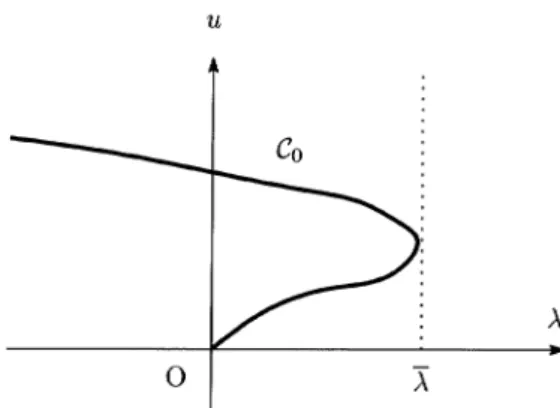
(20) 87. (3). The set. of (Q_{ $\lambda,\ \epsilon$}) around ( $\lambda$, u)=(0,0) consists of a curve ( $\lambda$, u)=( $\lambda$(s), s(1+w(s))) parametrized by s\in(0, $\delta$_{0}) for some $\delta$_{0}>0 In addition, solutions. of positive. ,. $\lambda$. [0, $\delta$_{0})\rightar ow \mathbb{R}. :. and. :. w. .. [0, $\delta$_{0} ) \displaystyle \rightar ow Z=\{u\in C^{2+ $\alpha$}(\overline{ $\Omega$}) : \int_{ $\Omega$}u=0\}. are. continuous. satisfy $\lambda$(0)=0, $\lambda$(s)>0 for s>0 and w(0)=0 Thus bifurcation of positive solutions of (Q_{ $\lambda,\ \epsilon$}) at (0,0) to the region $\lambda$>0 does occur. and. (4) (Q_{ $\lambda,\ \epsilon$}). (5). The. .. ,. has. no. curve. positive solutions for $\lambda$=0 within. unbounded in. further results with. given. ,. on. neighborhood of u=0. ( $\lambda$(s), s(1+w(s))) s\in[0, $\delta$_{0} ), can be of (Q_{ $\lambda,\ \epsilon$}) denoted by C_{ $\epsilon$} so that it is. subcontinuum. Remarks. a. ,. ,. (Q_{ $\lambda,\ \epsilon$}). for $\epsilon$\geq 0. are. extended. as. as. a. in. C(\overline{ $\Omega$}). .. positive solution. (-\infty, $\Lambda$_{ $\epsilon$})\times C(\overline{ $\Omega$}). .. follows.. Remark 5.2.. (1). Assume that. an. a. priori. upper bound for. positive solutions for (Q_{ $\lambda,\ \epsilon$}) exists for C_{ $\epsilon$}>0 such that for any. for any $\mu$>0 there exists a constant positive solution u of (Q_{ $\lambda,\ \epsilon$}) with | $\lambda$|\leq $\mu$ we have every $\epsilon$>0 , i.e.. \Vert u\Vert_{C(\overline{ $\Omega$})}\leq C_{ $\epsilon$)} Then assertions. C_{ $\epsilon$}\}=(-\infty, \overline{ $\lambda$}_{ $\epsilon$}]. We refer to. (2). Assertions. [10]. (1), (2) for. (4). of. Proposition 5.1 ensure that \{ $\lambda$\in \mathbb{R} : ( $\lambda$, u)\in \overline{ $\lambda$}_{ $\epsilon$}\in(0, $\Lambda$_{ $\epsilon$} ]. The inequality (5.2) is still an open question. priori upper bounds for positive solutions of (1.4).. some. for. (1), (2). and. (5.2). a. and. (4). Proposition 5.1 are valid for (P_{ $\lambda$}) Assume that (5.2) C_{ $\epsilon$} is provided uniformly for $\epsilon$\geq O. Then, by the topological analysis proposed by Whyburn [22, Theorem 9.1], we can deduce from Proposition 5.1 that (P_{ $\lambda$}) has a unbounded subcontinuum C_{0} of positive solutions, bifurcating to the region $\lambda$>0 at (0,0) and satisfying \{ $\lambda$\in \mathbb{R} : ( $\lambda$, u)\in C_{0}\}= (-\infty, \overline{ $\lambda$}] as described in Figure 5. This is achieved by considering the limiting behavior of C_{ $\epsilon$} as $\epsilon$\rightarrow 0^{+}. in. .. holds for $\epsilon$=0 , and moreover,. u. FIGURE 5. A unbounded subcontinuum of. the uniform. The. proofs. a. priori. upper bound. (5.2). positive solutions of (P_{ $\lambda$}) when. with respect to $\epsilon$\geq 0 is assumed.. for the results mentioned in this section. are. to appear somewhere else..
(21) 88. REFERENCES. [1]. Fixed point equations and nonlinear eigenvalue problems in ordered Banach spaces, SIAM 18, (1976), 620‐709. A. Ambrosetti, H. Brezis, and G. Cerami, Combined effects of concave and convex nonlinearities in some elliptic problems, J. Funct. Anal. 122, (1994), 519 543. C. Bandle, A.M. Pozio, A. Tesei, Existence and uniqueness of solutions of nonlinear Neumann prob‐ lems, Math. Z. 199, (1988), 257278. K. J. Brown, The Nehari manifold for a semilinear elliptic equation involving a sublinear term, Calc. Var. Partial Differential Equations 22, (2005), 483‐494. K. J. Brown and T.‐F. Wu, A fibering map approach to a semilinear elliptic boundary value problem, Electron. J. Differential Equations 2007, No. 69, (2007), 9\mathrm{p}\mathrm{p}. K. J. Brown and Y. Zhang, The Nehari manifold for a semilinear elliptic equation wit.h a sign‐changing weight function, J. Differential Equations 193, (2003), 481‐499. M. G. Crandall and P. H. Rabinowitz, Bifurcation, perturbation of simple eigenvalues and linearized stability, Arch. Rational Mech. Anal. 52, (1973), 161‐180. D. G. de Figueiredo, Lectures on the Ekeland Variational Principle with Applications and Detours. Tata Inst. Fund. Res. Lectures Math. Phys. 81, Springer (1989) D. G. de Figueiredo, J.‐P. Gossez, P. Ubilla, Multiplicity results for a family of semilinear elliptic problems under local superlinearity and sublinearity, J. Eur. Math. Soc. (JEMS) 8, (2006), 269‐286. J. Garcia‐Azorero, I. Peral, and J. D. Rossi, A convex‐concave problem with a nonlinear boundary condition, J. Differential Equations 198, (2004), 91‐128. J. García‐Melián, J. D. Rossi, and J. C. Sabina de Lis, Limit cases in an elliptic problem with a parameter‐dependent boundary condition, Asympt. Anal. 73, (2011), 147‐168. D. Gilbarg and N. S. Trudinger, Elliptic partial differential equations of second order, Second edition, Springer‐Verlag, Berlin, 1983. C. Morales‐Rodrigo and A. Suárez, Uniqueness of solution for elliptic problems with non‐linear bound‐ ary conditions, Comm. Appl. Nonlinear Anal. 13, (2006), 69‐78. M. H. Protter and H. F. Weinberger, Maximum principles in differential equations, Springer‐Verlag, New York, 1984. H. Ramos Quoirin and K. Umezu, The effects of indefinite nonlinear boundary conditions on the structure of the positive solutions set of a logistic equation, J. Differential Equations 257, (2014), H.. Amann,. Rev.. [2] [3] [4]. [5] [6] [7] [8] [9]. [10]. [11]. [12] [13]. [14] [15]. 3935‐3977.. [16]. Quoirin and K. Umezu, Positive steady states of an indefinite equation with a nonlinear existence, multiplicity and asymptotic profiles, preprint. H. Ramos Quoirin and K. Umezu, Bifurcation for a logistic elliptic equation with nonlinear boundary conditions: A limiting case, J. Math. Anal. Appl. 428, (2015), 1265‐1285. H. Ramos Quoirin and K. Umezu, On a concave‐convex elliptic problem with a nonlinear boundary condition, Ann. Mat. Pura Appl. (4), (2015), online published. H. Ramos Quoirin and K. Umezu, An indefinite concave‐convex equation under a Neumann boundary condition I, preprint. J. D. Rossi, Elliptic problems with nonlinear boundary conditions and the Sobolev trace theorem, Sta‐ tionary partial differential equations, Vol.II, 311‐406, Handb. Differ. Equ., Elsevier/North Holland, Amsterdam, 2005. N. Tarfulea, Existence of positive solutions of some nonlinear Neumann problems, An. Univ. Craiova Ser. Mat. Inform. 23, (1998), 9‐18. G. T. Whyburn, Topological analysis, Second, revised edition, Princeton Mathematical Series, No. 23, Princeton University Press, Princeton, N.J., 1964. T.‐F. Wu, A semilinear elliptic problem involving nonlinear boundary condition and sign‐changing potential, Electron. J. Differential Equations 2006, No. 131, (2006), 15 pp. H. Ramos. boundary. [17] [18] [19] [20]. [21] [22] [23]. condition:. H. RAMOS. UNIVERSIDAD. DE. QUOIRIN. SANTIAGO. DE. CHILE, CASILLA 307, CORREO 2, SANTIAGO, CHILE. E‐mazl address: humberto. [email protected] K. UMEZU DEPARTMENT. OF. MATHEMATICS, FACULTY. E‐mail address:. OF. EDUCATION, IBARAKI UNIVERSITY, MITO 310‐8512, JAPAN. [email protected].
(22)
図
関連したドキュメント
This article studies the existence, stability, self-similarity and sym- metries of solutions for a superdiffusive heat equation with superlinear and gradient nonlinear terms
We shall consider the Cauchy problem for the equation (2.1) in the spe- cial case in which A is a model of an elliptic boundary value problem (cf...
We study the existence of positive solutions for a fourth order semilinear elliptic equation under Navier boundary conditions with positive, increasing and convex source term..
In order to get a family of n-dimensional invariant tori by an infinitely dimensional version of KAM theorem developed by Kuksin [4] and Pöschel [9], it is necessary to assume that
Lagnese, Decay of Solution of Wave Equations in a Bounded Region with Boundary Dissipation, Journal of Differential Equation 50, (1983), 163-182..
Ntouyas; Existence results for a coupled system of Caputo type sequen- tial fractional differential equations with nonlocal integral boundary conditions, Appl.. Alsaedi; On a
F igueiredo , Positive solution for a class of p&q-singular elliptic equation, Nonlinear Anal.. Real
Y ang , The existence of a nontrivial solution to a nonlinear elliptic boundary value problem of p-Laplacian type without the Ambrosetti–Rabinowitz condition, Non- linear Anal.
