Difference Approximation to Aubry-Mather Sets (Dynamical Systems : with Hyperbolicity and with Large Freedom)

Difference

_{Approximation to Aubry-Mather Sets}

Kohei Soga

Waseda University

([email protected])

1

_{PDE Approach to the Aubry-Mather}

_Theory

This paper presents a rough description of the PDE approach to the Aubry-Mather

theory and the results of the preprint [9] by Takaaki Nishida and the author on difference

approximation to Aubry-Mather sets.

We consider the following

non-autonomous

Hamiltonian systems with

one

degree of

freedom

generated by $C^{2}$

-functions

_$H$:

(1.1) $x’(s)=H_{u}(x(s), s, u(s))$_, $u’(s)=-H_{x}(x(s), s, u(s))$_,

$H(x, s, u):\mathbb{T}\cross \mathbb{T}\cross \mathbb{R}arrow \mathbb{R},$ $\mathbb{T}:=\mathbb{R}/\mathbb{Z}$

.

A physical example of (1.1) is

a

forced pendulum with

a

time-periodic force. Under

several conditions,

_{autonomous Hamiltonian}

systems with two degrees of freedom

can

be

deduced

to (1.1)

on

each energy level set.

Since $H(x, s, u)$ is periodic with respect to $s$ with the period 1, the dynamics of (1.1)

can

be studied by the iteration of its time-l map

$\mu=\phi_{H}^{0,1}$ : _{$\mathbb{T}\cross \mathbb{R}\ni(x(O), u(O))\mapsto(x(1), u(1))\in \mathbb{T}\cross \mathbb{R}$},

where $\phi_{H}^{0,s}$ is the flow of

(1.1).

Figure 1 shows

a

numerical example of the trajectories $(x^{k}, u^{k})=\mu^{k}(x^{0}, u^{0}),$ $k\in \mathbb{N}$

.

X

In Figure 1

we

observe the several smooth

curves

diffeomorphic to $\mathbb{T}$ which trap the

trajectories. Such

curves are

called $\mu$-invariant tori. We also observe the region where

only

one

trajectory

seems

to

move

around densely. Such a region is sometimes called

a

chaotic region.

We focusour attention

on

the searchfor $\mu$-invarianttori or,

more

generally, $\mu$-invariant

sets, where $\mathcal{I}\subset \mathbb{T}\cross \mathbb{R}$ is said to be

$\mu$-invariant, if $\mu(\mathcal{I})\subset \mathcal{I}$. This is

one

of the

central issues in the theory of Hamiltonian dynamics and has been studied theoretically

and numerically for

a

long time. The celebrated results

on

the issue

are

the KAM

(Kolmogorove-Arnold-Moser) theory and Aubry-Mather theory for

area

preserving twist

maps

on an

annulus. Although these theories

cover

also the flow cases,

we

will not refer

to this here.

The KAM theory applies in particular to slightly perturbed integrable twist maps.

Suppose that $\mu$ is smooth as needed and is of the form $\mu(x, u)=\mu_{0}(x, u)+\mu_{1}(x, u)$

with $\mu_{0}(x, u)=(x+\rho(u), u),$ $\rho’(u)\neq 0$ and $|\mu_{1}(x, u)|\ll 1$

on

$\mathbb{T}\cross[u_{1}, u_{2}]$. Then the

KAM

theory provides

a

family

of

$\mu$

-invariant

tori

called KAM

tori

which

occupies

a

large

part of $\mathbb{T}\cross[u_{1}, u_{2}]$

.

Each KAM torus carries quasi-periodic trajectories with

a

common

asymptotic slope $\alpha=\lim_{|k|arrow\infty}\frac{\tilde{x}^{k}}{k}$ ($\tilde{x}^{k}\in \mathbb{R}$ is the lift of$x^{k}\in \mathbb{T}$) called

a

rotation number,

which is

a

Diophantine number. The KAM theory is

a

kind of perturbation theory

and requires

a severe

smallness condition for the perturbation and

a

number theoretical

condition. Numerical studies show that KAM tori disappear and chaotic regions spread

as

the magnitude of perturbation gets larger, in general. It is

an

interesting problem to

make this process clear.

The Aubry-Mather theory is not based on

a

perturbation theory but

on

calculus of

variation and does not require the smallness condition

nor

the number theoretical

con-dition. Suppose that $\mu$ satisfies the twist condition, namely, $\mu(x, u)=(f(x, u), g(x, u))$

with $f_{u}(x, u)\neq 0$

.

Then the Aubry-Mather theory provides

a

family of $\mu$-invariant sets

calledAubry-Mather sets. EachAubry-Mather set is either

a

smooth

curve

diffeomorphic

to $\mathbb{T}$

or

a subset of a Lipschitz curve homeomorphic to $\mathbb{T}$ and carries conditionally

peri-odic trajectories with

a

common

rotation number $\alpha$, namely, if$\alpha$ is rational (irrational),

the trajectories

are

periodic (quasi-periodic). The remarkable fact is that not only for

Diophantine numbers but also for any number $\alpha$ there exists the Aubry-Mather set with

the rotation number $\alpha$. We refer to [7] for

an

interesting review of the Aubry-Mahter

theory.

J. Moser pointed out that each

area

preservingtwist map on

an

annulus is represented

as

thetime-l mapof

a

certain Hamiltonian system ofthe form (1.1) with $H(x, s, u)$ which

is strictly

convex

in $u[7]$ (see also its reference [28]). Let

us

remark that the

converse

is

not true.

A

new

approach to the Aubry-Mather theory is pioneered independently by A. Fathi

[5] and W. $E[4]$

.in

combination with the analysis of Hamilton-Jacobi equations. Let

us

call the new approach the “PDE approach”. Fathi deals with autonomous Hamiltonian

systems with general degrees offreedom; His setting is different from

ours.

We focus

our

attention to the results of $E$, which deal with (1.1) for $H(x, s, u)$ which is strictly

convex

in $u$. $E$ shows that for each number $\alpha$ there exists a $\mu$-invariant set with the rotation

number $\alpha$ which is

a

subset of the graph of

a

solution to

a

nonlinear PDE and has

a

structure quite similar to that of Aubry-Mather sets. This result is independent of the

The PDE approach

can

be

seen as a

generalization of

a

consequence ofthe “method of

characteristics”

for

first

order nonlinear PDEs. Let

us

consider the initial value problem

to the hyperbolic conservation law with $C^{1}$-initial data

(1.2) $\{\begin{array}{l}u_{t}(x, t)+H(x, t, u(x, t))_{x}=0 in \mathbb{R}^{2},u(x, 0)=u_{0}(x) on \mathbb{R}.\end{array}$

Let $(\tilde{x}(s;y), u(s;y))$ : $\mathbb{R}arrow \mathbb{R}^{2}$ be the solution of

$\tilde{x}’(s)=H_{u}(\tilde{x}(s), s, u(s)),$ $u’(s)=-H_{x}(\tilde{x}(s), s, u(s))$, $\tilde{x}(0)=y,$ $u(O)=u_{0}(y)$.

The

curve

$c(s;y)$ $:=(\tilde{x}(s;y), s, u(s;y))$ is called

a

characteristic curve of (1.2). The idea

of the method of characteristics is the following: If for each $x,$$t$ there exists the unique

value

$y=y(x, t)$

_{for which}

$\tilde{x}(t;y)=x$

and the

family

of characteristic

curves

$\{c(s;y)\}_{y\in \mathbb{R}}$

forms a

$C^{1}$-surface

of

the _{$(x, t, u)$}-space represented

as

$u=u(x, t)$ $:=u(t;y(x, t))$, then

$u(x, t)$ is the$C^{1}$-solution of(1.2). Conversely, ifthereexists

a

$C^{1}$-solution $u(x, t)$ of(1.2),

then the surface defined

as

the graph of $u(x, t)$ consists of the family of characteristic

curves.

As

a

consequence,

we

have the following statement:

Proposition 1.1 Suppose that there exists

a

$\mathbb{Z}^{2}$

-periodic $C^{1}$-solution _{$\overline{u}(x, t)$}

of

(13) $u_{t}(x, t)+H(x, t, u(x, t))_{x}=0$.

Then $\mathcal{I}(\overline{u});=\{(x,\overline{u}(x, 0))|x\in \mathbb{T}\}$ is a $\mu$-invariant torus which carries trajectories with

a common

rotation number.

The proof is simple. Let $(x^{0}, u^{0})$ be any point of$\mathcal{I}(\overline{u})$ and $\tilde{x}(s)$ be the solution of

$\tilde{x}’(s)=H_{u}(\tilde{x}(s), s,\overline{u}(\tilde{x}(s), s)),\tilde{x}(0)=x^{0}$.

Note that $u^{0}=\overline{u}(x^{0},0)$ and $\tilde{x}(s)$

can

be defined globally

on

$\mathbb{R}$

.

Then using (1.3)

we

have

$\frac{d}{ds}\overline{u}(\tilde{x}(s), s)$ _$=$ $\overline{u}_{t}(\tilde{x}(s), s)+\overline{u}_{x}(\tilde{x}(s), s)\tilde{x}’(s)$

$=$ $\overline{u}_{t}(\tilde{x}(s), s)+H_{u}(\tilde{x}(s), s,\overline{u}(\tilde{x}(s), s))\overline{u}_{x}(\tilde{x}(s), s)$

$=$ $-H_{x}(\tilde{x}(s), s,\overline{u}(\tilde{x}(s), s))$.

Therefore $(x(s), u(s))$ $:=(\tilde{x}(s)mod 1,\overline{u}(\tilde{x}(s), s))$ is

a

solution of (1.1). By the $\mathbb{Z}^{2}-$

periodicity of $\overline{u}$

we

have $\mu^{k}(x^{0}, u^{0})=(x(k), u(k))=(x(k),\overline{u}(x(k), 0))\in \mathcal{I}(\overline{u})$ for any

$k\in \mathbb{Z}$

.

We

see

also that $X(s)$ $:=(x(s), smod 1)$ : $\mathbb{R}arrow \mathbb{T}^{2}$ is either periodic

or

one-to-one. Thus

we

conclude that there exists $\lim_{|s|arrow\infty}\frac{\overline{x}(s)}{s}$ which is independent of

the point $(x^{0}, u^{0})\in \mathcal{I}$, due to the classical result of Poincar\’e: Let $y(s)$ : $\mathbb{R}arrow \mathbb{R}$ be

continuous such that $Y(s)$

$:=(y(s)mod 1, smod 1)$

: $\mathbb{R}arrow \mathbb{T}^{2}$ is either periodic

or

one-to-one. Then there exists the asymptotic slope $\lim_{|s|arrow\infty}\frac{y(s)}{s}$ which is

finite.

If,

for

another$\tilde{y}(s)$ : $\mathbb{R}arrow \mathbb{R}$ satisfying the above condition, $\tilde{Y}(s)$ and$Y(s)$

never

intersect, then

their asymptotic slopes

are

the

same.

Wecannot always expect theexistence of$\mathbb{Z}^{2}$

-periodic$C^{1}$-solutions$\overline{u}(x, t)$. The method

of characteristics is technically limited to construction

of

local in time $C^{1}$-solutions. It

case

where characteristic

curves

are

always defined globally, because the surface

formed

by the characteristic

curves

may be eventually folded and it cannot be represented

as

the

graph

of a

single

valued function.

In other words, the

curves

$(\tilde{x}(s;y), s)$ : $\mathbb{R}arrow \mathbb{R}^{2}$,

which

are

called the projected characteristic curves, may eventually have intersections

with others in finite time. That is why the class of entropy solutions is introduced.

Entropy solutions

are

special weak solutions of (1.3) with

an

additional condition called

the entropy condition.

Now

we

consider $\mathbb{Z}^{2}$-periodic

solutions of (1.3) in the class of entropy solutions. A

function $\overline{u}(x, t)$ is

a

$\mathbb{Z}^{2}$

-periodic entropy solution of (1.3) with $H(x, s, u)$ which _is

convex

in $u$, if$\overline{u}$ belongs to $L_{loc}^{1}(\mathbb{R}^{2})$ and satisfies the following:

.

$\overline{u}(x+k, t+l)=\overline{u}(x, t)$ for any _$x,$$t\in \mathbb{R}$ and $k,$ $l\in \mathbb{Z}$,

.

$\iint_{\mathbb{R}^{2}}\overline{u}(x, t)\varphi_{t}(x, t)+H(x, t,\overline{u}(x, t))\varphi_{x}(x, t)dxdt=0$

for any

$\varphi\in C_{0}^{\infty}(\mathbb{R}^{2})$,

.

$\overline{u}(x+h, t)-\overline{u}(x, t)\leq e(t)h$

for any

$h>0$ and _$x,$ $t\in \mathbb{R}$,

where $C_{0}^{\infty}(\mathbb{R}^{2})$ denotes the setof$C^{\infty}$-functions defined

on

$\mathbb{R}^{2}$ with

compact supports and

$e(t)$ is

a

positive valued function. The last condition is the so-called _{entropy condition}

for the

convex

case.

Countably many discontinuities

are

allowed for $\overline{u}(\cdot, t)|_{x\in T}$ for each

fixed

$t$, but they must jump down! A set of points _{$x_{0}=x_{0}(t)$} of discontinuity of

$\overline{u}(\cdot, t)$

form

a

continuous

curve for

$t\in(t_{0}, \infty)$, which is called

a

shock.

The problems here

are

the following: How to find $\mathbb{Z}^{2}$

-periodic entropy solutions of

(1.3)? Is there any result similar to Proposition 1.1 in the class of entropy solutions?

For simplicity

we

consider these problems taking

a

simple example of

$H(x, s, u)= \frac{1}{2}u^{2}-F(x, s)$

.

In this

case

(1.1) is of the form

(1..4) $x’(s)=u(s)$, $u’(s)=F_{x}(x(s), s)$

and (1.3) is the

forced

Burgers equation with the $\mathbb{Z}^{2}$

-periodic forcing term $F_{x}(x, t)$

(15) $u_{t}(x, t)+u(x, t)u_{x}(x, t)=F_{x}(x, t)$

.

The arguments below hold for general functions $H(x, s, u)$ _{which is strictly}

_convex

_and

superlinear with respect to $u$ (see e.g. [2], [1]).

H. R. Jauslin, H. O. Kreiss and J. Moser [6] prove that there exist $\mathbb{Z}^{2}$-periodic entropy

solutions of (1.5) throughthe vanishing viscositymethod and conjecture that $\mathcal{I}(\overline{u})$ would

contain

a

$\mu$-invariant set $\mathcal{M}(\overline{u})$

for

each $\mathbb{Z}^{2}$-periodic entropy solution

$\overline{u}$

of

(1.5).

Jauslin-Kreiss-Moser

take the following steps to obtain $\mathbb{Z}^{2}$

-periodic entropy

solutions: First

they

find

$\mathbb{Z}$-periodic in $t$ solutions $\overline{u}^{\nu}$ of the parabolic equation with the periodic

boundary condition

(16) $u_{t}^{\nu}(x, t)+u^{\nu}(x, t)u_{x}^{\nu}(x, t)=F_{x}(x, t)+\nu u_{xx}^{\nu}(x, t)$ in $\mathbb{T}\cross \mathbb{R}_{+}$,

where the term $\nu u_{xx}^{\nu},$ $\nu>0$is called

an

artificialviscosity, whichyieldsclassical solutions

to (1.6). And then theyfind

a

sequence $\nu_{j}arrow 0+$ for which$\overline{u}^{\nu_{j}}$ convergesto

a

$\mathbb{Z}^{2}$-periodic

entropy solution $\overline{u}$ of (1.5). Note that each classical solution of(1.6)

conserves

its

average

on

$\mathbb{T}:\int_{0}^{1}u^{\nu}(x, t)dx\equiv C$for $t>0$, and

so

does each entropy solution of (1.5) in

$\mathbb{T}\cross \mathbb{R}_{+}$

.

Theorem 1.2 ([6]) 1. Fix $\nu>0$ arbitmrily. Then

for

_each $C\in \mathbb{R}_{f}$ there exists the

$u\dot{n}ique$ time-periodic $C^{2}$-solution $\overline{u}^{\nu}$

of

(1.6) with the momentum

C.

Any other solutions

$u^{\nu}$

of

(1.6) with the

same

momentum _$C$

satisfy

1

$u^{\nu}(\cdot, t)-\overline{u}^{\nu}(\cdot, t)\Vert_{L^{1}(T)}arrow 0$

as

$tarrow\infty$.

2. For each $C\in \mathbb{R}$ there exists a sequence _{$\nu_{j}arrow 0+such$} that the sequence $\overline{u}^{\nu_{j}}$ with

the momentum $C$ converges to a $\mathbb{Z}^{2}$

-periodic entropy solution $\overline{u}$

of

(1.5) in the topology

of

$C^{0}(\mathbb{T};L^{1}(\mathbb{T}))$, which belongs to Lip$(\mathbb{T};L^{1}(\mathbb{T}))$ and has the momentum C. Furthermore

$\overline{u}$ is uniformly bounded

and $\overline{u}(\cdot, t)|_{x\in T}$ is a

function of

bounded variation

for

each $t$.

The conjecture ofJauslin-Kreiss-Moser above is proved to hold by $E[4]$: There exists a

$\mu$-invariant closed subset $\mathcal{M}(\overline{u})$

of

$\mathcal{I}(\overline{u})$ carwing the conditionally periodic trajectories

with a

common

rotation number. $\mathcal{I}(\overline{u})$ is backward

$\mu$-invariant. The remaining part

$\mathcal{I}(\overline{u})\backslash \mathcal{M}(\overline{u})$ is the unstable set

of

$\mathcal{M}(\overline{u})$, namely,

any

backward trajectories

of

$\mu$

on

the graph fall into $\mathcal{M}(\overline{u})$.

As

is

discussed

below, the last

fact

is important also for the

computation of $\mathcal{M}(\overline{u})$.

Before stating

more

details

we

see

that the results are natural consequences of

prop-erties of entropy solutions. Let

us

consider the situation where $\overline{u}$ is piecewise $C^{1}$ and

$\overline{u}(\cdot, t)|_{x\in T}$ has

a

certain finite number of points of discontinuity for each $t$. The smooth

part of graph$(\overline{u})$ _{$:=\{(x, t,\overline{u}(x, t))|x, t\in \mathbb{T},\overline{u}(x-0, t)=\overline{u}(x+0, t)\}$} consists of the

characteristic

curves.

The projected characteristic

curves

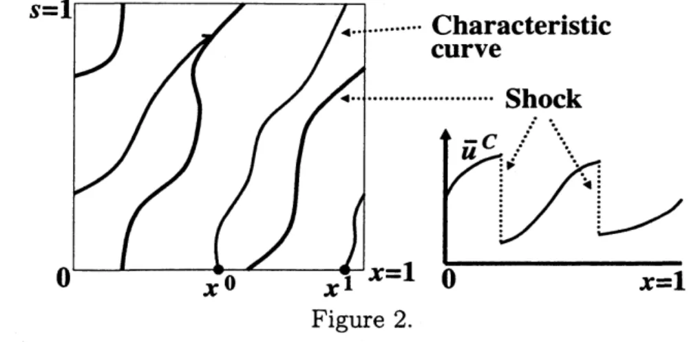
have the velocity $(\overline{u}(x(t), t), 1)$.

For a point $x_{0}$ ofdiscontinuity of $\overline{u}(\cdot, t_{0})$, we have a positive number $d>0$ such that

$\overline{u}(x_{0}-h, t_{0})>\overline{u}(x_{0}+h, t_{0})+d$ for any small $h\geq 0$. Hence the twoprojected characteristic

curves

through $(x_{0}-h, t_{0})$ and $(x_{0}+h, t_{0})$ necessarily intersect at $s>t_{0}$

on

a

shock and

these

characteristic

curves

go

away from graph$(\overline{u})$

.

The situation is illustrated

on

$\mathbb{T}^{2}$

in

Figure 2.

For $s<t_{0}$, on the other hand, each characteristic

curve never

runs into any shocks.

In other words, two projected characteristic curves never intersect for $s<t_{0}$, because

otherwise the entropy condition is violated at the intersection. Therefore any

character-istic

curve

$c(s)=(\tilde{x}(s), s, u(s))$ through a point of the smooth part of graph$(\overline{u})$ at $s=t_{0}$

stay

on

the smooth part for $s<t_{0}$, namely, $u(s)=\overline{u}(\tilde{x}(s), s)$ for $s<t_{0}$.

That is why $\mathcal{I}(\overline{u})$ is only backward

$\mu$-invariant in general. For each characteristic

curve

there exist accumulating points $x^{*}$ of _{$\{\tilde{x}(-k)mod 1\}_{k\in \mathbb{N}}$}, which

are

the points

of continuity of $\overline{u}(\cdot, 0)$

.

Therefore we conclude that the characteristic

curves

through

$(x^{*}, 0,\overline{u}(x^{*}, 0))$

never

run

into any shocks in both directions. These special points

$(x^{*}, 0,\overline{u}(x^{*}, 0))$ yield

a

$\mu$-invariant set $\mathcal{M}(\overline{u})$.

The above speculation

can

be justified through the theory of viscosity solutions of the

Hamilton-Jacobi

equations of the form

(1.7) $v_{t}(x, t)+H(x, t, v_{x}(x, t))=$ const.

We briefly refer to the notion of viscosity solutions. If

we

have

a

$C^{1}$-solution $v(x, t)$

of (1.7) defined

on

$\mathbb{R}\cross \mathbb{R}_{+}$, then multiplying the derivative $\varphi_{x}$ of

any

test function

$\varphi\in C_{0}^{\infty}(\mathbb{R}\cross \mathbb{R}_{+})$ and integrating by parts

over

$\mathbb{R}\cross \mathbb{R}_{+}$

we

have

a

continuous weak

solution $u=v_{x}$ of (1.3). The regularity ofentropy solutions

on

$\mathbb{R}\cross \mathbb{R}_{+}$ is

worse

than $C^{0}$

in general. Therefore we cannot always expect such a solution of (1.7). Note that the

method ofcharacteristics also works for the construction of local in time $C^{2}$-solutions of

(1.7) with $C^{2}$-initial data.

Let

$u(x, t)\in L^{\infty}(\mathbb{R}\cross \mathbb{R}_{+};\mathbb{R})$ be

a

weak solution

of

(1.3) which belongs also to

$Lip_{loc}(\mathbb{R}_{+};L^{1}(K;\mathbb{R}))$ for each compact set $K\subset \mathbb{R}$

.

Then

we

have

a

locally Lipschitz

function $v$ of the form $v(x, t)= \int_{0}^{x}u(y, t)dy+\int_{0}^{t}P(s)ds$ with

some

function $P(s)$ which

is defined

on

$\mathbb{R}\cross \mathbb{R}_{+}$ and satisfies (1.7) almost everywhere. Note that

a

locally Lipschitz

function is differentiable almost everywhere. If $u$ satisfies the entropy condition, then

$v(\cdot, t)$ for each fixed $t$ has

a

special property in its nondifferentiable part which is called

semiconcavity. Satisfaction ofthe equation almost everywhere and semiconcavity

are

the

characterizations of viscosity solution of (1.7), which

are

also realized by the vanishing

viscosity method with the artificial viscosity $\nu v_{xx}$. We point out [3], [1] for

more

details.

Now we see

some

details of the results by E. Let $\overline{u}(x, t)$ be a $\mathbb{Z}^{2}$

-periodic entropy

solution of (1.5) with the momentum $C$. It follows from the above argument that there

exists

a

$\mathbb{Z}^{2}$-periodic Lipschitz function

$\overline{v}(x, t)$ satisfying $C+\overline{v}_{x}=\overline{u}$

a.e.

such that

$\overline{v}_{t}(x, t)+H(x, t, C+\overline{v}_{x}(x, t))=\overline{H}(C)$ in $\mathbb{R}^{2}$ (in the

sense

of viscosity solution),

$\overline{H}(C)=\int\int_{T^{2}}H(x, t,\overline{u}(x, t))dxdt$

.

Let $L^{C}(x, t, \xi)$ be the Legendre transform of $H(x, t, C+p)$ with respect to _$p$

.

The

well-known representation formula for viscosity solutions yields

(1.8) $\overline{v}(x, t)=\inf_{\eta\in AC,\eta(t)=x}\{l^{t}L^{C}(\eta(s), s, \eta’(s))ds+\overline{v}(\eta(\tau), \tau)\}+\overline{H}(C)(t-\tau)$,

where $AC$ is the class of absolutely continuous

curves

$\eta$ :

$\mathbb{R}arrow \mathbb{R}$ and $\tau$ is

an

arbitrary

number less than $t$. This is

a

direct generalization of the representation

formula

for

local in time $C^{2}$-solutions via the method of characteristics. The variational problem

in (1.8) is denoted by $($CV$)_{\tau}^{x,t}$. There exists

a

$C^{2}$-minimizer

$\gamma$ : $[\tau, t]arrow \mathbb{R}$ of $($CV$)_{\tau}^{x,t}$

satisfying the Euler-Lagrange equation with respect to $L^{C}$. Therefore $(x(s), u(s))$

$:=$ $(\gamma(s)mod 1, C+L_{\xi}^{c}(\gamma(s), s, \gamma’(s))):[\tau, t]arrow \mathbb{T}\cross \mathbb{R}$ satisfies (1.4).

Theorem 1.3 $([$4$])$ 1. Existence

of

“one-sided minimizers”: For each $(x,$ $t)\in \mathbb{R}^{2}$ there

exists

a

curve

$\gamma(s)$ : $(-\infty, t]arrow \mathbb{R}$ with $\gamma(t)=x$ such that

for

any interval $[t_{1}, t_{0}]\subset$

$(-\infty, t]$ the restnction $\gamma|_{[t_{1},t_{0}]}$ is

a

minimizer

of

$(CV)_{t_{1}}^{\gamma(t_{0}),t_{0}}$ and $\overline{v}$ is

differentiable

with

respect to $x$ at each point $(\gamma(s), s)$ with $s<t$ satisfying

If

there exists $v.(x, t)$_{, then (1.9) holds}

for

$s=t$ and such $\gamma$ is unique.

2. Existence

_of

$l$

‘two-sided minimizers”: There exist

curves

$\gamma^{*}(s)$ : $\mathbb{R}arrow \mathbb{R}$ such that

for

any interval $[t_{1}, t_{0}]\subset \mathbb{R}$ the restriction $\gamma^{*}|_{[t_{1},t_{0}]}$ is a minimizer

of

$(CV)_{t_{1}}^{\gamma^{*}(t_{0}),t_{0}}$ and

$\overline{v}$

is

_{differentiable}

with respect to $x$ at each point $(\gamma^{*}(s), s)$ with $s\in \mathbb{R}$ satisfying

$\overline{v}_{x}(\gamma^{*}(s), s)=L_{\xi}^{C}(\gamma^{*}(s), s, \gamma^{*}’(s))$.

3. $\overline{H}(C)$ depends only on $C$ and belongs to $C^{1}(\mathbb{R}).\overline{H}’(C)$ is monotone increasing.

Each

one

and two-sided minimizer$\gamma,$$\gamma^{*}$

satisfies

$\lim_{sarrow-\infty}\frac{\gamma(s)}{s}=\overline{H}’(C)$, $\lim_{|s|arrow\infty}\frac{\gamma^{*}(s)}{s}=\overline{H}’(C)$ .

The following

are

characteristic

curves

of (1.5) in $\mathbb{T}^{2}$:

$c(s)=(\gamma(s)mod 1, smod 1, C+\overline{v}_{x}(\gamma(s), s))$ : $(-\infty, t]\cdotarrow \mathbb{T}^{2}\cross \mathbb{R}$, $c^{*}(s)=(\gamma^{*}(s)mod 1, smod 1, C+\overline{v}_{x}(\gamma^{*}(s), s))$ : $\mathbb{R}arrow \mathbb{T}^{2}\cross \mathbb{R}$

.

They

are

trapped

on

graph$(\overline{u})=$

{

$(x,$$t,$ $C+\overline{v}_{x}(x,$ $t))|x,$$t\in \mathbb{T}$, there exists $\overline{v}_{x}(x,$ $t)$

}.

In

other words, if

a

characteristic

curve

$c(s)$ of (1.5) in $\mathbb{T}^{2}$ satisfies _{$c(t_{0})\in$} graph$(\overline{u})$ for

some

$t_{0}\in \mathbb{R}$, then $c(s)$ is trapped

on

graph$(\overline{u})$ for $s\leq t_{0}$

.

Let $\Omega(\gamma)$ be the set of all

the $\omega$-limit points of $\{\gamma(-k)mod 1|k\in \mathbb{N}, -k\leq t_{0}\}$, where $\gamma$ : $(-\infty, t_{0}]arrow \mathbb{R}$ is

a

one-sided minimizer of (1.8). Each one-sided minimizer through

a

point of $\Omega(\gamma)$

can

be

extended to a two-sided minimizer. We define

$\Gamma(\overline{u})$ $:=\{(\gamma^{*}(s)mod 1,$ $smod 1,$

$C+ \overline{v}_{x}(\gamma^{*}(s), s))|\gamma^{*}(0)\in\bigcup_{\gamma}\Omega(\gamma),$ $s\in \mathbb{R}\}$ ,

where $\gamma^{*}$

are

two-sided minimizers. $\Gamma(\overline{u})$ is

a

subset of graph$(\overline{u})$. It is proved in [4] that

for each one-sided minimizer $\gamma$ there exists

a

two-sided minimizer

$\gamma^{*}$ such that

(1.10) $|\gamma(s)-\gamma^{*}(s)|arrow 0$

as

$sarrow-\infty$

and therefore each$c(s)$ trapped

on

graph$(\overline{u})$ for $s\leq t_{0}$ falls into $\Gamma(\overline{u})$

as

$sarrow-\infty$

.

This is

based

on

thesimple factthat, fortwodifferent minimizers $\gamma,\tilde{\gamma}$

associated

with$\overline{u},$ $(\gamma(s), s)$

and $(\tilde{\gamma}(s), s)$

never

intersect. For $sarrow+\infty$, each $c(s)$ through

a

point ofgraph$(\overline{u})\backslash \Gamma(\overline{u})$

runs

into

a

shock and goes away from graph$(\overline{u})$ in general. $\mathcal{M}(\overline{u})$ $:=\Gamma(\overline{u})\cap(\mathbb{T}\cross\{0\}\cross \mathbb{R})$

is a $\mu$-invariant set carrying the trajectories of $\mu$ with the rotation number

$\overline{H}’(C)$. For

any $\alpha\in \mathbb{R}$, there exists $C$ such that $\overline{H}’(C)=\alpha$. As is proved in [4], $\mathcal{M}(\overline{u})$ is

a

closed

subset of

a

Lipschitz

curve.

We call $\mathcal{M}(\overline{u})$ the Aubry-Mather set associated with the

entropy solution $\overline{u}$. From

now

on, the term ”Aubry-Mather set”

means

$\mathcal{M}(\overline{u})$

.

2

Difference Approximation

to

Aubry-Mather

sets

Let

us

consider the computational aspects

of

the issue. The main interest is the

compu-tation of $\mathbb{Z}^{2}$

-periodic entropy

solutions

of (1.5) and Aubry-Mather sets. As

an

effective

approach to entropy solutions,

we

have not only the smooth approximation by the

convenient

also

for

numerical

simulations.

The rigorous treatment

of

the

difference

ap-proximation to entropy solutions is found in lots of works (e.g. [8]). Many of them

are

on

entropy solutions of initial value problems.

Concerning the difference approximation of periodic entropy solutions,

we

find in

[6]

a

difference scheme to (1.6) for numerical tests of Theorem 1.2 (but there is

no

theoretical argument for the scheme). We also point out [10], in which the existence of

$\mathbb{Z}^{2}$

-periodic entropy solutions of (1.5) is proved with the Lax-Friedrichs difference scheme

and Brouwer’s fixed point theorem. The idea is to regard $\mathbb{Z}^{2}$-periodic

difference solutions

as fixed points of the time-l map derived from the semigroup of the difference scheme.

Wepresent two methods which

are more

constructive and easily simulated [9]: The

one

is

based

on

the long time

behavior of

_{difference solutions derived from the Lax-Friedrichs}

difference

scheme. The other is based

on

Newton’s method for the

fixed

points

of

the

time-l map. The

convergence

of these methods

are

established. Our results

can

be

extended to general types of the forced Burgers equation (1.3) with $H(x, s, u)$ _{which is}

strictly

convex

in $u$, assuming additional conditions.

We construct $\mathbb{Z}^{2}$-periodic

entropy solutions of the forced Burgers equation (1.5) with

a

$\mathbb{Z}^{2}$

-periodic $C^{2}$-function _$F$.

Our

basic tool is the two-step

Lax-Riedrichs difference

scheme in $\mathbb{T}\cross \mathbb{R}_{t\geq 0}$. Let $N,$ $K$ be natural numbers. The mesh size is defined

as

$\Delta x:=$

$N^{-1},$ $\triangle t$ $:=K^{-1}$

.

Set $\lambda$ _{$:=\Delta t/\triangle x,$}

$x_{n}$ $:=n\triangle x\in[0,1](n=0,1,2, \cdots, N),$ $t_{k}$ $:=k\Delta t\in$ $[0, +\infty)(k=0,1,2, \cdots)$. The solution _{to the initial value problem}

$\{\begin{array}{l}u_{t}(x, t)+u(x, t)u_{x}(x, t)=F_{x}(x, t) in \mathbb{T}\cross \mathbb{R}_{+},u(x, 0)=g(x) on \mathbb{T}\end{array}$

is replaced with the family of vectors

$u^{k}=(u_{0}^{k}, u_{1}^{k}, \cdots, u_{N-1}^{k})\in \mathbb{R}^{N}(k=0,1,2, \cdots)$,

where $u^{0}=(g(x_{0}), \cdots, g(x_{N-1}))$

.

This is called the

difference

solution with the _initial

value $u^{0}$. Each

difference

solution $u^{k}$ with an initial value $u^{0}\in \mathbb{R}^{N}$ is given in the

following way: Let $\Delta y$ $:= \frac{1}{2}\Delta x,$ $\triangle\tau$ _{$:= \frac{1}{2}\Delta t,$}

$y_{m}$ $:=m\triangle y\in[0,1](m=0,1,2, \cdots, 2N)$,

$\tau_{l}$ $:=l\Delta\tau\in[0, +\infty)(l=0,1,2, \cdots)$;Define

$u_{n}^{k}:=W_{2n}^{2k}.$,

where $W_{m}^{l}$

are

computed for each $l=0,1,2,$ $\cdots$ and each$m\in\{0,1,2, \cdots, 2N\}$ satisfying

$l+m=$

even

through the difference equation with the periodic boundary condition

$\{\begin{array}{l}\frac{W_{m+1}^{l+1}-\frac{(W_{m+2}^{l}+W_{m}^{l})}{\Delta\tau 2}}{}+\frac{1}{2}\frac{(W_{m+2}^{l})^{2}-(W_{m}^{l})^{2}}{2\Delta y}=\frac{F(y_{m+2},\tau_{l})-F(y_{m},\tau_{l})}{2\Delta y},W_{\pi\dot{\iota}\pm 2N}^{l}=W_{m}^{l}, W_{2n}^{0}=u_{n}^{0}.\end{array}$

Set

$u_{n\pm N}^{k}$ $:=u_{n}^{k}$

.

The semigroups $u^{0}\mapsto u^{k},$ $W^{0}\mapsto W^{\iota}$

are

denoted by $\psi^{k}$ : $\mathbb{R}^{N}arrow \mathbb{R}^{N}$,

$\Psi^{l}$

:

$\mathbb{R}^{N}arrow \mathbb{R}^{N}$ respectively. $\psi^{k},$ $\Psi^{l}$

are

$C^{2}$.

Since

_$F$ is $\mathbb{Z}^{2}$

-periodic,

the

time-l

map

is

well-defined.

Note that $\psi^{KT+k}=\psi^{k}$_. $\circ\phi^{T}$ for each $T\in \mathbb{N}$, where $\phi^{T}$ is the T-iteration

of $\phi$. The following

function

is called

an

approximate solution of (1.5) in

$\mathbb{T}\cross \mathbb{R}_{\geq 0}$:

$u_{\triangle}(x, t):= \frac{u_{n+1}^{k}-u_{n}^{k}}{\triangle x}(x-x_{n})+u_{n}^{k}$ for

$x\in[x_{n}, x_{n+1}],$ $t\in[t_{k}, t_{k+1}),$ $\triangle=(\triangle x, \triangle t)$

.

It follows from a simple calculation that the average in $x$ of each difference solution $u^{k}$

at each $k$ and therefore that of the approximatesolution

$u_{\Delta}(x, t)$ is conservative, namely

$C(u^{0}):= \sum_{n=0}^{N-1}u_{n}^{0}\triangle x\equiv\sum_{n=0}^{N-1}u_{n}^{k}\Delta x\equiv\int_{0}^{1}u_{\Delta}(x, t)dx$

.

The value $C=C(u^{0})$ _{is called the momentum of}

_a

_solution. $u^{k}(C),$$u_{\Delta}^{C}(x, t)$ denote

$u^{k},$$u_{\Delta}(x, t)$ with the momentum C. $u^{k}$ is said to be

a

periodic difference solution, if

$u^{k+K}=u^{k}$ _{for all $k=0,1,2,$} $\cdots$

.

This is equivalent to the relation $\phi(u^{0})=u^{0}$

.

For each $v=(v_{0}, \cdots, v_{N-1})\in \mathbb{R}^{N}$, the following

are

introduced:

$\Vert v\Vert_{\infty}:=\max_{0\leq n\leq N-1}|v_{n}|$, $\Vert v\Vert_{1}:=\sum_{n=0}^{N-1}|v_{n}|$, $Var.[v]:= \sum_{n=0}^{N-1}|v_{n+1}-v_{n}|$ $(v_{N}=v_{0})$

.

Theorem

2.1

([9])

Let

$M=\sqrt{\max_{(xt)\in T^{2}}2F_{xx}(x,t)}fr>0_{f}\tilde{r}>M,$ _{$0<\lambda_{0}<(r+$}

$\tilde{r})^{-1}$

.

Fix any natuml numbers _{$N,$ $K$}

so

that _{$\triangle x=N^{-1},$} $\triangle t=K^{-1}$ satisfy

(2.1) $\lambda_{0}\leq\frac{\triangle t}{\triangle x}=\lambda<(r+\tilde{r})^{-1},\tilde{r}<2\triangle t^{-1},$ $\triangle t\leq\Delta x$.

Initial values

are

restricted to the set

$B_{r,\overline{r}}:=\{v\in \mathbb{R}^{N}|$ $-r \leq\sum_{n=0}^{N-1}v_{n}\triangle x\leq r,$ $0 \leq n\leq N-1\max\frac{v_{n+1}-v_{n}}{\triangle x}\leq\tilde{r}$ $(v_{N}=v_{0})\}$ .

1. For each $u^{0}\in B_{r,\overline{r}}$, there exists the unique

difference

solution $u^{k}=\psi^{k}(u^{0})$, which

satisfies for

any $k$

$\max_{0\leq n\leq N-1}\frac{u_{n+1}^{k}-u_{n}^{k}}{\triangle x}\leq\tilde{r}$, _{$\Vert u^{k}\Vert_{\infty}\leq|C(u^{0})|+\tilde{r}$}, _{$Var.[u^{k}]\leq 2\tilde{r}$}

.

2. For each $C\in[-r, r]$, there exists the unique periodic

difference

solution $\overline{u}^{k}(C)$

with the momentum $C$, which

satisfies for

any $k$

$\max_{0\leq n\leq N-1}\frac{\overline{u}_{n+1}^{k}(C)-\overline{u}_{n}^{k}(C)}{\triangle x}\leq M$, _{$\Vert\overline{u}^{k}(C)\Vert_{\infty}\leq|C|+M$}, _{$Var.[\overline{u}^{k}(C)]\leq 2M$}. 3. $\overline{u}^{k}(C)$ is stable: Any other

difference

solutions $u^{k}(C)$ with the

same

momentum $C$ satisfy

I

$u^{k}(C)-\overline{u}^{k}(C)\Vert_{1}arrow 0$

as

$karrow\infty$.

4.

Any two

_difference

solutions $u^{k}(C),$$v^{k}(C)$ with the

same

momentum $C$ satisfy

$||u^{k}(C)-v^{k}(C)\Vert_{1}arrow 0$

as

$karrow\infty$

.

5. The decay rate is exponential: There exist

constants

$a>0$ and $\rho<1$ which may

depend

on

$\Delta x,$$\Delta t$ such that any two

difference

solutions _{$u^{k}(C),$$v^{k}(C)$} with the

same

6.

$\overline{u}_{n}^{k}(C)$ is

a

strictly increasing $C^{1}$

-function

with respect to $C$

for

each

fixed

_$n,$$k$.

7. Newton’s method to the equation $\phi(u)=u$ is convergent.

8. There exists a sequence $\overline{u}_{\Delta_{t}}^{C}$

of

$\{\overline{u}_{\triangle}^{C}(x,$$t)|\triangle=(\triangle x,$ $\triangle t)$ satisfies (2.1)$\}$, where

$\triangle_{i}arrow 0$, which converges to a $\mathbb{Z}^{2}$

-periodic entropy solution $\overline{u}^{c}$

of

(1.5) in $C^{0}(\mathbb{T};L^{1}(\mathbb{T}))$.

9. $\overline{u}^{C}$ belongs to Lip

$(\mathbb{T};L^{1}(\mathbb{T}))$, has the momentum $C$ and

satisfies for

_$a.e$. _$x,$$y\in \mathbb{T}$, $x\neq y$ and all $t,$$\tau\in \mathbb{T}$

$\frac{\overline{u}^{C}(y,t)-\overline{u}^{C}(x,t)}{y-x}\leq M$, $Var.[\overline{u}^{C}(\cdot, t)]\leq 2M$, $\Vert\overline{u}^{c}(\cdot, t)\Vert_{L(r)}\infty’\leq|C|+M$,

$\Vert\overline{u}^{c}(\cdot, t+\tau)-\overline{u}^{c}(\cdot, t)\Vert_{L^{1}(T)}\leq 2A|\tau|$, $A= \frac{2M}{\lambda_{0}}+\max_{(x,t)\in T^{2}}|F_{x}(x, t)|$.

Although

we

add

no

viscosityterm, the above assertions

are

reminiscent of the results

on

(1.6) found in [6]. The $\Vert\cdot\Vert_{1}$-contraction property is because of the so-called numerical

viscosityof the difference scheme.

Our

prooffollowsOleinik [8], wherethe $\triangle$-independent

one-sided estimate for $\frac{u_{n+1}^{k}-u_{n}^{k}}{\Delta x}$ is established and then the argument

on

the functions of

bounded variation is used. However

we

need further investigations, since

we

deal with

the long time behavior ofthe difference scheme with a fixed mesh $\triangle$, namely, we consider

the limit $t_{k}arrow\infty$ with

a

fixed mesh $\Delta$ at first and then take the limit $\Deltaarrow 0$. Note that

these

two limit

processes

are

not

commutable

in general, since the decay exponent $\rho<1$

in 5. may be arbitrarily close to 1

as

$\trianglearrow 0$

.

Now

we

compute Aubry-Mather sets. A simulation of

a

KAM torus of$\mu$

can

be easily

made through

a

computation of

an

initial value problem of (1.4), with the Runge-Kutta

method for instance. Aubry-Mather sets may exist in the region with no KAM tori,

filled with chaotic trajectories. In such

a

region, it is quite difficult to directly compute

trajectories

on

the Aubry-Mather sets, because it is not easy to find the initial values of

such trajectories and chaotic motions

are

very sensitive to initial values. Even ifwe find

the appropriate initial value with the “double” accuracy of C Language, the slight

error

is likely to soon

cause

a behavior totally different from the theoretically expected

one.

It follows from (1.9) that each one-sided minimizer $\gamma$ : $(-\infty, t_{0}]arrow \mathbb{R}$ satisfies

(2.2) $\gamma’(s)=\overline{u}(\gamma(s), s)$.

We are interested in the uniqueness of the initial value problems for (2.2) and the

simu-lations ofthe problems for $sarrow-$oo in order to obtain approximations of Aubry-Mather

sets. The uniqueness argument is rather difficult, since $\overline{u}$ may have countably many

shocks within $x,$$t,$ $\in \mathbb{T}$. We state

a

sufficient condition

on

the uniqueness, showing

a

regularity property of $\mathbb{Z}^{2}$-periodic entropy

solutions.

Theorem 2.2 ([9]) Suppose that there exists

an

interval $[x_{1}, x_{2}]\subset[0,1)$

on

which$\overline{u}(\cdot, t)$

is continuous. Then $\overline{u}$ is continuous

on

the following stripe region

of

$\mathbb{R}^{2}$:

$G(t):= \bigcup_{s\in(-\infty,t]}[\gamma_{1}(s), \gamma_{2}(s)]\cross\{s\}$,

where $\gamma_{1},$ $\gamma_{2}$

are

one-sided minimizers satisfying $\gamma_{1}(t)=x_{1},$ $\gamma_{2}(t)=x_{2}$. Furthermore

$\overline{u}$ is

Lipschitz continuous with respect to $x$

on

$G(t-\epsilon)$

for

$\epsilon>0$ with the Lipschitz constant

The proof is based

on

the simple fact that, for two different minimizers $\gamma,\tilde{\gamma}$ associated

with $\overline{u},$ $(\gamma(s), s)$ and $(\tilde{\gamma}(s), s)$

never

intersect.

We simulate the initial value problems to (2.2) through an approximation $\overline{u}_{\Delta}$ of$\overline{u}$ and

obtain approximations $c_{\triangle}(s)$ of $c(s)$.

Our

difference scheme for the task is the following:

$\frac{\gamma^{-(k+1)}-\gamma^{-k}}{-\triangle t}=\overline{u}_{\triangle}(\gamma^{-\text{ん}}, t_{-k}),$ _{$k\geq 0$}.

We define $c_{\Delta}(s)$ : $(-\infty, 0]arrow \mathbb{T}^{2}\cross \mathbb{R}$

as

$c_{\Delta}(s):=(\gamma^{-(k+1)} mod 1, t_{-(k+1)} mod 1,\overline{u}_{\Delta}(\gamma^{-(k+1)}, t_{-(k+1)}))$ for $s\in[t_{-(\text{ん}+1)}, t_{-k})$.

(1.10) implies that $c_{\Delta}(s)$

are

likely to be absorbed

as

$sarrow-$

oo

in

a

subset $\Gamma(\overline{u}_{\Delta})$

of graph$(\overline{u}_{\Delta})$. $\Gamma(\overline{u}_{\Delta})$ is considered

as an

approximation of $\Gamma(\overline{u})$

.

Unfortunately this

method is not mathematically justified at this stage. An

error

estimate between $\mathbb{Z}^{2}-$

periodic difference solutions and genuine entropy solutions should also be established.

Now

we

show numerical results of $\overline{u}_{\triangle}(x, t),$ $c_{\Delta}(s),$ $\mathcal{M}(\overline{u})$ $:=\Gamma(\overline{u}_{\Delta})\cap(\mathbb{T}\cross\{0\}\cross \mathbb{R})$

and the dynamics of the time-l map $\mu$ of (1.4), obtained by the

“_{double” accuracy of $C$}

Language. $(X, Y, Z)$ _{denotes the}

axes

of $\mathbb{T}^{2}\cross \mathbb{R}$, where $X$ corresponds to space and _$Y$

to time. We take

an

example

$F(x, s)=- \frac{1}{10}\cos(4\pi x)\sin(2\pi s)$

.

Figure 3 shows the graphs of $\overline{u}_{\Delta}^{c}$ with $C=0.6,$ $-0.2,$ $-0.78$ on the section $Y=0$

together with the Aubry-Mather sets associated with them, which lie in the chaotic

region. Small scattered (green) dots

are

formed by

one

chaotic trajectory of$\mu$ computed

by the Runge-Kutta method. We observe the following: Each Aubry-Mather set consists

of periodic trajectories visualized with large (blue) dots. When $C$ increases, the position

of shocks of $C=0.6$

moves

right along with the upper boundary of the chaotic region.

Similarly when $C$ decreases the position of shocks of $C=-0.78$

moves

left along with

the lower boundary of the chaotic region. And finally

we

have the continuous graphs

of $\overline{u}_{\Delta}^{c}$ which coincide with the upper and lower

boundaries

of the chaotic region. The

nondifferentiable

parts of the boundaries

are

the Aubry-Mather sets. The Aubry-Mather

set associated with

$C=-0.2$

consists of two periodic trajectories with the rotation

number $- \frac{1}{4}$. The Runge-Kutta method for (1.4) with

an

initial point

on

the

Aubry-Mather set provides a solution which behaves periodically only within a short span of

time. Even though the initial point is additionally re-adjusted with the “long-double”

accuracy, $|s|\cong 25$ is the longest time for which the solution keeps the periodic state!

Figure 4 indicates the graph of $\overline{u}_{\triangle}^{C}$ with $C=-0.17965244477$ on the section $Y=0$

together with the Aubry-Mather set associated with it. The Aubry-Mather set drawn

by (blue) dots consists of the only

one

periodic trajectory with the rotation number

$- \frac{3193}{12774}=-0.249960857992798$. The value of $C=-O.17965244477$ would be close to the

critical value at which the rotation number changes from $- \frac{1}{4}$ to

an

irrational rotation

number, since $C=-0.1796524448$ yields the Aubry-Mather set consists of two periodic

trajectorieswith the rotation number $- \frac{1}{4}$. If

$\overline{u}^{c}$

has

a

shock and $\mathcal{M}(\overline{u}^{c})$ has

an

irrational

rotation number, then $\overline{u}^{C}$

must have infinitely many shocks with the arbitrarily small

sizes within $(x, t)\in \mathbb{T}^{2}$. In such

a

case

the profile of $\overline{u}_{\Delta}^{c}$ may be rather different from

that of $\overline{u}^{C}$, because

with fixed $\triangle x,$$\triangle t$. Here is a question: When $\triangle x,$$\triangle t$

are

fixed

and _$C$ is varied, does

there exist $\mathcal{M}(\overline{u}_{\Delta}^{c})$ having

an

arbitrarily given rotation number?

X

Figure

3.

$N$

X

References

[1] P. Bernard, The asymptoticbehaviour ofsolutions ofthe forced Burgers equation

on

the circle, Nonlinearity 18 (2005), 101-124.

[2] U. Bessi, Aubry-Mather theory and Hamilton-Jacobi equations, Commun. Math.

Phys. 235 (2003),

495-511.

[3] P. Cannarsa,

C.

Sinestrari,

Semiconcave

functions, Hamilton-Jacobi equations and

optimal control, Birkh\"auser (2004).

[4] W. $E$, Aubry-Mather theory and periodic solutions of the forced Burgers equation,

Comm.

Pure Appl. Math. 52 (1999), No. 7,

811-828.

[5] A. Fathi, Th\’eor\‘eme KAM faible et th\’eorie de Mather

sur

les syst\‘emes lagrangiens,

(Rench) [A weak KAM theorem and Mather’s theory of Lagrangian systems]C. R.

Acad. Sci. Paris

S\’er. _{I Math. 324} (1997), No. 9,

1043-1046.

[6] H. R. Jauslin, H. O. Kreiss, J. Moser, On the forced Burgers equation with periodic

boundary conditions, Proc. Sympos. Pure Math. 65 (1999), 133-153.

[7] J. Moser, Recent developments in the theory of Hamiltonian systems,

SIAM

Rev. 28

(1986),

No.

4,

459-485.

[8]

O.

A. Oleinik, Discontinuous solutions of nonlinear differential equations, A. M.

S.

’nansl. (ser. 2) 26 (1957), 95-172.

[9] T. Nishida, K. Soga, Difference approximation to Aubry-Mather sets of the forced

Burgers equation, preprint.

[10] S. Takeno, Time-periodic solutions for a scalar conservation law, Nonlinear Anal.