Are manufacturers' efforts to improve their brands' reputation really rewarded? : The case of Japanese yogurt market (New Advances in Statistical Inference and Its Related Topics)

Are manufacturers’ efforts to improve their brands’

reputation

really

rewarded?

The

case

of

Japanese

yogurt market

Tomohito

KAMAI

and Yuichiro

KANAZAWA

Division

of Policy and Planning Sciences, University of Tsukuba

1

Introduction

Since yogurt

was

first introduced in Japan in $1950’ s$, the _{market became} one _{of the}

maincategory for thegroceryretail channel with the second largest sales infoodcategory

according to the national retail survey conducted between September

2012

to February

2013.1.

The recent market growth is said to be stimulated bya group ofproducts with

newlyfound lactic-acidbacilli, which

are

claimed to enhance immune strength andprevent

consumers

from virus-infection, allergies and

so

forth. The traditional marketing theory

would predict that these manufacturers’ efforts

are

rewarded with high margins. The

average price ofyogurt, however, kept decreasing

over

the last decade and the temporal

price reduction ( $TPR$ _{henceforth) is prevalent practice in this category, with 66.7% of}

supermarket engaged in TPR in

a

sampled week according to the retail surveyin

2007.2

In order to

answer

if the manufacturers

are

really rewarded for their innovations, we

employ a framework of [4] whereby retail prices are decomposed into manufacturers’

and retailers’ margins and marginal cost to

assess

the relative magnitude of them. In

addition to strategic interaction among manufacturers and retailers and

consumer

state

dependence, a model is able to accommodate forward-looking pricing policy of firms as

description offirms’ behavior and margins each firm obtains

as

aresult of theirbehavior

could be drastically altered ifwe fail to model such behavior. In the research of [4], for

example, both manufacturers and retailers in U.S. cereal market

are

shown to set prices

accounting for the effect of current prices

on

future profit. In this research,

we

applythe

model to the yogurt data in Japanese market to correctly

answer

our inquiry with the

most plausibleframework to describe the market.

$1Sour\infty:KSP-POS$_Market $7\dagger endRepo72$, vol.48, Knowledgeon SalesPromotionServiceProviders.

2Comparedto 2003, the average retail price of boxed yogurtin storesin Tokyo area fell by7.5% in 2008, and it further fell by 149% in 2013 accordingto “Retail Survey”’ conductedby Statistics Bureau, Ministry of Internal Affairs and Communications, Japan. Data regarding TPRare obtainedfrom “National Survey of Prices” conductedbyStatistics Bureau, Ministry of Internal Affairs and Communications and calculated from dataof“Distribution of RegularPrices and Sale Prices by Sales Floor Space, Type of Outlets- Japan, City Groups,Prefectures

The rest of paper is organized

as

follows. The next section describes the model. In

section 3, we present our estimation procedure. We briefly explain our data insection 4.

Insection 5, wewill present anddiscuss results for empirical analysis. Section6concludes.

2

The Model

In this section, we specify bothdemand- and supply-side models. Aswe implied, there

are three major dimensions in the modeling framework, which are strategic interaction

among manufacturers andretailers, consumerstate dependence, and forward-looking

be-havior of firms. Out of them, consumer state dependence is specified in demand-side

behavior and the rest is specified in supply-side behavior. This approach of structural

market equilibrium model enables the analysis of supply-sidebehavior by observing only

the demand-side data, which is an advantage of the model

as

supply-side information is

rarely available to researchers.

The modeliswidely used in the literature asit offers rich insights tomarketingissues.

Themain

use

ofthe model includes theory testing, what-ifanalysis, and identification of

the determinant ofmarketing power and profitability among channel members [10]. As

for theory testing,forexample, [7]justifyapolicyofuniform pricing where different items

under thesamebrandnamehave identical prices in spite of the difference insomeproduct

attribute such as flavors in yogurt category. By identifying the competitive structure of

the market and the source of the profitability of participants in the same distribution

channels, each participant can figure out how they can efficiently align their marketing

mix optionsto achievemaximumreturn given their competitive environment. In thisline,

[2] usethe modelto calibrate the monetaryvalue oftarget pricing and [9] investigate the

impact ofbrandpositioning andchangein price forcars under Bertrand competition. [8]

investigate the relationship between the retail environment and intensity ofmanufacturer

condition. [16] investigate the effect ofnew brand introduction to competitive

relation-ships between firms. Recently, the power balance between manufacturers and retailer

is often discussed when retailers are armed with their store brands which have multiple

effects such as increased bargaining power with respect to manufacturers, inducing store

traffic and building store loyalty in the context of among retailers competition and so

forth. Theexamples in this line include [5] and[13]. Theother examplesof papers in this

2.1 Demand-Side Specification

Because supply-side behavior is estimated conditional on the estimation results of

demand-sidemodel, we start with demand-side model.

2.1.1 The brand choice model

Let

us

suppose there

are

$j=1$,

. ..

,$J$ brands in the market and each household _$i=$

$1$,

. .

.

,$I$ has _{$t_{i}=1$},

.

. .

,$T_{i}$ purchasing occasions. We employ the multinomial logit model

for household brand choice behavior with the latent class model to accommodate the

heterogeneity

across

households [11]. Specifically, the deterministic part of the utility of

household $i$ choosingbrand _$j$ at its $t_{i^{-}}th$ purchasingoccasionis defined

as

$v_{ijt}. =x_{jt_{:}}\cdot\beta_{s}+sim_{kj}\cdot SD_{s}+\xi_{jt_{i}}$ (1)

where the outside option is expressed

as

$v_{i0t_{*}}=0$ and where vector $x_{jt_{i}^{3}}$ includes brand

dummyvariables andprice of brand$j$ a household$i$ facesonpurchasingoccasion$t_{i},$ $sim_{kj}$

istheattribute similarityindexfor brand$j$with respect to the previously purchased brand

$k$, and $\xi_{jt_{i}}$ is the unobserved demand characteristics which

can

be observed byfirms and

households but not by a researcher. The examplesofunobserved demand characteristics

are

national advertisement, coupon availability, shelf space allocations and so forth. As

prevalent in this study field, we

assume

it commonly affects all households [3, 18, 19].

It is empirically well known that ignoring unobserved product characteristics leads to a

biased estimate ofpriceeffect

as

they could be correlated with prices [1, 18, 3, 2, 14, 19].

To avoid this problem,

we

employ an idea oftwo-stage least squares. Parameters to be

estimated

are

$\beta_{s}$ and _{$SD_{s}$}, where asubscript $s=1$,

. .

.

,$S$ corresponds to segment (i.e., $a$

subset to which households belong to, where those in the same segment are assumed to

be the

same

in terms of responsiveness to marketing mix variables).

2.1.2 The attribute similarity index

We use the attribute similarity index to express the state dependence in household

brand choice behavior, following $[$4$]^{}$ In their specification, each brand is allocated with

a set of attributes by aresearcher. Each attribute has different levels, and brands

are

3Theterm$\xi_{jt}$

.

isasubset of$\xi_{jt}$wherethelatter is defined forallcalendar dates and brands inthe panel,and the former

isretrieved fromthelatteraccording to$t.$. Onthe other hand, thevaluesof$x_{jt_{i}}$may be$d_{1}$fferentdependingon households

evenwhentwo households shop at thesametime astemporalpnce reduction suchascouponmay only be availabletoa speclfic household.

4Theidea of the attributesimilantyindexcanbefoundin previous papers (e.g., [12]),but thespecificationin prevous literature requires questionnairewhich explicitlyasks subjects for theperceived similarity between listed brands. The advantage of the specificationof [4] is that it does not $req_{U1}re$ such information and similarity between brandscanbe calibrated from thedata,although the level of attributes shared by brands must be set by researchers.

assumed to be similar iftheyshare the

same

level ofattributes. The degree ofsimilarity

between brands increaseswith the number of attribute levels shared by thesebrands.

Employing the attribute similarity index enables a researcher to examine how each

brand attribute contributes to the perception of similarity between brands among

con-sumers. Apparently, this approach would yield richer insight on consumer brand choice

behavior and onbrand positioning compared to the prevalent approach such as

employ-ing the lagged brand indicator variable. Specifically, the similarity between the brand

purchased on the previous occasion (brand k) and the brand a household faces on the

current purchase occasion (brand j) isspecified as

$sim_{kj}=\frac{I_{kj}+\sum_{p--1}^{P}I_{kjp}\cdot r_{p}}{1+\sum_{p=1}^{P}r_{p}}$, (2)

where $I_{kj}$ is

an

indicator variable taking unity if $k=j,$ $I_{kjp}$ is

an

indicator variable

taking unity iftwo brands share the same level of attribute $p=1,$$\cdots,$$P$, and $r_{p}>0$

is importance weight associated with attribute $p$ to be estimated. As (2) implies, the

similarityindex is designed to take value between $0$ (brands

are

totallydissimilar) and 1

(brands are identical). The parameter of the attribute similarity index, $SD_{s}$, can either

be positive or negative which corresponds to inertia (i.e., a previous brand consumption

experience raises the probability of repurchasing a brand) and variety-seeking (i.e., $a$

previous brand consumption experience lowers the probability of repurchasing a brand)

respectively. Following [4], wespecify $SD_{s}$ to be the function of demographic variables

as

$SD_{s}=\gamma_{s0}+D_{i}\cdot\gamma_{s}$ (3)

where$D_{i}$ isvectorofdemographic characteristics of household$i,$ $\gamma_{s0}$ is

an

interceptterm,

and $\gamma_{s}$ is vector of parameters for $D_{i}$

.

The available demographic information in our

panel is gender andage.

2.2 Supply-Side Specification

Following the precedingresearch, weassumethatthe retailer is a local monopolist which

maximizes itsjoint category

profit.5

The assumptionof alocal monopolist isoftenjustified

by empirical reports which find that there is httle evidence ofamong store competitions

[3, 17, 19, 4]. Wefurther assume that there are multiple manufacturers which sell their

brands through acommonretailer. Manufacturers areallowed to produce multiple brands.

Afterestimating demand side parameters,wewillestimate the margins ofmanufacturers

anda retailerunderfour different games,which arisefromthecombination of two gamesin

5Aretailer couldusetheother pricing rulessuchas brand profitmaximizationwhereitsets up aprofitfunction for eachbrand. However, [17]empirically shows thataretailerattainsa maximumprofitwhen it engages incategoryprofit

horizontal strategicinteraction among manufacturers and twogames in verticalstrategic

interaction between manufacturers and

a

retailer. Two games in horizontal strategic

interaction

are

Bertrand competition and tacit collusion, where Bertrand competition

refersto own-brands profit maximizing behaviorofeachmanufacturer and tacit collusion

refers to the behavior of manufacturers which collectively maximize total profit from

all brands in the market. Two games in vertical strategic interaction

are

manufacturer

Stackelberg and vertical Nash. In the manufacturer Stackelberg game, manufacturers

act

as

Stackelberg leaders with respect to a retailer and choose their wholesale prices

anticipatinga reaction from a retailer and wholesale prices ofcompeting brands. In this

case, the retailer chooses retail prices to maximize its profit taking wholesale prices

as

given. In the vertical Nashgame, manufacturers andaretailer

move

simultaneously; they

choose pricesanticipating the profit maximizing behavior of the others [6, 17]. We

reserve

the derivation of margins in Appendix.

Our

derivation much follows [19] and [4].

After calculating margins of manufacturers and

a

retailer,

we

will estimate marginal

cost ofeach brand using variables such

as

prices of ingredients. Finally, wewill calculate

likelihood for each model andgame, and compare the results by Vuongtest statistics.

3

Estimation

3.1 Demand-Side Estimation

3.1.1 Pricingequation

Aspricesmaybe correlated with unobserved demandcharacteristics,wefirst set up the

pricing equation

$p_{jt}=\kappa_{0}+z_{jt}\cdot\kappa_{1}+\eta_{jt}$ (4)

where $z_{jt}$ is an instrument which is correlated with $p_{jt}$ but not with $\xi_{jt},$ $\kappa_{0}$ and $\kappa_{1}$ are

parameters to be estimated, and $\eta_{jt}$ is a randomerror term. Note that this equation is

defined forcalendardate $t=1$,

.

. .

,$T$

.

We estimate$\hat{p_{jt}}$ and $\hat{\eta_{jt}}$by ordinary least squares.

Next, $\xi_{jt}$ is obtained

as

residual in the following equation:

$\ln\tilde{S}_{jt}-\ln\tilde{S}_{0t}=x_{jt}\cdot\beta+sim_{kj}\cdot SD+\xi_{jt}$ (5)

where $\ln\tilde{S}_{jt}$ and$\ln\tilde{S}_{0t}$

are the$\log$ of observed market shares of brand$j$ and outsidegood

at time $t$respectively.

Ifprice endogeneity exists, the terms $\xi_{jt}$ and $\eta_{jt}$ will be

correlated.6

This correlation

should arise

as

$\eta_{jt}$

can

represent both demand and cost shock (i.e., if the unobserved

demand characteristic is desirable, it is reasonable to

assume

it incurs cost). In order

to check the existence of price endogeneity, we

assume

that $\xi_{jt}$ and $\eta_{jt}$ jointly follow

the bivariate normal distribution as correlation in that distribution equates dependence

between them. We also

assume

that their means are both zero, and theirmoments exist

up to the second order.

3.1.2 Likelihood function

Thelikelihood ofpurchase historyof household $i$ \‘iswritten as

$L_{i}= \prod_{t_{i}=1}^{T_{i}}\int\{\prod_{j=0}^{J}[Pr_{ijt_{i}}]^{y_{ijt_{i}}}\cross f(\xi_{jt_{i}}|\eta_{jt_{i}})\cross f(\eta_{jt_{i}})\}d\xi_{jt_{i}}$ (6)

where $y_{ijt_{i}}$ is

an

indicator function taking unity if household

$i$ chooses brand$j$ at time

$t$ and $0$ otherwise, $f(\xi_{jt}|\eta_{jt})$ is the conditional density of $\xi_{jt}$, and $f(\eta_{jt})$ is the density

function of $\eta_{jt}$

.

Similarly to $\xi_{jt_{i}}$, the term

$\eta_{jt_{i}}$ is a subset of $\eta_{jt}$, which is defined for all

calendar dates in the panel. In this paper, weemploy the latent class model under which

thelikelihood functionasin (6) for household$i$is replaced with _{$L_{i}(S_{i}=s)$}, the likelihood

of household $i$ belonging to the segment $s$ or $S_{i}=s$

.

Then we have the likelihood for

whole panel data as

$L= \prod_{i=1}^{I}\{\prod_{s=1}^{S}L_{i}(S_{i}=s)\cross Pr_{i}(s)\}$ (7)

where $S$ is the number ofsegments and$Pr_{i}(s)$ is the membership probability to segment

$s$ of household $i$

.

Parameters $\beta_{s}$ and $SD_{s}$ are estimated by maximizing this likelihood

function.

3.2 Supply-Side Estimation

3.2.1 Marginalcost

Wespecify the marginal cost equation as

$mc_{jt}=w_{j0}+input_{jt}\cdot w_{r}$ (8)

where$w_{j0}$ is abrand-specific intercept term, $input_{jt}$ isvectorofobservable cost shifters,

and $w_{r}$ is corresponding vector ofparameters. For the notational convenience, let $w\equiv$

$(w_{j0}, w_{r})$

.

Nowto estimate $w$, we utilize the following equation

where$\overline{CMM}_{jt}$ and$\overline{CMR}_{jt}$

are

computedmargin of manufacturers and a retailer for brand

$j$at time$t$respectively, and

$\epsilon_{jt}$isa random

error

term. Assumingtheerrorterm$\epsilon_{jt}$follows

anormal distribution with

mean

zero and finitevariance (which is to be estimated), the

right-hand side of theequation

$\epsilon_{jt} =p_{jt}-\overline{CMM}_{jt}-\overline{CMR}_{jt}-w_{j0}-input_{jt}\cdot w_{r}$ (10)

also follows the normal distribution. Then

we

have thelikelihood functionofthe

supply-side

as

$\prod_{t=1j}^{T}\prod_{=1}^{J}g(\epsilon_{jt})$ (11)

where $g$ is the marginal density of $\epsilon_{jt}$, to estimate $w$ and to calculate Vuong test

statistics.

4

Data

We

use

scanner-panel data of yogurt purchases from anonymous retail chain in the

western Tokyoin January

2007

to December

2008.

Between two type yogurts–box type

and snacktype –wechose the latter type for

our

empirical analysis

as

the former type

may also be used for cooking. Out of brands remained on sale throughout the period,

wechose 7 brands which had enough purchasing records across stores, as wewould like

to use the average yogurt prices in these stores

as

instruments for prices of yogurt in

particular store

we

would

analyze.7

After choosing households who only purchased the

selected

7

brands at least twice,

183

households who made 15,194 shopping trips and

2,550 yogurt purchases remained. In thedata, 76.5% ofpurchases

were

made byafemale

member of household. The average age of

consumers

in the panelis 59.4 with standard

deviations of19.6. The minimum and maximum ages of consumers in the panel

are

14

and 94respectively.

The summary of brands is summarized in Table 1. The attributes we used for the

attribute similarity indexwere “Raw milk usage”’ (the proportionof

raw

milk in yogurt,

3 levels), “Fat level” (the fat amount contained, 3 levels) and “Ager usage” (whether

yogurt contains ager or not, 2levels). Ager is used to produce so called “hard-type”

yogurt, which has texture likepudding unlike plain-type yogurt. Out ofthesebrands, we

are

especially interested in brand 3, 5, and 6; brand 3 is differentiated in terms oftaste

(it isthe only brand using only

raw

milk), brand

5

isthe yogurt with special lactic-acid

$\overline{7The}$

other stores hadatleast20dates without asinglesale of any brands dunng two years. We chose to exclude them from our analysis, asbrandswitchcould havebeenattributedto thefact thatsomeof themwereoutof stock in these stores. Inthis paper, wearenotfocusingonths kind offorced brandswitchingbehavlor.

Table 1: Summaryof brands.

$\overline{\overline{Aoerage}}$

pnoe Mmufaetmer Mgket Rawnulk Fatlenl Ager Fat$\infty$ntent $Sug\pi\omega$ntent

$\frac{(yenpergrm)IDshweoeageoeage(g/100g)(g/100g)}{Brnd104591114\%NoMiddleYae2.477.77}$ Brand 2 0.486 2 2.95% Partial Middle Yes 205 14.6 Brand 3 0.488 3 0.86% An High Yes 410 14.9 Brand4 0.483 4 108% Partial Low No 176 152 Brand5 1.113 4 322% Partial Middle No 3.04 9.73 Brand6 1113 4 135% Partial Low No 143 920 Brand 7 0834 5 231% Partial Low No 188 134

bacilli, and brand

6

is a low fat version of brand

5.

To compare the margins ofthese

brands withthose of the otherswould

answer

thequestion

we

addressed–whether

these

brands guarantee high margins to manufacturers. Relatively small numbers in “Market

share” column in Table 1 are because of outside option as

consumers

did not buy any of

these7brands 87.0% of theirshopping trips. Brand 7 is a brandcontaining a fruit, which

is thought to justify its higher retail price.

As for explanatory variables for marginal cost, we collected data of raw milk $price_{\rangle}$

laborwageinfour prefectures where 7brands of yogurt areproduced,international sugar

price,creampriceindex, and internationaloil

price.8

Because all datawereonlyavailable

in monthly basis, we transformed them into weekly data by the linear filtering process

employedby [15]. As for international sugarprice, we multiplied it to the sugar amount

each brand contains. Also, since

cream

is mixed in yogurt to increase fat content,

we

multiplied cream price index to the fat amount each brand contains. We used raw milk

price asthey were, andwe took$\log$ for labor wage and for international oil price because

theirscaleswereof different orders of magnitude. In addition,we employed manufacturer

dummyvariablesto incorporatefirm-specific coststructure.

5

Empirical

Results

5.1 Demand-Side Results

We estimate the latent class model by increasing the number of segments until there is

no improvement in AIC. We find that the model with six segments maximizes

AIC.9

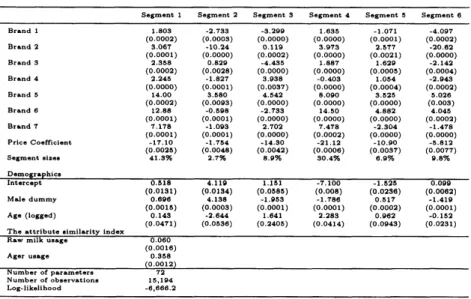
The

parameter estimates of the optimal model with standard errors are presented in Table 2.

All parameters are significant at 1% level.

$\overline{8The\inf ormat\mathring{i}n}$_{sources are as follows:Rawmilk price andcreampriceindexare obtained}fromthedatabaseof “Japan

DalryAssociation”; labor wage infourprefecturesareobtalned from statisticaldepartmentsofcorresponding prefectures;

international sugar pnce is obtained from the database of “Agriculture&Livestock Industries Corporation”;international

oilpriceisobtained from “U.S. EnergyInformationAdministration.”

9Additionally, we constructedand estimated two othermodels, which are a multinomial logit model without state dependence and themodel with lagged brand choicedummyvariable with thesamenumber of segments to compare the

Table 2: Parameterestimatesof theoptimalmodel.

Segment1 Segment2 Segment 3 SegmentSegment 44SegmentSSegmentSegment66 Brand1 1803 $-27S3$ $-S299$ 1635 $-1071$ $\fbox{Error::0x0000}4097$ $(00002)$ (0.0003) $(0$0000$)$ $(00000)$ ($0$OOOI) $(0$0002$)$ Brand2 3067 $-1024$ 01193$97S$ 2.$577$ $-2062$ $(0 0001 ) (0 0000 ) (0 0002 ) (0 0000 ) (0 0021 ) (0 0000 )$ Brand 3 2358 $0829$ $-44S5$ 1 887 $1629$ $-2.142$ $(0$0002$)$ ($O$_.0028) $(0$0000$)$ $(00000)$ (0.0005) $(0$0004$)$ Brand4 2245 $-1827$ 3938 $0403$ 1064 $-2.943$ $(00000) (00OOI) (00OS7) (0 0000 ) (0 0004 ) (0 0002 )$ Brand 5 1400 3580 4.542 8090 3.525 5026 $(0$0002$)$ $(0$0093$)$ $(00000)$ (00000) $(00000)$ $(000S)$ Brand 6 1288 -O.698-2.733 14.50 4.882 4045

$(0$0001$)$ (O. OOOI) (00000) $(00000)$ $(00000)$ (O. 0002)

Br $nd7$ 7.$178$ $-1093$ 27027478-2.304 $\fbox{Error::0x0000}1478$

($O$._{0001) (0.0001) (0.000}$O$₎ $(0$0002$)$ $(O.0000)$ $(0$0000$)$

Price Coefficient $-1710$ $-1754$ $-14$SO $-2112$ $-1090$ $-8812$ $(0002b\rangle (0 0048 ) (0 0042 ) (0 0006 ) (0 0037 ) (0 0077 )$

Segmenteizes 41 S% 2.7% 89% $30$4% $6$9% 9.8%

$\frac{D\cdot\mathring{m}r\bullet hic\epsilon}{}$

Intercept 051841191161 $-7100$ $-1626$ 0099 $(0$0131$)$ ($0$OI34) (0.0585) (0.008) $(0$₀₂₃₆$)$ (0.0062) Male dummy 0.696 4 IS8 $arrow 196S$ $-1786$ $0617$ $-1419$

$(0 0015 ) (0 0003 ) (0 0001 ) (0 0001 ) (0 0002 ) (0 0001 )$

Age(logged) O.$143$ $-2644$ 1641 $228S$ $0962$ -O.152

$(0$0471$)$ $(0$0536$)$ (0.2405) $(0$₀₄₁₄$)$ $(0$0943$)$ $(0$0231$)$

$\frac{Thoattr1but*s1mllarltylndex}{R\cdot wmi1ku\cdot\cdot\zeta e0060}$ $(0 0016 )$

Agerusage $0368$

$\frac{(OO012)}{Numberofparamoters72}$

_{Numberof observations 15,194} ${\rm Log}$_{-likelihood $-6,6662$}

In Table 2, ”Brand” entries represent brand-specific intercepts relative to outside $or\succ$

tions, presented below “Demographics” entry

are

parameters for calculating $SD_{s}$, which

isaparameterofthe attribute similarity index in (2), andpresentedbelow “The attribute

similarity index” entry

are

the estimatesof importance weights fortwo attributes to

cal-culate the attribute similarity

index.10

Because

we

find that using all three attributes

results in anomalies in estimation, we chooseto

remove

“Fat level”’ attribute. Thelarger

number of “Ager usage” relative to “Raw milk usage” suggests that perceived similarity

between brands largely depends onthe type of yogurt (i.e., whether yogurt is hard-type

or plain-type).

Wecalculated how statedependence tendency varies

across

segments by genders using

mean

age. Households in segment 4 and

6

are

found to be variety-seekers and the rest

is almost all inertial. Only segment 2 had opposingsigns for state dependence tendency

dependingongender (malesin this segment exhibit strong inertial tendency whilefemales

exhibit modest variety-seeking tendency). Overall,

we

do notseethe consistent

relation-shipbetween state dependence tendencies and demographic variables. Beingmale affects

theutilityofthe similarbrand topreviously purchasedoneeither positivelyor negatively,

and thesameistrue for age.

$1\fbox{Error::0x0000}We$only present

estimates ofimportance weightsforsegment 1 in Table2. This is because weestimated them with the model without segment and usedthese estimatesfor the models with the greater number of segments. In other words, we assumedperceptions ofsimzlarity between brandswere commonacrosssegmentsasin [4]. This isbecauseestimating themodel without thisassumptionwouldhaveincreased the number ofparameters by 66, and this could have made the estimation unstable.

Table3: Margins (Unit: yen per gram)under eachmodel and game.

Brand1 Brand2 Brand 8 Brand 4 Brand5 Brand 6 Brand 7

$\underline{AveragePrices0451050405lS0480112711280S59}$

Retail margin O051 O.109 O.105 $0104$ 0313 O.187 O.103

$(0 0006 ) (0 0013 ) (0 0031 ) (0 0024 ) (0 0051 ) (00026\rangle (0 0019 )$

$\underline{manufacturerStackelberg}$

Bertrandcompetition $0039$ $0$IOO $0007$ $0125$ 0039 $0115$ $0085$ ($O$.₀₀₀₆₎ $(0$0028$)$ $(0$0044$)$ $(0$0015$)$ $(0$0033$)$ $(0$0014$)$ $(00010\rangle$

Tacit collusion $0048$ $0131$ $0018$ $0147$ $0045$ O119 $0$I07

$(000IO)$ $(0$₀₀₂₃$)$ $(0$0046$)$ $(0$0015$)$ ($O$.0036) $(0$0013$)$ $(0$0021$)$

verticalNash

Bertrand competition 0042 O.084 $0088$ $0084$ 0304 $0182$ $008S$ (O0006) $(0$0002)0002$)$ (O. 0026)0026) $(0$₀₀₁₆$)$ $(0$0050$)$ $(0$0027$)$ ($O$OOII)

5.2 Supply-Side Results

In this subsection, we will present the results of margins, marginal cost and model

comparison. Though the actual calculations proceed in this order,

we

first present the

result of model comparison as it helps the interpretation of the results of margins.

5.2.1 ${\rm Log}$-likelihood for supply-side and Vuongtest statistics

After calculating margins,

we

calculated the $\log$-likelihood for supply-side in (11) and

Vuong test statisticsto compare thefits ofthreemodels and games in thesemodels. We

find that the market is best described by the verticalNash-Bertrandcompetition game.

In addition to forward-looking model, where firms account for the impact of current

price on future profit, we also conducted analysis using static model and myopic model.

The static model is a standard multinomial logit model without state dependence and

the myopic model assumesthat firms account for state dependence in demand (i.e., firms

considerthe effect ofahousehold previousbrandchoice via the attribute similarity index)

but do not account for the future profit associated with current pricing decision. We

compare the Vuong test statistics across models to find that the best-fitting model (the

verticalNash-Bertrandcompetitiongamein forward-looking model) is statisticallybetter

than anyother models and games.

5.2.2 Margins

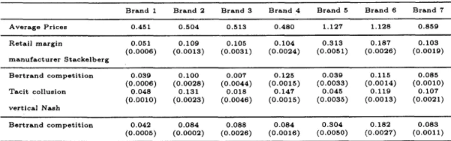
The margins (in yen per gram) of suggested model are presented in Table3. It should

be noted that margins in the vertical Nash-Bertrand competition game in Table 3 are

our best estimate within the employed framework, and those in the other entries are

counter-factual in thesense that, had these sorts ofgamesand perspectives werein play,

First of all, manufacturers’ margins under tacit collusion always exceed those under

Bertrand competition

as

expected. However, for brand 1, 3, 5 and 6, the margins under

manufacturer Stackelberg

are

lower than vertical Nash counterparts in both myopic and

forward-looking models regardless of which game in horizontal interaction is assumed.

Thisisonepiece of evidence thatmanufacturer Stackelberggamebetween manufacturers

and aretailer cannot be justified with data.

Remember that brand3 has

a

distincttaste advantagedue tothe fact that it

uses

only

raw

milk, while brand

5

and

6

are

the yogurt with special lactic-acid bacilli. Therefore

we expect that these brands to command higher margins. As expected, brand 3, 5 and

6 command three largest margins under the vertical Nash-Bertrand competition game

(0.088, 0.304, and

0.182

respectively), whichwe estimate to reflect Japanese yogurt

mar-ket. Meanwhile, brand 3 and 5 havethe least and the second least margins respectively

under the manufacturer Stackelberg-Bertrand competition counter-factual (0.007 and

0.039), whichis another evidence that manufacturer Stackelberg game cannot be justified

with

data.11

These facts and the market being characterized by the vertical Nash-Bertrand

com-petition game jointly imply that differentiating brands by improving its quality enables

manufacturers to charge higher margins relative to the others. However,

we

note that

a retailer also charges the largest and the second largest margins for brand 5 and

6

and

chargesthefourthlargest margin for brand3. In fact, theamount of retailer’smargins

are

higher than manufacturers’ margins for all brands in the vertical Nash-Bertrand

com-petition game

as

shown in Table 3. These facts lead usto the conclusion that a retailer

hasmore power than manufacturers. The decreasing price ofyogurt over thelast decade

is at least partially due to decreasing power of manufacturers relative to the retailer in

addition to competition among manufacturers

as

indicated by

our

result. The existence

of fierce competition among manufacturers makes sense,

as

157yogurt brands existed in

themarket in January

2007

to December 2008.

5.2.3 Marginalcost

Theestimation result for marginal cost of the vertical Nash-Bertrand competition game

of the proposed model is presented in Table$4^{}$ Wefindthat after includingmanufacturer

dummyvariables, all variablesexcept for international oil price have negative coefficients

in the best-fitting game, thus we exclude

them.13

The high values for manufacturers

$\overline{1lThemargim}$

ofBrmd1$md5$ under themanufacturerStackelberg-Bertrand competition gamein forward-looking

modelappear to be thesamein Table 3, but this is because of rounding. The margin ofbrand1 is shghtly larger than that ofbrand5,even though the difference is minimal.

12Resultsforthe other modelscanbe provided upon the request to the author.

13Ifweuseonly labor wage, their coefficients are positive. The effect of labor wageseemsto beabsorbed bymanufacturer

Table4: Marginal cost estimation in forward-looking model.

manufacturerStackelberg Bertrand competition Tacit collusion

$\overline{t\fbox{Error::0x0000}valuop}$

Estimate Std.Err $p$-value Estimate Std Err $t$-value

$\overline{Intercept07420233}3182 0002 \fbox{Error::0x0000}0816 0240 3408 0001$

Manufacturer 2 $0041$ $0026$ $-159S$ $0110$ $-0061$ $0027$ $-2319$ 0021 Manufacturer$3$ $-0026$ $0030$ $\fbox{Error::0x0000}0880$ $0379$ $0031$ $0031$ $-1004$ O316

Manufactur\’er4 0.287 O0221322 $0000$ $0287$ $0022$ 12870000 Manufacturer6 $0346$ $0027$ 13 $0000$ 0335 $0027$ 12 0000 Cream price index 0133O0324137O000O1390033 4192 $0000$

Internationaloilprice $0038$ $0024$ 1546 $0123$ $0037$ O025 1480 0.139 $\frac{Rawm1kprice00030002110402700003\mathring{0}00212780202}{vertica1NashBertrandcompetitionTac\mathfrak{i}tc11u\cdot ion}$ $\frac{Estimat\’{e} StdErrt-va1uep-va1ueEstimateStdErrtva1uep\fbox{Error::0x0000}va1ue}{Intercept0196008224010.01701870.08422250.026}$ Manufacturer$2$ $-0048$ $0021$ $-2280$ O. 023 $0063$ $0021$ 2918 0.004 Manufacturer 3 $0037$ $0021$ 1778 $0076$ $-0044$ $0021$ 2075 $003S$ Manufacturer 4 O.163 00179563 $0000$ 0161 $0018$ 9193 0000 Manufacturer5 0315 $0021$ 1511 $0000$ $0304$ $0021$ 1417 0000

International oil price $0037$ $0018$ 2015 $0044$ $0037$ $0019$ 1967 $0061$

4 and 5

are

consistent with the fact that manufacturer 4 produces brand 5 and 6 and

manufacturer 5 produces brand

7.

5.2.4 The price endogeneity

After estimating $\hat{\xi_{jt}}$

and $\hat{\eta_{jt}}$, wetested the correlation between them using one of

Pear-son’s product moment correlation coefficient test. The test reveals that they

are

signif-icantly correlated and thus prices

are

proven to be endogenously determined, which is

consistent with the general finding in literature.

6

Conclusion

In this paper, weempirically analyzed Japanese yogurt market incorporating consumer

heterogeneity,

consumer

state dependence, forward-looking behavior ofmanufacturersand

aretailer, and priceendogeneity arises from the interaction between unobserved demand

characteristics and prices. Ourdemand-side findingsareconsistent with those of previous

literature; consumers areheterogeneous in their responsiveness tomarketingvariables and

degreesofstate dependence. Onsupply-side, wefindpricesareendogenouslydetermined,

manufacturers engage in Bertrand competition game, manufacturers and a retailer play

vertical Nash game, and they set prices considering their impact on future profit.

We find that brands with differentiating features (brand 3, 5 and 6) do command

higher margins, proving that manufacturers’ efforts are rewarded. However, a retailer

also charges higher margins for these brands and obtains larger split of the profit. We

alsofind that there arerigorous competitions among manufacturers in this marketwhich

competition

was

the

case

in the

U.S.

cerealmarket with largenumberof brands. Finally,

our work adds another evidence to the body of literature in this field of intersection be

tween marketing and neo empirical industrial organization,

as

lack of empirical study is

general

concern

in this

area

[10].

One major limitation of this research is the assumption of a monopolistic retailer

as

retailers

are

likely to compete in reality. In fact, “National Survey of Prices”’ conducted

byStatisticsBureau, Ministry ofInternalAffairsandCommunicationsin Japan indicates

that the average retail prices of yogurt are higher in stores withno competitors around.

Incorporating retail competition in the framework employed in this study would be an

interesting

source

of future research. The other possible direction of future research is

inclusion the effect of store brand. This topic is common in the literature, and widely

investigated in the context such

as

its effect on power balance between manufacturers,

store loyalty and so forth. As state dependence is often neglected in these analysis,

investigating the effect of store brand in the presented frameworkmayprovide

new

insight

to the literature.

Appendix

In appendix$A$, we derivemargins in myopic model. In appendix$B$, we derive margins

in forward-looking model. Wenote that equations to derive margins in static model

are

identicalto those in myopic model.

A

Margins

in

Myopic Model

We start with margins of

a

retailer

as

it will be used in calculating margins of

manu-facturers.

A.1 Margins ofaRetailer

Theprofit function for the monopolisticretailer is defined

as

$\pi_{R}=\sum_{j=1}^{J}(p_{jt}-w_{jt})S_{jt}M$ (12)

where $w_{jt}$ is the wholesale price for brand$j$ at time $t,$ $S_{jt}$ is the market share, and $M$is

Now by partially differentiating (12) with respect to each retail price$p_{jt}$, setting them

zero, and algebraic manipulations, we have

$(\begin{array}{l}p_{1t}-w_{1t}\vdots p_{Jt}-w_{Jt}\end{array})=-\{\begin{array}{lll}\frac{\partial S}{\partial p}u1t \cdots \frac{\partial S}{\partial p}\Delta lt p_{Jt}{}_{\frac{\partial}{\partial}\lrcorner}S_{L} \cdots \frac{\partial}{\partial}s_{Jt}\ovalbox{\tt\small REJECT} p\end{array}\}(\begin{array}{l}S_{1t}\vdots S_{Jt}\end{array})$

.

(13)

Using the notation of [4], we have

$(p_{t}-w_{t})=\Phi_{t}^{-1}S_{t}$ (14)

where $(p_{t}-w_{t})\equiv(p_{1t}-w_{1t}, \cdots,p_{Jt}-w_{Jt})^{T}$ is$J\cross 1$ vectorofretail margins, $\Phi_{t}$ is$J\cross J$

matrix with elements

$\Phi_{jkt}=-\frac{\partial S_{kt}}{\partial p_{jt}}$

for brand$j,$$k=1,$$\cdots,$$J$, and $S_{t}$ is $J\cross 1$ vector$S_{t}=(S_{1t}, \ldots, S_{Jt})^{T}.$

A.2 Margins ofManufacturers

Now wederive margins of manufacturersunder different games. Unlikein theretailer’s

case, the profit function of manufacturers differs depending on which game in horizontal

strategicinteractionis assumed. The profitfunction$\pi_{f}$ofmanufacturer$f$under Bertrand

competition isgiven by

$\pi_{f}=\sum_{j\in J_{j}}(w_{jt}-mc_{jt})S_{jt}M$, (15)

where $J_{f}$ isasubset of brands produced bymanufacturer $f$and$mc_{jt}$ is the marginal cost

of producing brand $j$ at time $t$

.

The manufacturer’s margin from brand $j$ is _{$w_{jt}-mc_{jt}.$}

On the otherhand, the totalprofit function $\pi_{\forall f}$ of collusive manufacturers is given by

$\pi_{\forall f}=\sum_{j=1}^{J}(w_{jt}-mc_{jt})S_{jt}M.$

The first order condition of the profit function in tacit collusion game is

$\frac{\partial\pi_{\forall f}}{\partial w_{lt}}=M[S_{lt}+\sum_{j=1}^{J}[(w_{jt}-mc_{jt})\sum_{k=1}^{J}\frac{\partial S_{jt}}{\partial p_{kt}}\cdot\frac{\partial p_{kt}}{\partial w_{lt}}\Vert=0$ (16)

for$l=1$, .

. .

,$J$

.

By algebraic manipulation, we have

$(\begin{array}{l}w_{1t}-mc_{1t}\vdots w_{Jt}-mc_{Jt}\end{array})=-[\{\begin{array}{ll}\frac{\partial p_{1t}}{\partial w_{1t}},\cdot Z\partial L^{t}\partial w_{1t}\frac{\partial p_{1t}}{\partial wJt},\cdot \dot{\partial}w\partial\ovalbox{\tt\small REJECT}_{\frac{t}{Jt}}\end{array}\}$ $\{\begin{array}{ll}\frac{\partial}{\partial}s_{lt}\lrcorner tp,\cdot {}_{\frac{\partial}{\partial}\lrcorner}S_{1}p_{1t}p_{Jt}{}_{\frac{\partial}{\partial}\lrcorner}S_{A}, \frac{\partial}{\partial p}S_{\ovalbox{\tt\small REJECT},Jt}\end{array}\}]^{-1}(\begin{array}{l}S_{1t}\vdots S_{Jt}\end{array}),$

where the

left

hand side

of

equation (17)

is

$J\cross 1$ vector

of manufacturers’

margins. The

first order condition of profit function in Bertrand competition can be derived similarly.

In equation (17), the terms$S_{jt}$ and $\partial S_{jt}/\partial p_{kt}$canbe directlyobtained from the estimated

demand parameters but $\partial p_{kt}/\partial w_{lt}$ cannot be. Thuswe must infer these terms indirectly,

and the difference between manufacturer Stackelberg and vertical Nash stems from how

these terms

are

specified. We start with the manufacturer Stackelberg-Tacit collusion

game because margins under the other games

can

be derived

as

the special

case

of this

game.

A.2.1 Margins under the manufacturer Stackelberg-Tacit collusion game

To infer$\partial p_{kt}/\partial w_{lt}$,

we

exploitthe firstorder condition of the retail profit function defined

in (12);

$\frac{\partial\pi_{R}}{\partial p_{gt}}=S_{9^{t}}+\sum_{k=1}^{J}[(p_{kt}-w_{kt})\frac{\partial S_{kt}}{\partial p_{gt}}]=0$ (18)

for$g=1$,

. . .

,$J$with themarket size$M$removed. Since aretailer is assumedtomaximize

the category profit, the change inwholesalepriceof one brand would affectall retail prices

in the category. Thuswetotallydifferentiate (18) with respecttoprices$p_{jt},$$j=1$,

. . .

,$J,$

and wholesale price $w_{lt}$ for brand $l$, to obtain, for

some

$g,$

$\sum_{j=1}^{J}[\frac{\partial S_{gt}}{\partial p_{jt}}+\frac{\partial S_{jt}}{\partial p_{gt}}+\sum_{k=1}^{J}(p_{kt}-w_{kt})\frac{\partial^{2}S_{kt}}{\partialp_{jt}\partial p_{gt}}]dp_{jt}-\frac{\partial S_{lt}}{\partial p_{gt}}\cdot dw_{lt}=0.$

(19)

Denoting the terms inside the bracket on the left hand side of equation (19) as $v(g,j)$,

we have theset of$J$equations for

some

$l$

as

$\{\begin{array}{l}\nu(1,1)dp_{1t}+\nu(1,2)dp_{2t}+\cdots+\nu(1, J)dp_{Jt}=\frac{\partial S}{\partial p_{1}}Lt .dw_{lt},.:\nu(J, 1)dp_{1t}+\nu(J, 2)dp_{2t}+\cdots+\nu(J, J)d=_{Jt}\cdot dw_{lt}.\end{array}$ (20)

Defining$G_{g}\equiv(\nu(9,1),$

$\ldots,$$\nu(g, J we$ rewrite $the$expression $in (20)$ inmatrix form and

rearrangeit

as

assuming the inverse of the $J\cross J$matrix $(G_{1}, \ldots, G_{J})^{T}$ exists. Ransposingboth sides of

equation (21) and stacking them vertically for $l=1,$$\cdots,$$J$, we have

$[_{\frac{\partial p_{1t}}{\partial w_{Jt}}..A,IL} \frac{\partial p_{1t}}{\partial w\iota t},\cdot\cdot..,\partial\Delta IL\rangle.\cdot,\partial w_{Jt}\partial]=\{\begin{array}{lll}\frac{\partial}{\partial}s_{1t}\Delta p \cdots -\partial_{t}\partial\frac{S}{p_{J}}t \frac{\partial}{\partial}S\lrcorner tp_{1t} \cdots \frac{\partial}{\partial}S_{\ovalbox{\tt\small REJECT}}p_{Jt}\end{array}\} \cdot(G_{1}^{T}, \cdots, G_{J}^{T})^{-1}$ (22)

Substituting (22) into (17), we have the manufacturers’ margins under the manufacturer

Stackelberg-Tacit collusion game as

$(w_{t}-mc_{t}) = -(\Phi_{t}^{T}G^{-1}\Phi_{t})^{-1}S_{t}$ (23)

where $(w_{t}-mc_{t})=(w_{1t}-mc_{1t}, \cdots, w_{Jt}-mc_{Jt})^{T}$ _and $G=(G_{1}^{T}, \cdots, G_{J}^{T})$

.

A.2.2 Margins under the manufacturer Stackelberg-Bertrand competition game

In Bertrand competition, each manufacturer maximizesthe profit from its ownbrands.

Thus in Bertrand competition, (17) applies only to the brands aparticularmanufacturer

produces. This requires replacement of the third term$\Phi_{t}$ in matrix$(\Phi_{t}^{T}G^{-1}\Phi_{t})^{-1}$ in (23)

with $\Phi_{t}\cdot*\Omega$, where $\cdot*$ denotes element-by-element multiplication, and

$\Omega$ is $J\cross J$matrix

whose $(j, k)$ _elements are indicator functions taking unity if brands$j$ and $k$ are made by

the

same

manufacturer and zero otherwise. Then we have the manufacturers’ margins

under the manufacturer Stackelberg-Bertrand competitiongame

as

$(w_{t}-mc_{t})=-(\Phi_{t}^{T}G^{-1}\Phi_{t}\cdot*\Omega)^{-1}S_{t}$

.

(24)

A.2.3 Margins under theverticalNash-Tacit collusion game

In the vertical Nash game, manufacturers and a retailer move simultaneously. More

specifically, manufacturers set wholesale price expecting a certain level of retail margin

forthe brand;aretailersets its retail margin for each brand basedonits profit maximizing

behavior. Now by assumption, we have the relationship

$\frac{\partial(p_{jt}-w_{jt})}{\partial w_{jt}}=0$

orequivalently

$\frac{\partial p_{jt}}{\partial w_{jt}}=1$ (25)

for all $j=1$ ,

.

.

.

,$J$ since the retail margin of brand $j,$ $p_{jt}-w_{jt}$, is not affected by

Similarly,

since

the retail margin of brand,$p_{jt}-w_{jt}$

,

is not affected by the wholesale price

of the other brands,

we

have

$\frac{\partial(p_{jt}-w_{jt})}{\partial w_{kt}}=0$

orequivalently

$\frac{\partial p_{jt}}{\partial w_{kt}}=0$ (26)

for$j=1$,

. .

.

,$J,$$j\neq k^{14}$ Finally, from(25) _{and (26), the matrix with elements}$\partial p_{jt}/\partial w_{kt}$

on the right-hand side of equation (17) becomes

an

identity matrix and equation (17)

becomes

$(\begin{array}{l}w_{1t}-mc_{1t}\vdots w_{Jt}-mc_{Jt}\end{array})=-\{\begin{array}{lll}\frac{\partial S}{\partial_{P1}}At \cdots \frac{\partial}{\partial}S_{\Delta}p_{1t} \frac{\partial}{\partial}S\lrcorner\iota p_{Jt} \cdots \frac{\partial S}{\partial p}\Delta Jt\end{array}\}(\begin{array}{l}S_{1t}\vdots S_{Jt}\end{array})$

Thus we have manufacturers’ margins under the vertical Nash-Tacit collusion game

as

$(w_{t}-mc_{t})=\Phi_{t}^{-1}S_{t}$ (27)

which is identical to margin of the retailer. This makes

sense

as

the vertical Nash game

assumes

approximately equal power between manufacturers and aretailer [6].

A.2.4 Margins under the vertical Nash-Bertrand competition game

Since the retailer behaves the same independent of whether manufacturers compete

or tacitly collude, the conditions (25) and (26) still hold in the vertical Nash-Bertrand

competitiongame. And by thesamereasoning of themanufacturerStackelberg-Bertrand

competitiongame,

we

havethemanufacturers’ margins under the verticalNash-Bertrand

competition game

as

$(w_{t}-mc_{t})=(\Phi_{t}\cdot*\Omega)^{-1}S_{t}$

.

(28)

$\overline{14We}$

note thattbs behavioralpnncipleof retalerisconsistent with its profit mmmizing behavior,asthepredetermined

retailmargms arestill determined from the first order condition of its profit function

$\frac{\partial\pi R}{\partial p_{gt}}=S_{gt}+\sum_{k=1}^{J}[(p_{kt}-w_{kt})\frac{\partial S_{kt}}{\partial p_{gt}}]=0$

B

Margins

in

Forward-Looking

Model

Here we derive the margins in forward-looking model. We start with the margin of a

retailer.

B.1 Margins of

a

Retailer (Forward-Looking Model)

The objectivefunction ofone-periodforward-lookingretaileris$V_{R}=\pi_{R1}+\delta\pi_{R2}$, where

$\pi_{Rt}$ is a profit function defined in (12) for period$t=1$, 2, and the term

$\delta$

is some

exoge-nously given discount rate. Then the first orderconditions are

$\{\begin{array}{l}\frac{\partial}{\partial}\pi_{k1}AL+\delta\sum^{J_{\frac{\partial}{\partial}n^{\pi}a}.\partial S_{2}}j=1S_{j2}\hat{\partial S_{j1k1}}\frac{\partial}{\partial}\frac{S}{p}L^{1}p.= 0\partial\pi\partial_{Pk2} = 0\end{array}$ (29)

for $k=1$,

.

.

.

,$J$

.

In (29), the first equation corresponds to the first order condition of

thefirst periodprofitfunction and the secondequation correspondsto that of the second

periodprofit. As the first order condition inthe secondperiod is alreadyknown, weonly

concern

for the first equation in (29) in the following derivation. Furthermore, in that

equation, the unknownterms are $\partial\pi_{R2}/\partial S_{j2}$ and $\partial S_{j2}/\partial S_{j1}.$

Clearly, $\partial\pi_{R2}/\partial S_{j2}$ is $(p_{j2}-w_{j2})$

.

To calculate $\partial S_{j2}/\partial S_{j1}$,

we

exploit the following

relationship:

$S_{j2}= \theta_{j2|j1}\cross S_{j1}+\sum_{l=1,l\neq j}^{J}\theta_{j2|l1}\cross S_{l1}$ (30)

where $\theta_{j2|j1}$ is the probability of purchasing brand$j$ in period2given the purchase of the

brand in period 1, and$\theta_{j2|l1}$ isdefinedlikewise withbrand$l$

.

Sincethe market share sums

up to one, the term $S_{l1}$ isrewritten as _{$S_{l1}=(1-S_{11}-\cdots-S_{l-1,1}-S_{l+1,1}-\cdots-S_{J1})$}

for all $l=1$,

.

.

.

,$J,$ $l\neq j$, which includes the term $-S_{j1}$

.

Thus, the partial derivative of

the second termonthe right-hand side of equation (30) with respect to $S_{j1}$ is

$\frac{\partial[\sum_{l=1,l\neq j}^{J}\theta_{j2|l1}\cross S_{l1}]}{\partial S_{j1}}=-\sum_{l=1,l\neq j}^{J}\theta_{j2|l1}$

as $\partial S_{l1}/\partial S_{j1}=-1$ for $l=1$,

. .

.,$J,$ $l\neq j$

.

Thus taking partial derivative of both sides of

(30) with respect to $S_{j1}$,

we

have

$\frac{\partial S_{j2}}{\partial S_{j1}}=\theta_{j2|j1}-\sum_{l=1,l\neq j}^{J}\theta_{j2|l1}$

.

(31)

In the

same

manner as

in the derivation of vector $(p_{t}-w_{t})$, the second term on the

left-hand side ofthe first equation in (29)

can

be expressed by matrix form

as

$\delta\{\begin{array}{lll}\frac{\partial}{\partial}p_{11}S_{\lrcorner\perp} \cdots \frac{\partial S}{\partial p_{l}}\perp 1 \frac{\partial S}{\partial p}LJ1 \cdots \partial S_{1}\vec{\partial_{PJ1}}\end{array}\} \{\begin{array}{lll}\triangle_{1} \cdots 0 0 \cdots \triangle_{J}\end{array}\} (\begin{array}{l}p_{12}-w_{12}\vdots p_{J2}-w_{J2}\end{array})$

where the second matrix is diagonal matrix with diagonal elements $\Delta_{j}$, which

we

will

express

as

$\Delta$

.

Thus

we

havethe margin inthe first period

as

$(\begin{array}{l}p_{1l}-w_{11}\vdots p_{J1}-w_{J1}\end{array})=-\{\begin{array}{lll}\frac{\partial}{\partial}\frac{S}{P1}\perp 1 \cdots \partial S\perp\vec{\partial_{P1l}} -\frac{\partial S}{\partial_{PJ}}\iota 1 \cdots \partial S\perp\vec{\partial_{PJ1}}\end{array}\}$ $(\begin{array}{l}S_{11}\vdots S_{J1}\end{array})-\delta\{\begin{array}{lll}\Delta_{1} \cdots 0 0 \cdots \triangle_{J}\end{array}\}$ $(\begin{array}{l}p_{12}-w_{12}\vdots p_{J2}-w_{J2}\end{array})$

or $(p_{1}-w_{1})=\{\Phi^{T}\}^{-1}S_{1}-\delta\Delta(p_{2}-w_{2})$, assuming the inverse of $\Phi^{T}$ exists. To derive

margins in forward-looking model, wefirst calculate the margins in the myopic

case

from

week 2, and use these margins in calculating margins in forward-looking model starting

from week 1.

B.2 Margins of Manufacturers (Forward-Looking Model)

Thederivationofmargins ofmanufacturersin one-period forward-looking model much

followsthe

case

of the retailer. Here

we

consider the margin in themanufacturerStackelberg-Tacit

collusion game as margins in the other games are special case of those under thisgame.

The objective functionis $V_{M}=\pi_{f1}+\delta\pi_{f2}$ and thefirst orderconditions

are

$\{\begin{array}{l}\frac{\partial\pi f1}{\partial wk1}+\delta\sum^{j}=1\frac{\partial\pi_{f2}}{\partial S_{j2}}.\frac{\partial S}{\partial S}\angle^{2_{-}}j1^{\cdot}\partialS_{1}k1 = 0\frac{\partial\pi_{f2}}{\partial w_{k2}} = 0.\end{array}$ (32)

As

was

the casein (29), the first equation of(32) correspondsto thefirst order condition

of the first period profit function and the second equation corresponds to that of the

secondperiod profit. Clearly, $\partial\pi_{f^{2}}/\partial S_{j2}=(w_{j2}-mc_{j2})$

.

Then the product ofthisterm

and $\partial S_{j1}/\partial w_{k1}$ turns out to be the second termof the first order condition of the profit

functionofmanufacturersin (16), exceptfor the subscript being2insteadof$t$in wholesale

price$w_{j2}$ and marginalcost $mc_{j2}$

.

Then thisproduct term can bewritten in matrixform

as

or

simply $\Phi_{t}^{T}G^{-1}\Phi_{t}(w_{2}-mc_{2})$

.

Thus the second termon the left-hand side of the first

equation of(32) becomes $\delta(\Phi_{t}^{T}G^{-1}\Phi_{t})\Delta(w_{2}-mc_{2})$

.

Then wehave $S_{1}+\Phi_{t}^{T}G^{-1}\Phi_{t}(w_{1}-$

$mc_{1})+\delta(\Phi_{t}^{T}G^{-1}\Phi_{t})\Delta(w_{2}-mc_{2})=0$or$(w_{1}-mc_{1})=-(\Phi_{t}^{T}G^{-1}\Phi_{t})^{-1}S_{1}-\delta\cdot\Delta(w_{2}-mc_{2})$,

assuming the inverse of $\Phi_{t}^{T}G^{-1}\Phi_{t}$ exists. The margins in the other games are derived

similarly

as

we presented in the myopic

case.

References

[1] Steven T Berry. Estimating discrete-choice models of product differentiation. The

RAND Journal

_of

Economics, pages 242-262, 1994.

[2] David Besanko, Jean-PierreDub\’e, and Sachin Gupta. Competitive price

discrimina-tion strategies inaverticalchannel using aggregate retail data. Management Science,

$49(9):1121-1138$, 2003.

[3] DavidBesanko, SachinGupta, andDipak Jain. Logitdemand estimation under

com-petitive pricing behavior: An equilibrium framework. Management Science, $44(11-$

$part-1):1533-1547$, 1998.

[4] Hai Che, K Sudhir, and PBSeetharaman. Bounded rationality in pricing under

state-dependent demand: Do firms look ahead, and if so, how far? Journal

_of

Marketing

Research, pages 434-449, 2007.

[5] Pradeep K Chintagunta. Investigating category pricing behavior at a retail chain.

Journal

_of

Marketing Research, $39(2):141-154$, 2002.

[6] S Chan Choi. Price competition in a channel structure with a common retailer.

Marketing Science, $10(4):271-296$, 1991.

[7] Michaela Draganska and DipakCJain. Consumerpreferences and product-line

pric-ing strategies: An empirical analysis. Marketpric-ing science, $25(2):164-174$,

2006.

[8] Michaela Draganska and Daniel Klapper. Retail environment andmanufacturer

com-petitive intensity. Journal

_of

Retailing, $83(2):183-198$, 2007.

[9] Dan Horsky and Paul Nelson. New brand positioning and pricing in anoligopolistic

market. Marketing Science, 11(2):133-153, 1992.

[10] Vrinda Kadiyali, K Sudhir, and Vithala R Rao. Structural analysis of competitive

behavior: Newempiricalindustrial organization methods in marketing. International

[11] Wagner A. Kamakura and Gary J. Russell. Aprobabilistic choice model for market

segmentationandelasticitystructure. Journal

_of

Marketing Research,$26(4):379-390.,$

1989.

[12] James M. Lattin. A model of balanced choice behavior. Marketing Science, $6(1):48-$

65., 1987.

[13] Sergio Meza and K Sudhir. Do private labels

increase

retailer bargaining power?

Quantitative Marketing and Economics, $8(3):333-363$,

2010.

[14] Aviv Nevo. Measuringmarket power in the ready-to-eat cereal industry.

Economet-rica, $69(2):307-342$, 2001.

[15] Margaret E Slade. Product rivalry with multiple strategic weapons: An analysis of

price and advertising competition. Journal

_of

Economics

&

Management Strategy,

$4(3):445-476$,

1995.

[16] S Sriramand VrindaKadiyali. Empirical investigation of channelreactionstobrand

introductions. InternationalJournal

_of

Research in Marketing, $26(4):345-355$, 2009.

[17] K Sudhir. Structural analysis ofmanufacturer pricing in the presence of

a

strategic

retailer. Marketing Science, $20(3):244-264$,

2001.

[18] J Miguel Villas-Boas and Russell S Winer. Endogeneity in brand choice models.

Management Science, $45(10):1324-1338$, 1999.

[19] J Miguel Villas-Boas and Ying Zhao. Retailer, manufacturers, and individual

con-sumers:

Modelingthe supplyside in the ketchup marketplace. Journal

_of

Marketing

Research, pages 83-95,

2005.

[20] Sha Yang, Yuxin Chen, and Greg M Allenby. Bayesian analysis of simultaneous

demand and supply. Quantitative Marketing and Economics, $1(3):251-275$, 2003.

Graduate School of Systems and Information

DivisionofPolicy and Planning Sciences

University of Tsukuba

Tsukuba

305-8573

JAPAN

$E-$-mail address: _{[email protected]}

$E-$-mail address: _{[email protected]}

$\ovalbox{\tt\small REJECT}\grave{y}oe\star g\backslash y$ス$\overline{\tau}$ム

rex

エ$\not\cong\Re_{J\iota}^{*}\#t$ $\mathfrak{G}\#$ $x)_{\backslash }$