内部波ビームの3次元的安定性 (非線形波動現象の数理と応用)

内部波ビームの

3

次元的安定性

神戸大学 (Kobe University) 片岡 武 (Takeshi Kataoka)

Massachusetts Institute of Technology Triantaphyllos R. Akylas

要旨 一様な密度成層流体中を伝播する内部波ビームの 3 次元撹乱に対する線形安 定性を取り扱った。 具体的には，撹乱の波長がビームの幅に比べて十分長い場 合を仮定し，漸近理論を駆使して Euler方程式系を基に変調安定性を調べた。 その結果，一方向のみにエネルギーを伝える進行波ビームは，振幅がある値を 超えると変調不安定となり，両方向にエネルギーを伝える定在波ビームは，任 意の振幅において変調不安定となることが分かった。

1.

緒言

In

an

inviscid, incompressible, unifonnly stratified fluid ofconstant Brunt-V\"ais\"al\"afrequency $N_{0}$,

a

plane intemal

wave

has the

wave

frequency $\omega$ which is

a

function only of the angle $\theta$ between the

wavenumberdirection and thevertical[l]:

$\omega=N_{0}\sin\theta$

.

(1.1)

Theinternalwavebeaminvolvesplanewaveswithvariouswavenumbers $l$ foracertain fixedangle $\theta,$

and thebeam is localized inthe wavenumber direction. Such localization is possible because intemal

waves

essentially propagate perpendicular tothe

wave

crest.

Intemal

wave

beams

can

be readily produced from

a

two-dimensional oscillating

_source

of

a

given

frequency $\omega_{0}(<N_{0})$

.

The inducedsteadybeampattemconsists of fourstraightlinesstretchingfrom the

source

withthe angles $\pm\cos^{-1}(\omega_{0}/N_{0})$ tothevertical. Thiswell-knownpattemiscalled ‘StAndrew’s

Cross’, andwas first verified experimentally by Mowbray & Rarity[2] usingvibration ofa horizontal

cylinder

as

an

oscillating

source.

Inthepresent study,

we

examinethe linearstabilityofthese internal

wave

beamsto long-wavelength

three-dimensionalperturbations. The stabilityof the internal

wave

beam

was

treatedin thepast only by

Tabaei andAkylas[3], andtheyfoundthat thewavebeam istwo-dimensionally stable.Herewe examine

the stability to three-dimensional perturbations, and found that they are, in fact, three-dimensionally

unstable iftheir amplitude exceeds some threshold value for progressive beams and unstable for any

amplitudeforpurely standingbeams.Thisreportis based

on

Kataoka andAkylas[4].

2.

基礎方程式

Consider three-dimensional internal

wave

disturbances in

an

inviscid, incompressible, uniformly

stratified Boussinesq fluid of constant Brunt-V\"ais\"al\"a frequency $N_{0}$

.

Forthe purpose ofstudying the

stability of

an

intemal

wave

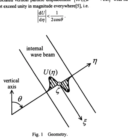
beam, it is convenientto work with the spatial coordinates $(\xi,\eta,\zeta)$, the

along-beam, across-beam and horizontal transverse directions, respectively (Fig. 1). We

use

dimensionless variables throughout, employing the

same

scalings

as

in Tabaei

&

Akylas[3] (with the

beam width

as

characteristic length, $1/N_{0}$

as

time scale, and

a

typicalvalue ofthebackgrounddensity).

$\nabla\cdot u=0$, (2.la)

$\rho_{l}+u\cdot\nabla\rho=-u\sin\theta+v\cos\theta$, (2.lb) $u_{t}+u\cdot\nabla\rho=-p_{\xi}+\rho\sin\theta$, (2.lc) $v_{t}+u\cdot\nabla v=-p_{\eta}-\rho\cos\theta$ , (2.ld) $w_{t}+u\cdot\nabla w=-p_{\zeta}$ , (2.le)

where $\theta$ is

an

angle between the

$\eta$ axis and the vertical,

$t$ is the time, and $\rho$ and $p$

are

the

densityand

pressure

perturbations fromthe backgroundstate,respectively, andthe subscripts $t,$ $\xi,$ $\eta$

and $\zeta$ denote partialdifferentiationwithrespect tothesevariables.

Equations(2.1)have the$fol[oWil$

$\{$

$ng$exact solution representing fmite-amplitude internal

wave

beam

$u=u_{0}(t,\eta)\equiv\{U(\eta)e^{-i\sin\theta t}+c.c.\},$

$v=w=0,$

$\rho=\rho_{0}(t,\eta)\equiv\vdash iU(\eta)e^{-isi\theta l}+c.c.\}$, (2.2) $p=p_{0}(t,\eta)\equiv\{$

icos$\theta\int U(\eta’)d\eta’e^{-i\sin\theta t}+$

c.c.

$\},$

where $U(\eta)$ is

a

given arbitrary function of $\eta$ which decays rapidly

as

$\etaarrow\pm\infty$ and

c.c.

denotes

complex conjugate. In the present study

we

exclude the limiting

cases

of $\thetaarrow 0$ and $\pi/2$ for which

the internal

wave

beam approaches

a

horizontal steady shear flow

or

becomes nearly vertical with frequency closetotheBnmt-V\"ais\"al\"afrequency.Thus,

we

put

$0< \theta<\frac{\pi}{2}$

.

(2.3)

Moreover, in orderto avoid density inversions

so

that the internal

wave

beam (2.6) is statically stable,

the derivative of the associated vertical particle displacement $\{iU(\eta)e^{-i\sin\theta t}+C\mathcal{L}.\}$ with respect to the vertical directionmust notexceed unityinmagnitudeeverywhere[5],i.e.

$| \frac{dU}{d\eta}|<\frac{1}{2\cos\theta}$

.

(2.4)

We examine the linear stability of the above statically stable intemal

wave

beam $(2.2)-(2.4)$ to

three-dimensionalperturbations. Tothisend,employingFloquettheory,

we

write

$\{\begin{array}{l}uvw\rho p\end{array}\}=\{\begin{array}{l}u_{0}(t,\eta)00\rho_{0}(t,\eta)p_{0}(t,\eta)\end{array}\}+\{\begin{array}{l}\hat{u}(t,\eta)\hat{v}(t,\eta)\hat{w}(t,\eta)\hat{\rho}(t,\eta)\hat{p}(t,\eta)\end{array}\}\exp[\sigma t+i$ ($k$

\’e

_$+m\zeta$)$]$, (2.5)

where $(\hat{u},\hat{v},\hat{w},\hat{\rho},\hat{p})$

are

unknown functions of $t$ and

$\eta$ which

are

periodic in $t$ with the

same

period $2\pi/\sin\theta$

as

that of the internal

wave

_beam, $\sigma$ is

an

unknown complex constant, and $k$ and $m$

are

given real constants. Substituting(2.5)into(2.1)andlinearizing withrespecttotheperturbations,

wehave the followingsetofequations for $(\hat{u},\hat{v},\hat{w},\hat{\rho},\hat{p})$:

$ik\hat{u}+\frac{\partial\hat{v}}{\partial\eta}+im\hat{w}=0$ , (2.6a)

$\frac{\partial\hat{\rho}}{\partial t}+\sin\theta\hat{u}+(\frac{\partial\rho_{0}}{\partial\eta}-\cos\theta)\hat{v}=-(\sigma+iku_{0})\hat{\rho}$, (2.6b)

$\frac{\partial\hat{u}}{\partial t}-\sin\theta\hat{\rho}+\frac{\partial u_{0}}{\partial\eta}\hat{v}=-[i\ovalbox{\tt\small REJECT}^{\wedge}+(\sigma+iku_{0})\hat{u}]$, (2.6c)

$\frac{\partial\hat{v}}{\partial t}+\cos\theta\hat{\rho}+\frac{\partial\hat{p}}{\partial\eta}=-(\sigma+iku_{0})\hat{v}$, (2.6d)

$\frac{b\hat{v}}{\partial t}+im\hat{p}=-(\sigma+iku_{0})\hat{w}$

.

(2.6e)

Inadditiontobeing periodicin $t$ with period $2\pi/\sin\theta,$

$( \hat{u},\hat{v},\hat{w},\hat{\rho},\hat{p})(t)=(\hat{u},\hat{v},\hat{w},\hat{\rho},\hat{p})(t+\frac{2\pi}{\sin\theta})$, (2.7) the perturbationsmustalso decayin $\eta,$

$(\hat{u},\hat{v},\hat{w},\hat{\rho},\hat{p})arrow 0$

as

$\etaarrow\pm\infty$

.

(2.8) The above set of equations $(2.6)-(2.8)$ constitutes an eigenvalue problem, $\sigma$ being the eigenvalue

parameter. When there is

a

solution $(\hat{u},\hat{v},\hat{w},\hat{\rho},\hat{p})$ with $\sigma$ having

a

positive real part, the

corresponding internal

wave

beam is linearly unstable. Sincea solution for _$k<0(m<0)$ is obtained

fromthatfor $k>0(m>0)$by $(\hat{u},\hat{v},\hat{\rho},u_{0},\rho_{0},\eta)arrow(-\hat{u},-\hat{v},-\hat{\rho},-u_{0},-\rho_{0},-\eta)(\hat{w}arrow-\hat{w})$,

we

set

$k>0,$ $m\succ 0$

.

(2.9)

3.

漸近解析

$(k\sim m^{3/2}<<1)$

Assuming

now

that theperturbation islong inthe $\xi$ and $\zeta$ directions,thatis, $k$ and _$m$ in (2.9)

are

small,

$k=\epsilon^{3}\kappa,$ $m=\epsilon^{2}$, (3.1) where $\epsilon$ is

a

small

Positive

Parameter and $\kappa$ is

a Positive

$O(1)$ constant,

we

seek

an

asymptotic

solution of$(2.6)-(2.8)$for small $0<\epsilon<<1.$

3.1.

Inner solution

Putting aside the decaying boundaly condition (2.8),

we

seek

a

solution of (2.6) which satisfies the

periodicitycondition(2.7)in $t$ andvariesby _$O(1)$ in

$\{\begin{array}{l}\hat{u}=\hat{u}^{(0)}+\epsilon\hat{u}^{(1)}+\cdots,\hat{v}=\epsilon^{3}\hat{v}^{(3)}+\epsilon^{4}\hat{v}^{(4)}+\cdots,\hat{w}=\epsilon^{2}\hat{w}^{(2)}+\epsilon^{3}\hat{w}^{(3)}+\cdots,\hat{\rho}=\hat{\rho}^{(0)}+\epsilon\hat{\rho}^{(1)}+\cdots,\hat{p}=\hat{p}^{(0)}+\epsilon\hat{p}^{(1)}+\cdots,\sigma=\epsilon^{3}\sigma^{(3)} +\epsilon^{s}\sigma^{(5)}+\cdots,\end{array}$ (3.2)

Substituting (3.1) and (3.2) into (2.6) and collecting the same-order terms in $\epsilon$,

we

obtain

a

series of

equations for $(\hat{u}^{(n)},\hat{v}^{(n+3)},\hat{w}^{(n+2)},\hat{\rho}^{(n)},\hat{p}^{(n)})(n=0,1,2,\cdots)$

:

$i\kappa\hat{u}^{(n)}+\frac{\partial\hat{v}^{(n+3)}}{\partial\eta}=F^{(n)}$, (3.3a) $\underline{\partial\hat{\rho}^{(n)_{+\sin\theta\hat{u}^{(n)}}}}=G^{(n)}$ , (3.3b) $\partial t$ $\partial\hat{u}^{(n)}$ $\overline{\partial t}-\sin\theta\hat{\rho}^{(n)}=H^{(n)}$, (3.3c) $\underline{\partial\hat{p}^{(\hslash)_{+\cos\theta\hat{\rho}^{(n)}}}}=I^{(n)}$ , (3.3d) $\partial\eta$ $\partial\hat{w}^{(n+2)}$ $-+i\hat{p}^{(n)}=J^{(n)}$_{, (3.3e)} $\partial t$

wherethe terms

on

theright-hand sides

are

inhomogeneous terms andgivenby

$F^{(0)}=G^{(0)}=H^{(0)}=I^{(0)}=J^{(0)}=0(n=0)$ _(3.4a)

$\{\begin{array}{l}F^{(n)}=-i\hat{w}^{(n+1)}G^{(n)}=\hat{v}^{(n)}-(\sigma^{(3)}+in\ell_{0})\hat{\rho}^{(n-3)}H^{(n)}=\frac{\partial u_{0}}{\partial\eta}\hat{v}^{(n)}-i\hat{\varphi}^{(n- 3)}-(\sigma^{(3)}+in\ell_{0})\hat{u}^{(n-3)}(n=3,4)I^{(n)}=\frac{\partial\hat{v}^{(n)}}{\partial t}J^{(n)}=\triangleleft\sigma^{(3)}+ixu_{0})\hat{w}^{(n- 1)}\end{array}F^{(n)}=-i\hat{w}^{(n+1)}, G^{(n)}=H^{(n)}=I^{(n)}=J^{(n)}=0(n=1,2) ,(3.4c)(3.4b)$

For $n=0$_, equations _(3.3)

are

_{homogeneous and have} the following nontrivial solution _{that satisfies}

the periodicity condition(2.7)

$\{\begin{array}{l}\hat{u}^{(0)}\hat{v}^{(3)}\hat{w}^{(2)}\hat{\rho}^{(0)}\hat{p}^{(0)}\end{array}\}=\{\begin{array}{l}\frac{0}{V}(3)\overline{W}^{(2)}00\end{array}\}+\{\begin{array}{l}\hat{U}_{-}^{(0)}\int\hat{U}_{-}^{(0)}d\eta’\hat{V}^{(3)}-i\hat{U}_{-}^{(0)}icot\theta\int\hat{U}_{-}^{(0)}dicos\theta\eta’\end{array}\}e^{-i\sin\theta t}+\{\begin{array}{l}\hat{U}_{+}^{(0)}\hat{V}_{+}^{(3)}icot\thetai\hat{U}_{+}^{(0)}\int-icos\theta\hat{U}_{+}^{(0)}d\eta’\int\hat{U}_{+}^{(0)}d\eta’\end{array}\}e^{is\dot{m}\theta t}$, (3.5)

where $\overline{V}^{(3)}$ isconstant

and

Here $\hat{U}_{\pm}^{(0)}(\eta)$ and $\overline{W}^{(2)}(\eta)$

are

as yetundetermined functions of

$\eta$: Capital-letter variables withthe

hat and subscript $\pm$

are

the complexamplitudes of components proportionalto $\sim e^{\pm i\sin\theta t}$ that have the

same

frequency

as

the underlying beam, and variables with the overbar denotemean-flow components

(which

are

independent of $t$); $\overline{V}^{(3)}$ and $\overline{W}^{(2)}$

, in particular, represent $O(\epsilon^{3})$ and $O(\epsilon^{2})$

mean

flows in the across-beam $(\eta)$ and the transverse $(\zeta)$ directions, respectively. The higher hamonic

components$(\sim e^{f2i\sin\theta/}, e^{\pm 3is\dot{m}\theta t},\cdots)$ do notappearatthis level.

For $n\geq 1$, the equations (3.3)

are

inhomogeneous, and the inhomogeneous terms $G^{(n)},$ $H^{(n)},$ $I^{(n)}$

and $J^{(n)}$ on the right-hand sides of_(3.3) must satisfy the following solvability conditions to have a solution

$J^{2\pi/\sin\theta}e^{\pm i\sin\theta t}(\pm iG^{(n)}+H^{(n)})dt=0$, (3.7a)

$J^{2\pi/s\dot{m}\theta}[i(\cot\theta H^{(n)}+I^{(n)})-\frac{\partial J^{(n)}}{\partial\eta}]1t=0$

.

(3.7b)

For $n=1$ and 2, the solvability conditions (3.6)

are

identically satisfied, and

a

solution of (3.3)

satisfying(2.7)becomes the

same

form

as

(3.5) with the numbers intheparentheses, atany superscripts

being added by $n$ and

$\overline{V}^{(n+3)}=-i\int\overline{W}^{(n+1)}d\eta’$ , (3.8a) $\hat{V}_{\pm}^{(n+3)}=-i\kappa\int\hat{U}_{\pm}^{(n)}d\eta’+\cot\theta\int\int’\hat{U}_{\pm}^{(n-1)}d\eta^{n}d\eta’$, (3.8b)

$(n=1,2)$

.

For $n=3$ and 4, the solvability conditions (3.7) become the following six equations for

$(\hat{U}_{-}^{(0)},\hat{U}_{+}^{(0)},\overline{W}^{(2)},\hat{U}_{-}^{(1)},\hat{U}_{+}^{(1)},\overline{W}^{(3)})$

:

$\sigma^{(3)}\hat{U}_{-}^{(0)}=\kappa\cos\theta\int\hat{U}_{-}^{(0)}d\eta’-\frac{dU}{d\eta}\overline{V}^{(3)}$ , (3.9a)

$\sigma^{(3)}\hat{U}_{+}^{(0)}=-\kappa\cos\theta\int\hat{U}_{+}^{(0)}d\eta’-\frac{dU^{*}}{d\eta}\overline{V}^{(3)}$, (3.9b)

$\sigma^{(3)}\frac{d\overline{W}^{(2)}}{d\eta}=2\kappa\cot\theta(\frac{dU}{d\eta}\int\hat{U}_{-}^{(0)}d\eta’+\frac{dU}{d\eta}\int\hat{U}_{+}^{(0)}d\eta’)$ , (3.9c)

$\sigma^{(3)}\hat{U}_{-}^{(1)}=\cos\theta(\kappa\int\hat{U}_{-}^{(1)}d\eta’+\frac{i}{2}$

cote

$\int\int’\hat{U}_{-}^{(0)}d\eta^{n}d\eta’)+i\frac{dU}{d\eta}\int\overline{W}^{(2)}d\eta’$, (3.9d) $\sigma^{(3)}\hat{U}_{+}^{(1)}=-\cos\theta(\kappa\int\hat{U}_{+}^{(1)}d\eta’+\frac{i}{2}\cot\theta\int\int’\hat{U}_{+}^{(0)}d\eta^{n}d\eta’)+i\frac{dU^{*}}{d\eta}\int\overline{W}^{(2)}d\eta’$, (3.9e)

$\sigma^{(3)}\frac{d\overline{W}^{(3)}}{d\eta}=2\cot\theta[\frac{dU^{r}}{d\eta}(\kappa\int\hat{U}_{-}^{(1)}d\eta’+\frac{i}{2}\cot\theta\int\int’\hat{U}_{-}^{(0)}d\eta^{n}d\eta’)$

(3.9f)

$+ \frac{dU}{d\eta}(\kappa\int\hat{U}_{+}^{(1)}d\eta’+\frac{i}{2}\cot\theta\int\int’\hat{U}_{+}^{(0)}d\eta^{n}d\eta’)]$

where the asterisk denotes complex conjugate. These equations for the amplitudes, $\hat{U}_{\pm}^{(0)}(\eta)$ and

$\hat{U}_{\pm}^{(1)}(\eta)$, ofthe primary hannonic perturbation and the induced transverse

mean

flow, $\overline{W}^{(2)}(\eta)$ and $\overline{W}^{(3)}(\eta)$,mustbesupplemented withsuitableboundaryconditions. Specifically,

$\int\int^{l}\hat{U}_{-}^{(0)}d\eta^{n}d\eta’arrow 0, \int\int’\hat{U}_{+}^{(0)}d\eta^{\hslash}d\eta’arrow 0, \int\hat{U}_{-}^{(1)}d\eta’arrow 0, \int\hat{U}_{+}^{(1)}d\eta’arrow 0$ , (3.10)

where matchingwith theouter

solution

(3.13)obtained

in Section 3.2 is

alreadytaken

into

account.

The conditions(3.9)

ensure

that the flow field associated withtheprimary-hannonic perturbation,

as

well

as

the $0(\epsilon^{2})$ transverse

mean

flow component vanishes far away from the beam. The induced

mean

flowat $O(\epsilon^{3})$, however,does notremainlocallyconfined in thevicinityof the beam:

$( \hat{u},\hat{v},\hat{w})arrow\epsilon^{3}\overline{V}^{(3)}(\cot\theta, 1, \frac{\mp i}{\sin\theta}) (\etaarrow\pm\infty)$, (3.11) where $\overline{V}^{(3)}$ is constant. In order to construct

an

overall solution of $(2.6)-(2.7)$ that satisfies the

decaying condition(2.8) in $\eta$ ,

we

must seek

an

outer solution which decays slowly in $\eta$ atinfinity

andisconnectedto(3.11)intheinnerlimit.

3.2.

Outer solution

Introducing

a

reducedcoordinate

$Y=\epsilon^{2}\eta$, (3.12)

we

look for

a

solution which varies by $O(1)$ in $Y$ and is independent of $t$ (mean flow) of the

followingorders

$\hat{u}=\epsilon^{3}\hat{u}_{0}(Y) , \hat{v}=\epsilon^{3}\hat{v}_{0}(Y) , \hat{w}=\epsilon^{3}\hat{w}_{o}(Y) , \hat{\rho}=\epsilon^{6}\hat{\rho}_{0}(Y) , \hat{p}=\epsilon^{4}p_{0}(Y)$

.

(3.13) The orders of (3.13)

are

determined by (3.11) and balance of terms in (2.6) noting that $u_{0},\rho_{0}arrow 0$ $(|\eta|arrow\infty)$

.

Substituting (3.1), $(3.12)-(3.13)$ and $\sigma=\epsilon^{3}\sigma^{(3)}$

into

(2.6) and collecting the same-order

termsin $\epsilon$ ofeach equation,

we

obtain

$\epsilon^{2}x$

Fig. 2 Streamlines of the

mean

flow described by theouter solution (3.15) (with (2.5)). The abscissa $\epsilon^{2}x[=\epsilon^{2}(\xi\cos\theta+\eta\sin e)]$ is the horizontal direction perpendicular to the other horizontal transverse $\epsilon^{2}\zeta$ direction (the ordinate) along the beam positioned at $x=0$

.

Streamlines for

$\{\frac{d\hat{v}_{o}}{\sin\theta dY}+i\hat{w}_{O}=0(3)n^{\hat{u}_{0}-\cos\theta\hat{v}_{O}=0\prime},$

,

(3.14)

Theseequations have

a

solutionwhich decays

as

$|Y|arrow\infty$ andisconnected to(3.11)at _$Y=0$

$\{\begin{array}{l}\hat{u}_{O}\hat{v}_{o}\hat{w}_{O}\hat{\rho}_{O}\hat{p}_{0}\end{array}\}=\{\begin{array}{l}cot\thetal-i/sin\theta\sigma^{(3)}cos\theta/sin^{2}\theta\sigma^{(3)}/s\dot{m}\theta\end{array}\}\overline{V}^{(3)}\exp(-\frac{Y}{\sin\theta})$ for $Y>0$, (3.15a)

$\{\begin{array}{l}\hat{u}_{0}\hat{v}_{O}\hat{w}_{O}\hat{\rho}_{O}\hat{p}_{o}\end{array}\}=\{\begin{array}{l}cot\thetali/sin\theta\sigma^{(3)}cos\theta/sin^{2}\theta-\sigma^{(3)}/sin\theta\end{array}\}\overline{V}^{(3)}\exp(\frac{Y}{\sin\theta})$ for $Y<0$, (3.15b)

where $\overline{V}^{(3)}$

isconstant. The flowdescribed by (3.15)ispurelyhorizontalbecause $\hat{u}_{O}/\hat{v}_{o}=\cot\theta$,and it formsasingle circulating flow which traverses the beam because $\overline{V}^{(3)}$ is

constant(figure2).

Thus, wehave constructed

an

overall solution of$(2.6)-(2.7)$ _{whichsatisfies the decaying condition}

(2.8) _{under the supposition that there is}

_a

_solution $(\hat{U}_{-}^{(0)},\hat{U}_{+}^{(0)},\overline{W}^{(2)},\hat{U}_{-}^{(1)},\hat{U}_{+}^{(1)},\overline{W}^{(3)})$ of the eigenvalue

problem $(3.9)-(3.10)$

.

If the eigenvalue problem $(3.9)-(3.10)$ has

a

solution whose eigenvalue $\sigma^{(3)}$

has

a

positivereal part, the underlyingbeamisunstable. Itspossibility isexplored numericallyin Section

4.

4.

$($

3.

$9)-(3.10)$

の数値解

4.1. Renormalization

Welet

$\psi_{\pm}=\int\int’\hat{U}_{\pm}^{(0)}d\eta^{\nu}d\eta’, \psi_{S\pm}=\int\hat{U}_{\pm}^{(1)}d\eta’, \varphi=arrow\tan\theta\int\overline{W}^{(2)}d\eta’, \varphi_{S}=-i\tan\theta\overline{W}^{(3)},$

(4.1)

$V= \tan\theta\overline{V}^{(3)}, \tilde{\kappa}=2\tan\theta\kappa, \tilde{\sigma}=\frac{2\sin\theta}{\cos^{2}\theta}\sigma^{(3)}, \tilde{U}=\frac{2}{\cos\theta}U,$

andobtain

a

renormalizedversionof theeigenvalue problem$(3.9)-(3.10)$

:

$\tilde{\sigma}\frac{d^{2}\psi_{-}}{d\eta^{2}}=\tilde{\kappa}\frac{d\psi_{-}}{d\eta}-\frac{d\tilde{U}}{d\eta}V$,

(4.2a)

$\tilde{\sigma}\frac{d^{2}\psi_{+}}{d\eta^{2}}=-\tilde{\kappa}\frac{d\psi_{+}}{d\eta}-\frac{d\tilde{U}^{*}}{d\eta}V$, (4.2b)

$\tilde{\sigma}\frac{d\psi_{S-}}{d\eta}=\tilde{\kappa}\psi_{S-}+i\psi_{-}-\frac{d\tilde{U}}{d\eta}\varphi$ , (4.2d)

$\tilde{\sigma}\frac{d\psi_{s+}}{d\eta}=-(\tilde{\kappa}\psi_{S+}+i\psi_{+})-\frac{d\tilde{U}}{d\eta}\varphi$ , (4.2e)

$\tilde{\sigma}\frac{d\varphi_{S}}{d\eta}=-i[\frac{d\tilde{U}}{d\eta}(\tilde{\kappa}\psi_{S-}+i_{\psi_{-}})+\frac{d\tilde{U}}{d\eta}(\tilde{\kappa}\psi_{S+}+i_{\psi_{+}})]$, (4.2f)

with

$\psi_{-}arrow 0, \psi_{+}arrow 0, \frac{d\varphi}{d\eta}arrow 0, \psi_{S-}arrow 0, \psi_{S+}arrow 0, \varphi_{S}arrow\frac{\mp V}{\sin\theta}(\etaarrow\pm\infty)$

.

(4.3)

Equations $(4.2)-(4.3)$ _{constitute the} eigenvalue problem for $(\psi_{-},\psi_{+},\varphi, \psi_{S-},\psi_{s+},\varphi_{S})$, with $\tilde{\sigma}$

being

theeigenvalueparameter.Wesolvethis problem numerically.

The underlying beam profile $\tilde{U}(\eta)$ is chosen to be the

same

Gaussian streamfimction profiles

as

Tabaeietal.[5],

$\tilde{U}(\eta)=\{\begin{array}{ll}U_{0}\zeta A(l)e^{il\eta}dl (proyessive beams), (4.4a)\frac{U_{0}}{2}[A(l)e^{il\eta}dl=-2U_{0}\eta e^{-2\eta^{2}} (standing beams), (4.4b)\end{array}$

where $U_{0}$ is

a

positive parameterand $A(l)=ile^{-l^{l}/8}/\sqrt{8\pi}$

.

Progressive beams describeuni-directional

beams which involveplane

waves

with wavenumbers $l$ ofthe

same

_$sign$only, whereas standingbeams

includethose of both signs. The profile $\tilde{U}(\eta)/U_{0}$

is

shown

in

figure

3.

Statically stablecondition(2.4)

becomes

$U_{0}< \frac{1}{2\cos^{2}\theta}$

.

(4.5)

The intemal wave beams (4.4)

_are

statically stable for any $\theta$ if _{$U_{0}<0.5$}

.

Even for the greater

amplitudes, they

are

statically stable depending

on

the value of $\theta$

.

In what follows,

we

present the

stability results for progressive beamsin Section 4.2 and standing beams in Section 4.3. Fornumerical

methodto solve $(4.2)-(4.3)$,

we

use

the finite-difference method for discretization and

a

standard$QZ$

algorithm for the eigenvaluesolver[6].The parameters of$(4.2)-(4.3)$

are

$\theta,\tilde{\kappa}$ and _{$U_{0}.$} 1 0.5 $\frac{\tilde{U}(\eta)}{U_{0}}0$ $-0.5$ $-1_{-6}$ $-4 -2$ $0$ 2 4 6 $\eta$

Fig.3 Profiles $\tilde{U}(\eta)/U_{0}$ of theprogressive beam(4.4a) (solidline: real part, dashedline: imaginary

4.2. Progressive beams

Computed eigenvalues $\tilde{\sigma}$

with

a

positive real part

versus

$\tilde{\kappa}$

are

plottedinfigure4for $\theta=\pi/6$ and

$\pi/3$

.

Amplitudes of the underlying_beams

are

_chosento

be $U_{0}=0.35,0.5$ and0.65 (thesebeams

are

all

statically stable according to (4.5)$)$

.

Figure $4(a)$ shows that progressive beams

are

unstable for

$U_{0}\geq 0.35$, and according to

our

numerical results, the critical amplitude of the instability is about

$U_{0}=0.3.$

Figure4 also shows that the growth rate ${\rm Re}[\tilde{\sigma}]$,which is

an

increasing functionof $\tilde{\kappa}$

for small $\tilde{\kappa},$

reaches

a

peak at

some

finite $\tilde{\kappa}$

and fmally falls to

zero

at the higher $\tilde{\kappa}$

.

Thus, the instability is

three-dimensional(or oblique).The stability of theinternal

wave

beam

was

first examined byTabaeiand

Akylas[3] to longitudinal (two-dimensional)perturbation which corresponds to $\tilde{\kappa}arrow\infty$ inthe

present

notation,andfound

no

instability. Theirresultisconsistent with

our

result.

The

imaginary

part ${\rm Im}[\tilde{\sigma}]$ ofthe above complex eigenvalues isplotted

in figure$4(b)$

.

It is always

one-signed (negative) and the magnitude

grows

linearly in $\tilde{\kappa}$

with almost the

same

gradient for all

cases.

$\tilde{\kappa} \tilde{\kappa}$

Fig. 4 Computed eigenvalues $\tilde{\sigma}$

with

a

positivereal part

versus

$\tilde{\kappa}$

fortheprogressive beams (4.4a)

with $\theta=\pi/6[U_{0}=0.35(O),$$0.5(\triangle)$ and0.65 $(\square )]$and $\pi/3[u_{0}=0.35(+),$_{$0.5(\nabla)$}and 0.65 $(\Diamond)]:(a){\rm Re}[\tilde{\sigma}]$

versus

$\tilde{\kappa};(b){\rm Im}[\tilde{\sigma}]$

versus

$\tilde{\kappa}$

.

The dotted lines represent the corresponding

gradients $\tilde{\sigma}/\tilde{\kappa}$ as $\tilde{\kappa}arrow\infty$ for

the solution ofthe smaller order $k=O(\epsilon^{4})$ (see [4]).

4.3.

Standing beams

Eigenvalues $\tilde{\sigma}$

with apositive realpart

versus

$\tilde{\kappa}$

areplottedinfigure5for thestatically stable beams

with $U_{0}=0.1,0.4$ and0.65 when $\theta=\pi/6$ and $\pi/3$ (these beams

are

all statically stable according

to(4.5)$)$

.

In contrast to the

case

ofprogressive beams inwhich only complex eigenvalues appear, pure

realeigenvalues solelyappear inthe standing-beam

case.

Figure 5 showsthat

a

standing beam isunstable for the small amplitude $U_{0}=0.1$

.

Indeed

we

have

a

surprising result thatit is unstable

even

for

very

small amplitude $U_{0}<<1$, thatis, the eigenvalues $\tilde{\sigma}$

remainto be positive

as

$U_{0}arrow 0$

.

So the standing beam is unstable for any amplitude. Moreover the

eigenvalues $\tilde{\sigma}$

godown to

zero

atfinite $\tilde{\kappa}$

,

so

thattheinstabilityis three-dimensional as inthe

case

of progressive beams.

$\tilde{\kappa}$

Fig.

5

Computed eigenvalues $\tilde{\sigma}$

versus

$\tilde{\kappa}$

for the standing beams (4.4b) with $\theta=\pi/6[U_{0}=0.1$

$(\bullet$ $)$, 0.4 (A) and 0.65 $(\blacksquare)]$ and $\pi/3[U_{0}=0.1(+),$ $0.4(v)$ and 0.65 (2)$]$

.

The dotted lines

represent the corresponding gradients $\tilde{\sigma}/\tilde{\kappa}$

as

$\tilde{\kappa}arrow\infty$ for the solution of the smaller order

$k=O(\epsilon^{4})$ (see[4]).

5.

結言

The linear stability to three-dimensional disturbances ofa uniform, plane intemal wave beam in

a

stratified fluid with constant buoyancy frequency isconsidered. The associated eigenvalue problemis

solved asymptotically, assuming perturbations oflong wavelength relative to the beam width. In this

limit, instability

occurs

solely due tooblique perturbations and

so

it is three-dimensional. Propagating

beams that transport

energy in

one

direction, in particular,

are

found to be unstable to such oblique

perturbationswhenthebeamsteepnessexceeds

a

certainthresholdvalue,whereaspurely standingbeams

are

unstableirrespectiveof theirsteepness.

参考文献

[1]Lighthill, M.J. 1978 WavesinFluids.Cambridge University Press.

[2] Mowbray, D. E. & Rarity, B. S. H. 1967 $A$ theoretical and experimental investigation of the phase

configurationofintemalwavesofsmallamplitudeinadensitystratifiedliquid.$J$ Fluid Mech 28, 1-16.

[3]Tabaei,A. &Akylas, T. R.2003Nonlinear internalwavebeams.$J$FluidMech. 482, 141-161.

[4] Kataoka, T. & Akylas, T. R. 2013 Stability of intemal gravity

wave

beams to three-dimensional modulations.$J$ FluidMech.736,67-90.

[5]Thorpe, S. A. 1987 Onthereflection ofatrain offinite-amplitude intemal

waves

fromauniformslope$J$

FluidMech. 178,279-302.