東北公益文科大学総合研究論集第34号 抜刷 2018年7月30日発行
Oil Price Effects on Exchange Rate and Price Level:
The Case of South Korea
Mirzosaid SULTONOV
研究論文
Oil Price Effects on Exchange Rate and Price Level:
The Case of South Korea Mirzosaid SULTONOV
Abstract
In this paper, we estimated the causality from crude oil price to exchange rate and consumer price index (CPI) and the causality relationship between exchange rate and CPI for the case of South Korea. We applied an exponential generalised autoregressive conditional heteroskedasticity (EGARCH) model and a cross-correlation function to logarithmic differences of seasonally adjusted monthly data for the period of August 1989 to December 2017. The results of this estimation indicated causality in both mean and variance from crude oil price to CPI, a unidirectional causality in mean from exchange rate to CPI and causality in variance from CPI to exchange rate.
Key words: Crude oil price, South Korea, exchange rate, price level
1. Introduction
South Korea has an advanced economy, well integrated with the world economy.
Hence, changes in the economic performance of its major trade partners and international financial and commodity markets affect its macroeconomic fundamentals.
South Korea is one of the largest importers and consumers of crude oil. In 2016, the average daily consumption of oil was 2763 thousand barrels, making it the fourth largest in the Asia Pacific and the eighth largest in the world.1 Therefore, oil price plays an important role in determining crude oil imports (Kim and Baek, 2013) and consumption in South Korea, and sharp changes in international oil supply and oil price are of significant concern (Shin and Savage, 2011). Recent studies have found the dominance of oil price volatility on real stock returns (Masih, Peters and De Mello,
1 BP Statistical Review of World Energy.
2011), nominal exchange rates (Thenmozhi and Srinivasan, 2016), aggregate output (Hsing, 2016; Kim, 2012) and inflation and interest rates (Kim, 2012).
In this paper, we estimated the causality from crude oil (Brent) price to the exchange rate and CPI, and the causality relationship between the exchange rate and CPI for the case of South Korea. In the next section, we specify the methodology. We describe the data in the third section and explain the empirical findings in the fourth section. In the last section, we summarise the paper.
2. Methodology
We used the seasonally adjusted monthly average CPI, price of crude oil (Brent) and nominal exchange rate of the South Korean won (KRW) per US dollar to calculate monthly logarithmic differences. The Wald test was conducted to test for the presence of structural breaks. For the breaks, we incorporated dummy variables in the equations of the models.
We used Nelson’s (1991) EGARCH model, which is based on Engle’s (1982) linear autoregressive conditional heteroskedasticity (ARCH) model and Bollerslev’s (1986) generalised ARCH (GARCH) model, to compute the conditional mean and conditional variance of each variable. In the conditional mean equation, the monthly logarithmic differences are the function of a constant (c) and the lagged values of the dependent variable and other external variables (in this paper, the dummy variables for the structural breaks):
t j t k
j j
t c X
y = +
∑
=1δ − +ε (1)The prediction errorεt (innovations or given information at time t) is defined as
t t
t σ z
ε = , where zt ~i.i.d. with E(zt)=0andVar(zt)=1. Here,σt is the standard deviation and zt the standardised residuals.
The model’s conditional variance equation is
∑
∑
= − − + − − − + = −+
= pj j t j t j j t j t j qj j t j
t 1
2 1
2 / 1
2) ( / (| / | (2/ ) )) ln( )
ln(σ ω γ ε σ α ε σ π β σ (2)
Here,σt2 is the conditional variance and ω is a constant. Theγj parameter measures the asymmetric effect of past information, while theαj parameter measures the symmetric effect of past information. The βj parameter measures the effect of the past periods’ volatility.
Following Cheung and Ng (1996), we used the standardised residuals and squared standardised residuals from the above model in a cross-correlation function to test the causality from crude oil price to exchange rate and price level, and the causality relationship between the exchange rate and price level.
The sample cross-correlation coefficient at lag i for the standardised residuals was estimated as
2 /
))1
0 ( ) 0 ( )(
( )
ˆuv(i cuv i cuu cvv
r = (3)
Here, cuv(i) is the ith lag’s sample cross-covariance and cuu(0) and cvv(0) are the sample variances of u and v, the standardised residuals derived from the EGARCH model.
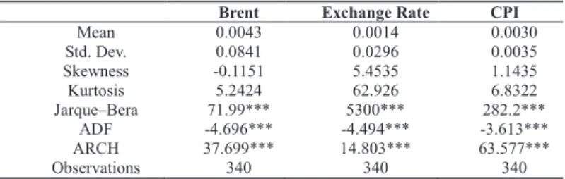
3. Data
Our estimations used the logarithmic differences of the seasonally adjusted monthly data for the period of August 1989 to December 2017. Crude oil price data were obtained from Thomson Reuters statistics, available via Independent Statistics and
Brent Exchange Rate CPI
Mean 0.0043 0.0014 0.0030
Std. Dev. 0.0841 0.0296 0.0035
Skewness -0.1151 5.4535 1.1435
Kurtosis 5.2424 62.926 6.8322
Jarque–Bera 71.99*** 5300*** 282.2***
ADF -4.696*** -4.494*** -3.613***
ARCH 37.699*** 14.803*** 63.577***
Observations 340 340 340
Note: The maximum number of lags for the ADF test selected by the Schwarz information criterion was 16. For CPI the base period is January 2010.
Table 1. Descriptive statistics for logarithm differences of the seasonally adjusted monthly data
Analysis of the US Energy Information Administration. The exchange rates and CPI are calculated using the data reported by the Bank of Korea and the national statistics of South Korea, available via the Korean Statistical Information Service.
The mean values of the logarithmic differences are positive (Table 1), showing an increasing trend in the variables. The standard deviation values show that the crude oil price and exchange rate are more volatile than the CPI. The skewness and kurtosis values show that the logarithmic differences are not distributed normally. The Jarque- Bera test confirms that the sample data have skewness and kurtosis not matching a normal distribution. The Lagrange multiplier test for an ARCH effect shows that the series exhibit conditional heteroskedasticity. This means the logarithmic differences fluctuate around a constant level, but exhibit volatility clustering. The augmented Dickey-Fuller (ADF) test for unit root returned values smaller than the critical values at the 1% significance level, thus strongly rejecting the presence of unit root.
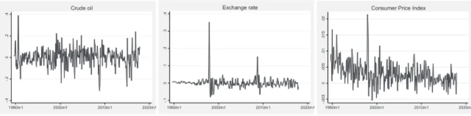
The Wald test for the presence of structural breaks led us to reject the null hypothesis of no structural break at the 1% significance level. The estimated break date was January 1998 for the exchange rate and March 1998 for CPI. The logarithmic differences are depicted in Figure 1.
4. Empirical findings
The estimations of the EGARCH model (Table 2) show a significant impact (at the 1% significance level) of previous month’s values and dummy variables for structural breaks. For crude oil, past negative information has a stronger effect on conditional
-.4-.20.2.4
1990m1 2000m1 2010m1 2020m1
Crude oil
-.10.1.2.3.4
1990m1 2000m1 2010m1 2020m1
Exchange rate
-.0050.005.01.015.02
1990m1 2000m1 2010m1 2020m1
Consumer Price Index
Figure 1. Logarithmic differences of the seasonally adjusted monthly data
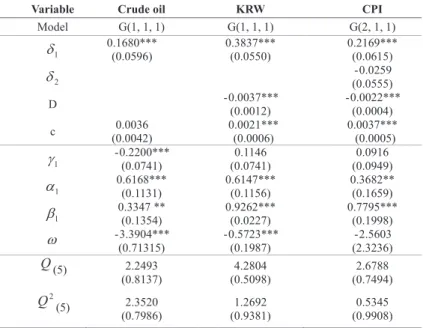
variance than past positive information. However, this asymmetric effect is smaller than the symmetric effect of past information. The symmetric effect of past information and the impact of past volatility on the variance of all three variables is positive and statistically significant at a 1% to 5% significance level. The portmanteau (Q) test statistic for white noise indicates that the standardised residuals and their squared values do not contain autocorrelation up to order 5.
Table 3 shows that crude oil price Granger-causes CPI in mean within two months (as the coefficient of the previous month is significant) and in variance within six months (as the coefficients of the previous five months become significant). That means the previous month’s price of crude oil helps predict the current month’s CPI.
The volatility of the crude oil price over the previous five months helps predict the volatility of CPI in the current month.
Exchange rate Granger-causes CPI in mean within two months (as the coefficient of
Variable Crude oil KRW CPI
Model G(1, 1, 1) G(1, 1, 1) G(2, 1, 1)
δ1 0.1680*** (0.0596) 0.3837*** (0.0550) 0.2169*** (0.0615)
δ2 (0.0555) -0.0259
D -0.0037***
(0.0012) -0.0022***
(0.0004)
c 0.0036
(0.0042) 0.0021***
(0.0006) 0.0037***
(0.0005)
γ1 -0.2200***
(0.0741) 0.1146
(0.0741) 0.0916
(0.0949)
α1 0.6168*** (0.1131) 0.6147*** (0.1156) 0.3682** (0.1659)
β1 0.3347 ** (0.1354) 0.9262*** (0.0227) 0.7795*** (0.1998)
ω -3.3904***
(0.71315) -0.5723***
(0.1987) -2.5603
(2.3236)
Q(5) 2.2493
(0.8137) 4.2804
(0.5098) 2.6788
(0.7494)
Q2(5) 2.3520
(0.7986) 1.2692
(0.9381) 0.5345
(0.9908) Note: The numbers in parentheses are standard errors.
Table 2. Results of the EGARCH model
the previous month is significant). That means the previous month’s exchange rate helps to predict the current month’s CPI. CPI Granger-causes exchange rate in variance within two months (as the coefficient of the previous month is significant). That means the volatility of CPI in the previous month helps predict the volatility of the exchange rate in the current month.
5. Concluding remarks
We estimated the impact of the crude oil price on exchange rate and CPI and the relationship between the exchange rate and CPI for the case of South Korea. Our estimations, which are based on seasonally adjusted monthly logarithmic differences, showed that the exchange rate and CPI Granger-cause each other. The crude oil price Granger-causes CPI but not the exchange rate. Nevertheless, considering the relationship between crude oil and other important economic variables, as described in the introduction, the crude oil price could affect the exchange rate via price level and other economic variables.
References
Bollerslev, T. 1986. “Generalised autoregressive conditional hetroscedasticity”. Journal of Econometrics 31: 307–327.
Cheung, Y. and L. K. Ng. 1996. “A causality-in-variance test and its application to
Period
Causality-in-mean Causality-in-variance Crude oil
KRW to
Crude oil CPI to
KRW to CPI
CPI to KRW
Crude oil KRW to
Crude oil CPI to
KRW to CPI
CPI to Previous month 0.3657 9.2589 10.6118 1.0085 -0.5311 -0.0055 -0.7071 78.7950 KRW Previous 2 months -0.1871 6.0471 7.0328 0.2454 -0.8734 -0.5025 -0.9672 55.2166 Previous 3 months -0.0117 4.5394 5.8523 -0.0305 -0.2966 -0.7478 -1.1923 44.6871 Previous 4 months -0.0257 3.6445 4.7272 -0.3433 -0.4830 -0.9293 -1.3100 38.6547 Previous 5 months -0.1686 3.3078 4.0912 -0.6096 -0.4471 3.7117 -1.4730 34.3369 Previous 6 months 1.1733 2.7402 4.1988 0.4000 -0.6782 3.1001 -1.5651 31.1417 Previous 7 months 0.8230 2.5797 3.9206 0.1397 -0.2544 2.6785 -1.6860 28.6958 Note: Generalised chi-square test statistics suggested by Hong (2001) are presented. Asymptotic critical values are 1.645 at the 5% level and 2.326 at the 1% level.
Table 3. Causality relationship
financial markets prices”. Journal of Econometrics 72(1): 33–48.
Engle, R. 1982. “Autoregressive conditional heteroscedasticity with estimates of the variance of United Kingdom inflation”. Econometrica 50(4): 987–1007.
Hong, Y. 2001. “A test for volatility spillover with application to exchange rates”.
Journal of Econometrics 103(1-2): 183–224.
Hsing, Y. 2016. “Is real depreciation contractionary? The case of South Korea”.
Economics Bulletin, AccessEcon 36(4): 1951–1958.
Kim, H. S. and J. Baek. 2013. “Assessing dynamics of crude oil import demand in Korea”. Economic Modelling, Elsevier 35(C): 260–263.
Kim, K. 2012. “Oil price shocks and the macroeconomic activity: Analyzing transmission channels using the new Keynesian structural model (in Korean)”.
Economic Analysis (Quarterly), Economic Research Institute, Bank of Korea 18(1): 1–29.
Masih, R., Peters, S. and L. De Mello. 2011. “Oil price volatility and stock price fluctuations in an emerging market: Evidence from South Korea”. Energy Economics, Elsevier 33(5): 975–986.
Nelson, B. D. 1991. “The conditional heteroskedasticity in asset returns: A new approach”. Econometrica 59(2): 347–70.
Shin, E. and S. Tim. 2011. “Joint stockpiling and emergency sharing of oil:
Arrangements for regional cooperation in East Asia”. Energy Policy, Elsevier 39(5): 2817–2823.
Thenmozhi M. and N. Srinivasan, 2016. “Co-movement of oil price, exchange rate and stock index of major oil importing countries: A wavelet coherence approach”.
Journal of Developing Areas, Tennessee State University, College of Business 50(5): 85–102.