Strategies for an Optimized simulation of granular particles in a Newtonian Fluid, Part 2: Numerical algorithms(Mathematical Aspects of Complex Fluids and Their Applications)

Strategies

for

an

Optimized simulation of granular

particles

in

a

Newtonian

Fluid,

Part 2:

Numerical

algorithms

Ivaylo Petrov Tabakov\ddagger\dagger_,

Institute of Mathematics and Informatics, Bulgaria

Hans-Georg Matuttis, Takafumi Suzuki\dagger,

\dagger_{University of Electro-Comm unications, Department of Mechanical Engineeringand}

Intelligent Systems, Chofu, Chofugaoka 1-5-1, Tokyo 482-8585, Japan

Abstract

Wedescribe

our

experienceswith sparse solvers for the stationary

incompress-ible Navier-Stokesequation on a Friedrichs Keller grid with various boundary

conditions. We simulate polygonal granular particles in a surrounding

in-compressible fluid in

a

$\mathrm{P}2\mathrm{P}1$ Galerkin finite element discretization, whereby

Newton-Raphson iteration turns out to be surprisingly robust. For the

inver-sionof the Jacobian, itturns out that from thevarious sparse algebraic solvers

in

use

in the numerical community, even GMRES does not reach the necessary

accuracy, and only BiCGSTAB(l) gives satisfying results.

4

Introduction

The simulation of the interaction between fluids and granular material involves many

preliminary stepswhich simplifiesordecrease thedegreeof freedornofthe initial problem.

The findingsin research introduced in the article are preliminary for the $\mathrm{i}\mathrm{m}\mathrm{p}\mathrm{l}\mathrm{e}\mathrm{m}\mathrm{e}\mathrm{I}\grave{[perp]}\mathrm{t}\mathrm{a}\mathrm{t}\mathrm{i}\mathrm{o}\mathrm{n}$

of a full simulation containing polygonal granular particles modeled with the discrete

element method and the fluid modeled with the Galerkin finite element discretization of

the incompressible Navier Stokes equation.

For an efficient implem entation, the use of unstructured grids is necessary, as well as

the solution of the nonlinear system of equations resulting from the discretization, with

sparsematrix algorithm$\mathrm{n}\mathrm{s}$. Inthiswork, we investigate which of the considerablevarietyof

Krylov-space iterative solvers gives satisfying results for structured grids and is therefore

a candidate for the use with unstructured grids.

We

are

dealing exclusively here with solutionofthestationaryNavier-Stokesequation.

though our final aim is an implementation of the time-dependent equations, because the

solution of the stationary problem is necessary to obtain consistent starting values for

the time-dependent Navier-Stokes equation in the DAE-form ulation (see the first part of

this article on the previous pages). From the structure of the problem , it is clear that

the non-stationary

case

is numerically more benign, because the mass-term dominates,

where the non-linearities and the stiffness-matrix arerescaled with thetime-stepandtheir

contribution is much smaller than in the stationary problem.

5

Discretization

and Band

structure

As the work-horse for this investigation, we choose the Flow5-code by John $\mathrm{B}\mathrm{u}\mathrm{r}\mathrm{k}_{\epsilon}\mathrm{a}\mathrm{r}\mathrm{d}\mathrm{t}[5])$

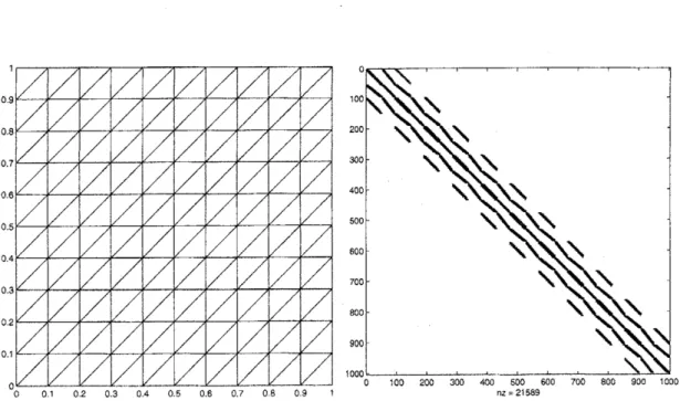
Figure 8: Thestructure of the Jacobian for the Friedrichs Keller grid (left, herefor cavity

flow) is a band matrix (right)

Navier-Stokes equation

$u \frac{\partial u}{\partial x}+v\frac{\partial u}{\partial y}+\frac{1}{\rho}\frac{\partial p}{\partial x}-\iota/\ovalbox{\tt\small REJECT}\frac{\partial^{2}u}{\partial x^{2}}+\frac{\partial^{2}u}{\partial y^{2}}\ovalbox{\tt\small REJECT}=0$, (S)

$u \frac{\partial v}{\partial x}\dashv- v\frac{\partial v}{\partial y}+\frac{1}{\rho}\frac{\partial p}{\partial y}-\iota/\ovalbox{\tt\small REJECT}_{\frac{\partial u}{\partial x}\frac{\partial vv2\ovalbox{\tt\small REJECT}}{\partial y}}^{\frac{\partial^{2}\mathrm{s})}{\partial x^{2}}+\frac{\partial^{2}}{+\partial y}}==00$

,

$(10)(9)$

for the $\mathrm{v}\mathrm{e}\mathrm{l}\mathrm{o}\mathrm{c}\mathrm{i}\mathrm{t}\mathrm{y}- \mathrm{f}\mathrm{i}\mathrm{e}\mathrm{l}\mathrm{d}\epsilon$; _$?\iota.v$ in $x$,$y$-direction and the pressure field with dynamic viscosity

$lJ$ in a Galerkin Finite Elem ent Method with $\mathrm{P}2\mathrm{P}1$ elements. The discretized problem

is a system of nonlinear equations with velocities $u_{i}$ and $v_{i}$ x- and $\mathrm{y}$-direction

on

all $\mathrm{i}$

integration points,

as

wellas on the pressures$\hat{p}_{k}$ on all integrationpoints $k$ (whichfor the

$\mathrm{P}2\mathrm{P}1$-elements is only

a

subset of the $\mathrm{i}$ mesh-pointsof the velocities),

so

that the vector

of all variables

$X=$ $(u_{12,\ldots i^{l}1}, uu\mathrm{L}’, v_{2}, \ldots v_{i},p_{1}j’ p_{2}, \ldots p_{k})$.

ThestationaryNavier-Stokes equations eqns. (8-10) consist formally

a

field problem$\mathcal{F}(u, v, p)=$

$0$, and the corresponding discretized problem

$\overline{F}(X)=0$,

is a conventional root-finding problem for non-linear equations. The iterative solution by

the Newton-Raphson method

$\vec{X}_{n+1}=\vec{X}_{n}-(\nabla\vec{F}(\vec{X}_{n}))^{-1}\vec{F}(X_{n})\neg$ (10)

proved to be stable enough during the whole of the investigations;

no

additional

$X_{0}$. The kernel of the iteration is the solution of the linear system

$\triangle\vec{X}=\check{x}(\nabla\vec{F}(\overline{X}_{n}))\ovalbox{\tt\small REJECT}_{A}\vec{F}(\vec{X})-1\mathrm{m}_{b}^{7b}$

’ (12)

where $A$is matrixofthe Jacobian and $\triangle x$ is the residual of the solution. We have started

the Newton-Raphson iteration with constant non-zero initial guesses, the initialization

with

zero

initial guessis bothunphysical and gave spurious convergence for

some

iterative

solvers. For most boundary conditions investigated, three iteration steps

were

enough,

afterthat the solution changed only marginally.

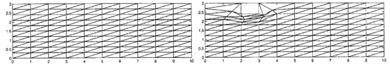
Figure 9: Friedrichs-Keller gridsused for the simulation ofpipe flow and pipe How below

a protruding step (inflowon the left, outflowontheright, i.e. open boundaries

on

the left

andright end with

a nonzero

velocity gradient and fixed boundaries

on

top andbottom).

The grid points around the step in the grid on the right were chosen to minimize the

dislocation oftheothergrid points, not to minimize theerror in thespacialdiscretization.

For afinite-element discretization with$\mathrm{I}^{)}2\mathrm{P}1$-elem ents,one element has approximately

$n=15$ degrees offreedom, 6pointsfor $u$, 6points for$v$and 3 points for$p$, though apoint

belongson averageto $m=3$ elements. The dimensions of$\nabla F$for a $\mathrm{F}\mathrm{r}\mathrm{i}\mathrm{e}\mathrm{d}\mathrm{r}\mathrm{i}\mathrm{c}\mathrm{h}\iota \mathrm{i}\sigma- \mathrm{K}\mathrm{e}\mathrm{l}\mathrm{l}\mathrm{e},\mathrm{r}$ grid

(the usual Finite-Element grid,

see

Fig. 8, left) with $b$ _{$=(2\cross l_{x}\mathrm{x} ly)$} elements has the

linear dimension$l=$ $(2\cross l_{x}\cross l_{y})\mathrm{x}$$n/m$. Because thereareonlyentries foradjacent degrees

offreedom, the matrix is sparse and banded with bandwidth $(l_{x}\mathrm{x} ly)$ (see Fig. 8, right).

Forthe reference runs, wehave used the $\mathrm{L}\mathrm{U}$-decomposition (for theformulation ofVF as

full matrix) and the incomplete $\mathrm{L}\mathrm{U}$-decomposition (threshold $10^{-10}$, for the formulation

of$\nabla\vec{F}$as sparse matrix). For general problems with $l$ variables, thenumber of operations

necessary for a solution with the $\mathrm{L}\mathrm{U}$-decornposition is of the order of $l^{3}$, which would

be prohibitive for a general matrix which occurs for unstructured grids. For the banded

matrix of the Friedrichs-Keller-Grid, the number ofoperations is one order ofmagnitude

less, only $lb^{2}$.

6

Eigenvalue

Analysis

For finite difference discretizations, the discretized solution of the flow-lines corresponds

directlyto the continuumsolution. and the properties can be compareddirectly For the

Gaierkin Finite Elementmethod, which introduces basis functions and additionaldegrees

of freedom via integration, such acomparison is

more

problematic. One possible strategy

is to analyze the problem[26] in terms of the eigenvalue spectrum of the Jacobian. The

solution of the linearsystem in eq. (12) with the Jacobian $\nabla\vec{F}(\vec{X}_{n})$. Because the choice

of Krylov-space solvers depends

on

the eigenvalue spectrum of the matrix of the linear

system, it is worthwile to investigate the eigenvalue spectrum of the Jacobian to develop

an insight about the convergence of the algorithms depending on the physical problem.

It turns out that the eigenvalues ofthe Jacobian depend crucially

on

the vorticity in the

problem and the eigenvalueschange with each Newton-Raphson iteration eq. (11). In the

following, we have performed the Newton-Raphson iteration with $\mathrm{L}\mathrm{U}$-based inversion of

the Jacobian with constant initial vector.

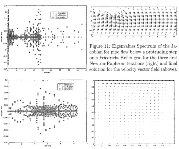
Forthe pipe flow (Fig.9 left), the eigenvalues forthe first Newton-Raphson iteration

are

along the cor plex axis, along the real axis, and

a

third group is spread out fan-like

symmetrically around the real axis (Fig. 10). With proceeding iterations, the eigenvalues

of the fan-like group are drawn towards the real axis. The Newton-Raphson iteration

eq. (12) converged basically within three steps to ten digits accuracy

.

as

can

be

seen

by

the fact that in the plot of thle eigenvalues, (Fig. 10, left), the symbols for the second

iteration $(’\backslash +’.)$

are

basically in the center of the symbols for the third iteration $(^{\rangle\backslash }’ 0")$.

Convergence within three steps was also observed for the geometries below. Forthe flow

below a step (Fig.9 right), the eigenvalue distribution is about thesame as for the pipe

flow, (Fig. 11, note the different scale of the real axis in comparison to Fig. 10.) Afterthle

third iteration, some butterfly-like clouds remain relatively far from the real axis. For

the pipe-flow below

a

step, the Jacobian has larger eigenvalues (Fig. 11, left) than the

Jacobian for unperturbed pipe-flow (Fig.10, left), whereas the streamlines for the flow

around the obstacle show smaller velocities at the boundary

near

the obstacle (Fig. 11,

right) than for the unperturbed flow (Fig.10 right). As the Jacobian enters the

Newton-Raphson iteration eq. 12 in the denominator,

so

that its large eigenvalues cause sm all

contributions, plausible to conclude that the small structures in the flow correspond to

large eigenvalues in the Jacobean, and viceversa.

In

case

ofcavity flow, at the first Newton-Raphson iteration the eigenvalues

are

near theaxis, andduring theiterationsspreadout into similar butterfly-like structures(Fig. 12, left) as inthe

case

of the flow below astep (Fig. 11). As the similaritybetween the

cavity-fiow and the flow below the step, one

can

conclude that the butterfly-like structures in

the eigenvalue spectrum

are

associated with the vorticity in the system.

Figure 12: Eigenvalues Spectrum of the Jacobian Matrix for cavity flow using Friedrichs

Keller grid and the final solution for the velocity vector field. The upper boundary has

a

constant flow in $\mathrm{x}$-direction and zero velocity in $\mathrm{y}$-directionimposed, at all other walls

fixed boundary conditions are set. The right boundary is at $x=1.\mathrm{O}$, only the vector for

thle velocity of the upper right boundary point extends beyond.

stacles), the eigenvalue spectrum is “almost purely reai”. The eigenvalue analysis of the

Jacobean initialized with the correct final solution (Hagen-Poiseulle flow) might give the

$\mathrm{i}$mpression that purely real solvers are suitable for the problem. In case of cavity flow,

with the approachto thestationary numeric solution the eigenvalues runs away fromthe

real axis, and the necessity for solvers for problems with complex eigenvalue spectrum

becomes clear. Because the im aginarypart of the eigenvalues

can

become arbitrary large

in the presence ofvortices, linear solvers are needed which are explicitly constructed for

problems where the corresponding matrix

can

contain complex eigenvalues.

6.1

Choice

of

solvers

There

are

twoclasses of iterative solvers whichcanbe used onunstructuredgrids:

Station-$\mathrm{a}\mathrm{r}\mathrm{y}/\mathrm{R}\mathrm{e}\mathrm{l}\mathrm{a}\mathrm{x}\mathrm{a}\mathrm{t}\mathrm{i}\mathrm{o}\mathrm{n}$ methods, which are basically improved versions of the Jacobi-Iteration,

Conjugate Gradient method. The drawback of the original relaxation methods (Jacobi,

Gauss-Seidel, Successive Overrelaxation) was the slow convergence due to the small

cur-$\mathrm{v}\mathrm{a}\mathrm{t}\mathrm{u}\mathrm{r}\mathrm{e}/$ largelength-scale introduced bythe “smoothing” inherent in the relaxation. This

problem can be

overcome

in the Multigrid methods, which solve the equations

simuita-neously also on

coarser

grids, so that the information is transferred between the length

scales. The appealing feature oftransferring length scales ofthe solutiondirectly in

geo-metrical terms becomes lost when unstructured meshesareused, where so-calledalgebraic

multi grid method have to be

use

to compensate for the loss of geometrical information

in the corresponding matrix. The manuals of such algebraic multi grid packages (e.g.

$\mathrm{U}\mathrm{G}[2])$ are usually already much thicker than

some

books

on

linear algebra, and learning

thehandling

even

as black boxes takes considerable time. As

we

want to put our effortin

the solution of the Navier-Stokesequations, not in the underlying algebraic methods, we

choose instead Krylov-space solvers for sparse matrix methods, which are based more on

algebraic than

on

geometric considerations. Apart from the fact that the replacement of

the$\mathrm{L}\mathrm{U}$-decomposition in the original code is straightforward, afurther advantage isthat

there

are

criteria irr terms of eigenvalues, although there is no guarantee of convergence

(in the

case

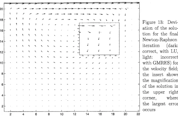
of Relaxation method, thereisn’t, either.)

Figure 13:

Devi-than of the

solu-tion for the final

Newton-Raphson

iteration (dark:

correct, with $\mathrm{L}\mathrm{U}$,

light: incorrect

withGMR ES) for

the velocity field; the insert shows

the magnification

of the solution in

the upper right

corner, where

thle largest error

occurs

6.2

Nonstationary Iterative

Methods(Krylov

Space

Methods)

The ancestor of Krylov-Space methods (see Ref. [1] for

an

overview), which try to solve

a linear system $Ax=b$ by minimizing the residuum vector $r=Ax-b$, is the Conjugate

Gradient method (GC), which works only for positive definite $A$. Newer methods have

been developed for more general

cases.

We did not

use

preconditioners, because for

isunclear whata good” preconditioner might be. All standard methods like Bi-conjugate

Gradient, Conjugate Gradient Squared and Bi-conjugate Gradient Stabilized failed for the solution, both in the MATLAB-implementation

as

well

as

in the Implementation of

Ref. [1]. Only with GMRES and BiCGSTAB(l)[lS], solutions for the Newton-Iteration

could be obtained at all

6.3

GMRES

-

a surprising

failure

The Generalized Minimal Residual Method (GMRES) is widely used in fluid mechanics

in the so-calledNewton-GM RES-method for the Navier-Stokes equation forcompressible

flows. For our incompressible problem, it

never

converged to theexact(LU) solution with

more than three digits accuracy. This would not so bad for the velocity in Fig. 13, but it

is unacceptable for the pressure in Fig. 14, as the violation of the continuum equation in

a DAE-formulation will lead to a degeneration of the solution away from the constraint

manifold. Wetriedout different initialsolutions, but this did notimprovethe convergence

in any way. The badconvergence oftheNewton-Raphson iteration with GMRES is

even

more surprising asthe Newton-Raphson iterationis asecond ordermethod, i.e. itdoubles

the accuracy of the solution in each iteration. This has the downright magic effect that

with a preliminary solution $x_{n}$ and a Jacobian or its approximant which are correct to

$\mathrm{k}$ digits in the n-th step, the next solution

$x_{n+1}$ will exhibit $2k$correct number of digits.

Not

even

this formidableproperty

seems

to further the accuracy of the solutions obtained

with GMRES so we have to conclude that forour incompressibility problem, GMRES is

inherently inapplicable.

Figure 14: Comparison between pressure vectors obtained via GMRES and LU

respec-tively, for the 3rd iteration of the system in Fig. 8; the GM RES-pressure deviates from

the “numerically exact” $\mathrm{L}\mathrm{U}$pressure constantly

over

the whole grid.

6.4

BiCGSTAB(1)-

the

successful

solver

BiCGSTAB(l) - Bi-Conjugate Gradient Stabilized(l)[18], is

newer

than other methods,

so it has not yet found its way in standard references like Ref. [1]. It

was

explicitly

built for problems with complex eigenvalues spectra to

overcome

the problems inherent in

BiCGSTAB

and GMRES and it

was

the only iterative linear solver which converged

within the desired tolerance. In contrast to other Krylov-Space methods. BiCGSTAB(l)

does not only

use

the residual $r.–Ax$ $-b$, but also the ”shadow residual” $r\sim=\tilde{x}^{T}A-\tilde{b}^{T}$.

Using

a

zero-vector for the initialization lead to spurious

convergence,

so

instead we

choose aconstant

non-zero

vector. We

use

BiCGSTAB(4) as well as BiCGSTAB(8) and,

apart from manually adjustment of the tolerance and the maximum number ofiterations,

there

were

no problem $\mathrm{s}$withthe convergence. BiCGSTAB(l)

seems

to thebest choice for

the time-dependent solution of the Navier-Stoke Equation for incom pressible flow with

vortices orfurther

more

solver for the granular-particle - fluid system sil ulation.

Figure 15: Convergence diagram ofBiCGSTAB(4) for the system in Fig, 8

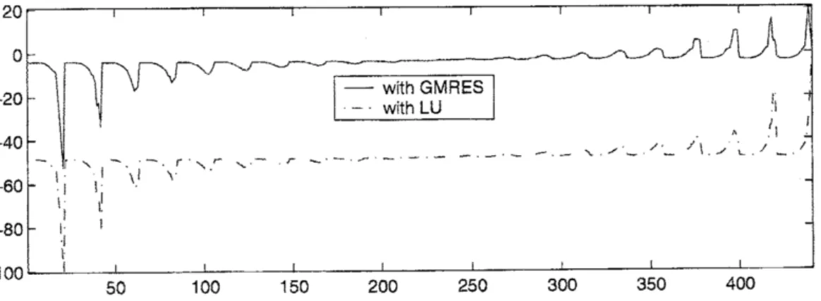
Fig. 15 shows the convergence of the

no

rm of the residual $|r|=|b-Ax^{(\mathrm{i})}|$ with

BiCGSTAB(4) to a given accuracy of $10^{-\mathrm{S}}$

.

The solver converges to tolerance

approxi-mately 10 after about 8000 BiCGSTAB(l)-iterations . For each Newton-Raphson

iter-ation, e.g. three, these 8000 BiCGSTAB(l)-iterations must be repeated, so that a total

of 24.000 BiCGSTAB(l)-iterations is necessary. This looks like a relatively costly

perfor-mance, but for a simulation of the time-dependent Navier Stokes equation, only for the

initial timestep the solution has to becomputed from scratch, using this many iterations

in the linearsolver; for the subsequent time-steps, the previous flow patterns

can

be used

as an initial guess which reduces the number of BiCGSTAB(l)-iterations, and usually,

only a single Newton-Raphson iteration is necessary.

7

Summary

and

Conclusions

We have investigated the solution of the stationary Navier-Stokes equations for the

in-com

npressible case with Newton-Raphson solution of the equations resulting

Galerkin-Finite element discretization for various geometries and have compared the perform ance

of different linear solvers for the inversion of the Jacobian in the Newton-Raphson

pro-cedure. Convergence was reached within three to five iterations. Except GMRES and

BiCGSTAB(l), all other solvers among the large variety of Krylov-Space solvers failed to

converge

or

crashed already intheinitial problem. Though GMRESisapopular solverfor

thecompressible Navier-Stokesequations, asdocumented by the existence of the

cient for all problems we investigated. Only BiCGSTAB(l), with $l\geq 4$ gave satisfying

solutions for all test cases in comparison with the ”numerical exact” solution for

LU-decomposition. The next step in the investigation will be the solution of time-dependent

problem for the

same

boundaryconditions, using thestationarysolutions obtainedin this

work

as

initial guess.

References

[1] R. Barrett, _{M. Berry, T. F Chan,J.}

Dem-mel, J. Donato. J. Dongarra, V. Eijkhout,

R.Pozo, C.Romine,andH. Van derVorst.

Templates

_for

the Solution

_of

Linear

Sys-tems: Building Blocks

_for

Iterative

Meth-ods, 2nd Edition. SIAM, _{Philadelphia,} $\mathrm{P}\mathrm{A}_{\mathrm{t}}$ 1994.

[2| P. Bastian, K. Birken, K. Johannsen,

S. Lang, N. Neuss, H. Rentz-Reichert, and

C. Wieners. Ug- a flexible software

tool-box for solving partial differential

equa-tions. Computing and Visualization in

Science Volume 1, $pp$. 27-40, 1997.

[$3_{\rfloor}^{\rceil}$ J. Bey. Tetrahedral gridrefinem $\mathrm{e}\mathrm{n}\mathrm{t}$.

Corn-puting Volume 55, pP. 355-378, 1995.

[4] J. Bey. A$GM\mathit{3}D$ Manual, Repor$rtNr$. 50,

$SFB\mathit{3}\mathit{8}\mathit{2}$. Math. II st Univ.Tiibingen,

1996.

[$5|$ John Burkardt. http:$//\mathrm{w}\mathrm{w}\mathrm{w}$

.

csit

.

$\mathrm{f}\mathrm{s}\mathrm{u}$. $\mathrm{e}\mathrm{d}\mathrm{u}/\sim$burkardt/.

[$6|$ Sydney Chapman and T. $\mathrm{G}$ Cowling.

The Mathernatical Theory

_{of Non-uniform}

Gases, _{Cambridge Unersity} Press, _Cam

-btidge, 1970.

[7] P. A. Cundall and 0. D. L. Strack. A

dis-crete numerical model for granular

assem-blies. Geotechnique, 29(1):47-65, 1970.

[8] E.Hairer and G.Wanner. Solving

Or-dinar.y

_Differential

Equations $II$,

Stiff

and Differential-Algebraic Problems,

vol-ume II of Springer Series in Computa-tionalMathematics. Springer. Berlin,

Hei-delberg, New York, 2 edition, 1996.

[9] U Frisch, _B. Hasslacher, _{and Y. Pom eau.}

Lattice-gasautomata for the navier-stokes

equation. Phys. Rev. Lett. Volume 56, $pp$.

1505-1508, 1986.

[10] $\mathrm{R}.\mathrm{A}$

. Gingold and $\mathrm{J}.\mathrm{J}$

.

Monaghan.

Smoothed particle hydrodynamics:

the-oryandapplicationto non-spherical stars.

Mon Nat. R. Astron Soc, 181375-389,

1977.

[11] E. Hairer, S. P. Norsett, _{and G.}

Wan-ner. Solving Ordinary

_Differential

Equa-tions $I$,

Nonstiff

Problems, volume I of

Springer Series in Computational

Mathe-matics. Springer, Berlin, Heidelberg, New

York, 2.nd edition, 1993.

[$12_{\rfloor}^{\rceil}$ F.H. Harlow and $\mathrm{J}.\mathrm{E}$

.

Welch. Numerical

calculation of time-dependent viscous

in-com pressibleflow, _{Phys. Fluids Volume 8,}

pp. 2182-2189 1965

[$13_{\rfloor}^{\rceil}$ Kai Hdfler, Matthias M\"uller. Stefan Schwarzer, and Bernd$\mathrm{n}\mathrm{d}$ Wachm ann.

Inter-acting particle-liquid systems. High

Per-formance

Computing inScience and

Engi-neering E. Krause W. Jdger$eds$.Springer,

1998.

[14] Takeo Kajishima. Num ericalinvestigation

of multiscale interaction between

turbu-lent flow and solid particles. In The

₅₄

th

Nat. Cong

_of

Theoretical

es

Applied

Me-chanics, Tokyo, Japan, 2005.

$\downarrow\dagger 15]$ S. KoshizukaandY. Oka. Moving-particle

semi-implicit method forfragmentationof

incompressible fluid lust. Sci. $Eng$

.

Vol-$ume\mathit{1}\mathit{2}\mathit{3}_{y}pp$. 421-434, 1996.

[16] S. Koshizuka, H. Tarnako, and Y. Oka. A

particlemethod forincompressibleviscous

flow with fluid fragmentation. Comput.

Fluid Dynamics J. Volume 4, $pp$.

29-4

$\theta$,

$|’ 17|$ A. J. C. Ladd and R. Verberg.

Lattice-boltzmann sixnulatiolls of particle fiuid

suspensions. J. Stat. Phys. Volume 104,

pp. 1191 - 1251, 2001.

$\llcorner\ulcorner 1\mathit{8}]$ Gerard

$\mathrm{L}$ G.Sleijpen and Diederik

R.Fokkema Bicgstab(1) for linear

equa-tions involving unsymmetric matrices

with complex spectrum Electron. Trans.

$N\uparrow lm\mathrm{r}7$. Anal. Volume 1. _$pp$ 11-32, 1993

[$19|\mathrm{B}$ $\mathrm{D}$ Lubachevsky and F. H. Stillinger

Geometric properties of random$\mathrm{n}$disk pack-$\mathrm{i}_{\mathrm{I}1}\mathrm{g}\mathrm{s}$

.

J. Stat. Phys. $60(^{r}|\lrcorner/6):561- 583$,

1990.

[$20_{\rfloor}^{\rceil}$ S. Luding, $\mathrm{E}$ Clement, A. Blumen, J.

Ra-jchenbach, and $\mathrm{J}$ Duran. Studies of

columns of beads under external

vibta-tions. $P/?7S$ Rev. $E$, 49(2):\perp 634, 1994.

$\lfloor|.21|$ H.-G. Matuttis, $\grave{[perp]}o\mathrm{b}\forall \mathrm{u}\mathrm{y}\mathrm{a}\mathrm{s}\mathrm{u}$ Ito, and

Alexander Schinner. Effect ot particle

shape on bulk-stress-strain relations of

granular materials. In Proceedin$\iota gs$

of

$Rlf\mathfrak{t}^{\prime Ig}$ Symposium on Mathematical $A_{\mathrm{b}-}$

pects

_of

Complex Fluids $III$, voiurne 1305

of RIM $S$ Kokyoroku series, pages 89-99,

Kyoto, 2003 RIMS.

[$22^{1}\mathrm{j}$ J. J. Monaghan. Smoothed particle$1_{1_{\iota}}\mathrm{v}\mathrm{d}\mathrm{r}\mathrm{o}-$

dvnaznics Annual Review

_of

Astronomy

and $A_{6}trophys\mathrm{i}c^{\backslash }s$, 30543-574, 1992

[$23_{\mathrm{J}}^{1}|$ J. ’1. Moveau Unilateral contact and dry

friction

in_finite

_freedom

dynamics, pages

1 82. Number 302. $\rfloor 988$

[21] J. J. Moreau. An expression of $\mathrm{c}\mathrm{l}\mathrm{a}\mathrm{s}\mathrm{b}\mathrm{i}\mathrm{c}\dot{\mathrm{c}}11$

dynamics, _{Ann.Inst. H.Poincare’Anal aVon}

$L\mathrm{i}n$’eaire, XXX(6):1-48, 1989.

[25] Shiro Okeda. Experiments on the

sound-velocity of granular beads (in Japanese).

Master’sthesis.The University of

Elcctro-Com munications. 2006.

[26] P.$\mathrm{A}\backslash \mathrm{I}$.Greshoand R.$\mathrm{I}_{\lrcorner}$.Sani. Incompressible

Flow and the Finite Element Method ,

Vol-$ume\mathit{1}$:

Advection-Diffusion.

John Wiley

and SonsXTD, NewYork, $\mathrm{N}\mathrm{Y}$, $2\mathrm{t}$)Ot). $\int.27|$ P.M.Gresho and$\mathrm{R}.\mathrm{L}$.Sani. Incompressible

Flowand theFiniteElementMethod

.

Vol-$l\mathit{7}r\iota e$ $\mathit{2}$:Isoth$errr\iota al$ Laminar Flow. John

Wiley and SonsXTD, New York, $\mathrm{N}\mathrm{Y}_{1}$

2000

[28] $\mathrm{W}$ E.Schiesser. The NumericalMethod

of

Lines: Integration

_of

Partial

_Differential

Equations. Academic Press, San Diego,

1991

[$29|\mathrm{S}$ Schwarzer, K. H\"ofler. C. Manwart,

B. Wachmarm, and H. Herrm anll.

Non-browniansuspensions: Simulationand

lin-ear response physica a 1999. In Proc..

Conf

on Percolation and Disordered $6’ys-$

tems. $\mathrm{R}\mathrm{a}1\iota \mathrm{s}\mathrm{c}1_{1}:_{1\mathrm{O}}1\mathrm{z}11\mathrm{a}\mathrm{u}\mathrm{s}\mathrm{e}\mathrm{I}1$_, Germany, July

1998

$\lceil 30_{\mathrm{J}}^{1}|$ Bernd $\mathrm{l}\mathrm{V}\mathrm{a}\mathrm{c}‘ 1\mathrm{l}\mathrm{n}\mathrm{t}\mathrm{a}\mathrm{n}\mathrm{n}$and Stefan Schwarzer.

Three-di mensional rnassively parallel

com-putingofsuspensions. Int J. Mod Phys. $C$

Volume $\mathit{9}(^{r}v)pp$ 759-775. 1998

[31] Toru Watanabe,_{Hiroshi Watanabe.}

Torni-ichi Hasegawa, and Takatsune Narumi

Flow analysis ofcomplex fluids through a

sm all orifice. In The

₅₄

th Nat. Cong

_of

$Theor\epsilon t\mathrm{i}cal$ $\mathrm{f}.\mathit{4}$ Applied Mechanics, Tokyo,

Japan, 2005.

[32] John $\mathrm{W}$Perram, John Rassm ussen, Eigil

Praestgaard, and Joel L.Lebowitz.

Ellip-soid contact potential: Theory and

reia-tion to overlap potentials. Phys. Rev. $E$_,