DOI http://dx.doi.org/10.5670/oceanog.2014.87 COPYRIGHT This article has been published in Oceanography, Volume 27, Number 4, a quarterly journal of The Oceanography Society

(1)

CITATION

Zwolinski, J.P., D.A. Demer, G.R. Cutter Jr., K. Stierhoff, and B.J. Macewicz.

2014. Building on fisheries acoustics for marine ecosystem surveys.

Oceanography 27(4):68–79, http://dx.doi.org/10.5670/oceanog.2014.87.

DOI

http://dx.doi.org/10.5670/oceanog.2014.87

COPYRIGHT

USAGE

Permission is granted to copy this article for use in teaching and research.

Republication, systematic reproduction, or collective redistribution of any portion of this article by photocopy machine, reposting, or other means is permitted only with the approval of The Oceanography Society. Send all correspondence to: [email protected] or The Oceanography Society, PO Box 1931, Rockville, MD 20849-1931, USA.

OceanographyTHE OFFICIAL MAGAZINE OF THE OCEANOGRAPHY SOCIETY

DOWNLOADED FROM HTTP://WWW.TOS.ORG/OCEANOGRAPHY

(2)

SPECIAL ISSUE ON FISHERIES OCEANOGRAPHY

Building^onFisheries Acoustics

for Marine Ecosystem Surveys

By Juan P. Zwolinski, David A. Demer, George R. Cutter Jr., Kevin Stierhoff, and Beverly J. Macewicz

NOAA Ship Bell M. Shimada is helping scientists gain valuable insight into the California Current Large Marine Ecosystem, a globally significant natural resource that stretches from Baja California to British Columbia. Photo Credit: NOAA OMAO

(3)

abundances to fluctuate naturally. Ideally, this information is obtained empirically from frequent fisheries-independent surveys (Gunderson, 1993).

The California Current Ecosystem and Its Forage Fish Community The California Current Ecosystem (CCE) spans the west coasts of Vancouver Island, Canada, the United States, and part of Baja California, Mexico (Longhurst, 1998). The CCE is a large upwelling marine ecosystem (Sherman and Duda, 1999), located in a transition zone between subtropical and sub-Arctic water masses, and exhibits highly variable productivity and diversity (Garibaldi and Limongelli, 2002). As in other upwelling ecosystems, the abundances of coastal pelagic fish species (CPS) in the CCE wax and wane cyclically (Baumgartner et al., 1992; Finney et al., 2002), alternately dominating the forage-fish assemblage (Alheit and Bakun, 2010). These oscilla- tions are due to periodic changes in the environment (MacCall, 2009; Zwolinski and Demer, 2014) but may be accelerated

or delayed by fishing pressure (Radovich, 1982; Zwolinski and Demer, 2012).

Probably the most well-known CCE fishery is the large sardine fishery that existed from Mexico to Canada during the first half of the twentieth century (Radovich, 1982). During the 1936–

1937 season, this fishery landed roughly 720,000 metric tons (mt) of sardine, comprising about one-third to one-half of the stock biomass (Wolf, 1992). This extreme harvest, coupled with environmental conditions unfavorable to sardine recruitment (Radovich, 1982; Jacobson and MacCall, 1995; Zwolinski and Demer, 2012), caused the catches to drop to less than half in 10 years, and to less than 10% of the maximum values before a moratorium was enacted in 1974 (Wolf, 1992). Without abundant sardine, the industrial infrastructure proved exces- sive for harvesting other CPS, and much of it was abandoned. During the 1960s to 1980s, the CPS fishery targeted northern anchovy (Engraulis mordax, here- after anchovy), with some opportunistic fishing on Pacific and jack mackerels (Scomber japonicus and Trachurus sym- metricus, respectively) and market squid (Doryteuthis opalescens). In the 1990s, the moratorium was lifted and the fishery switched its focus back to the then resurg- ing sardine stock. The sardine stock and harvest peaked circa 2006, and by 2013, both had receded to their lowest values in more than 20 years (Hill et al., 2014).

Coincident with the decline of the sardine stock, jack and Pacific mackerel were increasingly abundant within the survey region (Zwolinski and Demer, 2012).

Currently, sardine landings are small and declining, particularly in the northern CCE, and opportunistic fishing on mackerels and anchovy have been variable. In the northern CCE, hake and herring dominate the landings of forage fish.

In addition to the various fisheries, the INTRODUCTION

By an act of the US Congress, and multiple succeeding amendments and re- authorizations¹, US marine fisheries are moving away from single species management and toward an ecosystem approach (FAO, 2003). Consequently, efforts are underway to collect the vast amount of new information necessary for compliance. Fundamental to managing any fishery is knowledge of stock abundances, distributions, and age struc- tures, as well as life-history parameters such as recruitment success, and growth and natural mortality rates. Estimates of these parameters, presently obtained from a variety of sources and combined with commercial catch data in statistical stock assessment models, are used to estimate the abundance and trajectory of a population (Hilborn and Walters, 1992). To also manage the functioning of an ecosystem, fundamental information is needed about the numerous species comprising the food web, as well as information about their biotic and abiotic environments that may cause their

ABSTRACT. The National Oceanic and Atmospheric Administration Marine Fisheries Service endeavors to manage fish stocks with an ecosystem perspective. This objective requires an understanding of the effects of the environment and fishing on all major ecosystem components. For example, in large upwelling systems like the California Current Ecosystem (CCE), natural cycles in the oceanographic and atmospheric conditions appear to drive large fluctuations in the distributions and relative abundances of coastal pelagic fish species (CPS), for example, sardine, anchovy, mackerels, and herring. These changes may be accelerated or delayed by changes in mortality due to fishing or predation of larger fish, marine mammals, and seabirds. We suggest that the data necessary to manage CPS with an ecosystem perspective may be obtained from frequent surveys of multiple CPS and their biotic and abiotic environment. We show that this is practical with surveys based on a combination of acoustic and trawl sampling coupled with complementary measures from numerous other sensors. Such acoustic- trawl-method (ATM) surveys of the CCE were conducted during the spring and summer of 2012 and 2013. We present the results of these surveys, including the seasonal distributions and abundances of multiples of the most ecological and economically important CPS. These data hint at the ultimate potential of periodic surveys using ATM sampling augmented with physical oceanographic, zooplankton, ichthyoplankton, fish, seabird, and mammal investigations to characterize the ecosystems.

1 Magnuson-Stevens Fishery Conservation and Management Reauthorization Act of 2006, Pub. L. No. 109–479, 120 Stat. 3575 (2007)

(4)

CPS assemblage is essential prey for multiple species of tuna, shark, and salmon, as well as marine mammals and birds.

Because the roles of CPS in the CCE are manifold, their values to society and the ecosystem have been estimated to be many times more than those of just their commercial fisheries (Pikitch et al., 2014).

Therefore, to ensure food security and stewardship of the CCE and other ecosystems (FAO, 2012), the present methods of surveying, assessing, and managing marine fishes must be urgently improved, beginning with frequent surveys of multiple species and their environment.

Acoustic-Trawl Method Surveys The acoustic-trawl method (ATM) is a standard survey tool for estimating the abundances and distributions of krill (Hewitt and Demer, 2000); CPS such as sardine, anchovy, mackerels, and herring (Mais, 1974; Johannesson and Mitson, 1983); and semi-demersal species such as hake (Swartzman, 1997) and pollock (Williams et al., 2013). Its utility has been expanding to provide a broader ecosystem perspective (Demer et al., 2009b).

In the ATM, multifrequency split-beam echosounders (Figure 1) transmit sound pulses down beneath the ship and receive echoes from animals and the seabed in the path of the sound waves (Simmonds and MacLennan, 2005). The intensities of the echoes that are scattered

back (the backscatter signal) normal- ized to the range-dependent observational volume (the volume backscatter coefficient) provide indications of the target type and behavior. Fish, particularly those with highly reflective swimbladders (Foote, 1980), create high intensity echoes. Plankton, such as krill and salps, have acoustic properties closer to those of the surrounding seawater, and generally produce much lower intensity echoes. Nevertheless, they too can produce measurable backscatter, particularly when aggregated in large densities (Hewitt and Demer, 1991). Under cer- tain conditions, the summed intensities of the echoes from an ensemble of targets is linearly related to the density of the fish or plankton aggregations that contributed to the echoes (Foote, 1983).

This attribute of the summed intensities allows animal densities to be estimated by dividing the resulting “integrated backscatter coefficients” of the ensemble by the average echo energy from a repre- sentative animal. An estimate of animal abundance is then obtained by multi- plying the average estimated fish density and the survey area.

Target Identification and Density Estimation

Two of the principal challenges of acoustic sampling are to accurately apportion the backscatter to the various species that

contributed to the echoes and to estimate the mean backscatter for a repre- sentative individual from each species.

Backscatter from marine organisms is a function of body composition, shape, and size relative to the sensing-sound wavelength and orientation relative to the incident sound waves (Morse and Ingard, 1968). Scientific echosounders typically operate at multiple discrete frequencies or continuous-frequency bands between 18 kHz and 200 kHz, and may sample echoes from aggregations of organisms with individual lengths rang- ing from a few millimeters (e.g., large copepods and krill) to several centime- ters (e.g., sardine and mackerels). The frequency-dependent backscatter (backscattering spectra) is used to separate echoes from small and weak (e.g., zooplankton) and large and strong scatterers (e.g., fish with swimbladders), even when the former are aggregated in large densities or the latter are grouped in low num- bers. This information enables simul- taneous high-resolution sampling of multiple key components of marine ecosystems (Korneliussen and Ona, 2002) and systematic apportioning of their echoes. After the backscatter has been apportioned to the dominant taxonomic groups, further classification is generally performed using information from trawl (Figure 1) or plankton net samples (Karp and Walters, 1994; Simmonds

and MacLennan, 2005), or optical sampling (Demer, 2012).

Decades after a successful ATM campaign to survey abundant anchovy and mackerels off the coast of California (Mais, 1974), the ATM was reintroduced in the CCE in spring 2006 to sample the then abundant sardine population (Cutter and Demer, 2008).

Since then, this survey effort has continued and expanded through annual or semi-annual surveys (Demer et al., 2012; Zwolinski et al., 2012). Beginning in 2011 (Hill et al., 2011), the ATM estimates of sardine abundance and

FIGURE 1. (top) A conceptual image of acoustic-sampling beams pro- jecting from the National Oceanic and Atmospheric Administration’s newest Fisheries Survey Vessel Reuben Lasker, equipped with multi frequency split-beam (Simrad EK60; green) and multibeam (Simrad ME70; orange) echosounders, multibeam imaging sonar (Simrad MS70;

purple), and long-range omnidirec- tional sonar (Simrad SX90; gray).

(bottom left) A five-frequency echogram of a large fish school that was also sampled with a trawl. (bottom right) Sorting a trawl catch for identification of species and estimations of maturity, length, and age.

(5)

age structure have been incorporated in the annual sardine assessments. By 2011, the ATM results detected the onset of a recent period of low sardine productivity (Zwolinski and Demer, 2012). Here, we present the results of ATM surveys conducted in the CCE during both spring and summer in 2012 and 2013. The data are used to describe the abundances, distributions, and seasonal dynamics of multiple species of epipelagic fish in the CCE. Finally, we discuss the potential of the ATM surveys to provide the foundation for efficient sampling of species in multiple trophic levels to support fisheries management within an ecosystem perspective.

METHODS Survey Design

During the springs and summers of 2012 and 2013, part or all of the west coast of the United States was surveyed using the National Oceanic and Atmospheric Administration’s (NOAA’s) Fisheries Survey Vessel Bell M. Shimada and char- tered Research Vessel Ocean Starr (for- merly NOAA Research Vessel David Starr Jordan). Survey transects were reg- ularly spaced and nearly perpendicular to the coast, typically with separations of 10, 20, or 40 nautical miles. The spring surveys, typically 30 days in April, targeted the peak of the sardine spawning season when the sardine eggs provide further confirmation of the spatial extent and abundance of the stock (Lo et al., 2009).

The survey design was adjusted for the annual variation of the potential habitat of the northern stock of sardine (Figure 2;

Zwolinski et al., 2011). The summer surveys, typically lasting fewer than 80 days, spanned July and August. The

sampling encompassed the majority of the continental shelf northward of Point Conception, California, up to and beyond Vancouver Island, Canada (Figure 2).

This region included the potential sardine habitat and the historic distribution of hake (Agostini et al., 2006).

The spring surveys have been directed to sardine when the stock is more aggregated and deeper in the water column while spawning offshore of central and southern California, (Demer et al., 2012;

Zwolinski et al., 2012). The summer surveys have the advantages of longer daytime periods, calmer weather, coastal aggregations, and coincidence with the majority of the respective commercial fishing efforts. Surveys conducted during both spring and summer of the same year provide two independent estimates of the sardine stock abundance, with prime rel- evance for the annual assessments (Hill et al., 2014). Not shown here, the data from the summer 2012 and 2013 surveys were also used to assess semi-demersal hake (JTC, 2014).

Data Acquisition Acoustic Sampling

On both vessels, the acoustic systems operate at four discrete, narrowband frequencies centered at 38, 70, 120, and 200 kHz. Shimada also has an 18 kHz system. The echosounders were calibrated prior to each survey by the standard sphere method (Foote et al., 1987) using a 38.1 mm diameter, tungsten- carbide, 6% cobalt spherical target. During the survey, acoustic pulses were transmitted at least every 1.6 seconds while the vessels transited preselected transects at a constant speed of 10 knots. Because most CPS form schools in the upper mixed

layer during the day and disperse and rise to the surface during the night (Mais, 1974), the acoustic analysis was restricted to samples collected to 70 m depth during daylight hours, roughly between sunrise and sunset.

Trawling

Trawl sampling was conducted at night by returning to the positions where CPS schools where observed earlier that day.

The species composition in these regions was estimated from up to three trawl samples separated by roughly 10 nautical miles, comprising a “trawl cluster.”

During the day, sardine and mackerels form schools in the upper mixed layer, which extends as deep as 70 m in the

Juan P. Zwolinski ([email protected]) is Research Fisheries Biologist, Institute of Marine Sciences, University of California, Santa Cruz (Southwest Fisheries Science Center [SWFSC] affiliate), Santa Cruz, CA, USA. David A. Demer is Leader, George R. Cutter Jr. is Research Oceanographer, Kevin Stierhoff is Research Fisheries Biologist, all in the Advanced Survey Technologies Program, and Beverly J. Macewicz is Research Fisheries Biologist in the CPS Life-History Program, Fisheries Resources Division, SWFSC, National Marine Fisheries Service, National Oceanic and Atmospheric Administration, La Jolla, CA, USA.

FIGURE 2. Conceptual map showing the aver- age spring and summer distributions of Pacific sardine habitat along the west coasts of Mexico, the United States, and Canada. The dashed and dotted lines represent, respectively, the approximate summer and the spring position of the 0.2 mg m^–3 isoline of chlorophyll-a concentration. This isoline appears to oscillate in syn- chrony with the transition zone chlorophyll front (Polovina et al., 2001; Bograd et al., 2004) and the offshore limit of the sardine habitat.

(6)

spring (Kim et al., 2005), but is generally much shallower in summer. After sunset, CPS schools tend to rise and disperse. At that time, with reduced visibility and no schooling behavior, they are less able to avoid a net (Mais, 1974).

The net, a Nordic 264 rope trawl (NET Systems Bainbridge Island, WA), has a square opening of 600 m², variable-size mesh in the throat, an 8 mm-square-mesh cod end (to retain a large range of animal sizes), and a “marine mammal exclud- ing device” that prevents the capture of large animals, such as dolphins, turtles, or sharks. The trawl doors are foam-filled and the trawl headrope is lined with floats so the trawl tows at the surface, nominally at 4 knots for 30 minutes. The total catch from each trawl was weighed and sorted by species or groups. From the catches with CPS, up to 75 fish from each of the target species were selected randomly.

Those were weighed (g) and measured (mm) to either their standard length for sardine, northern anchovy, and herring (Clupea pallasii), or fork length for jack mackerel and Pacific mackerel.

Physical Oceanographic and Ichthyoplankton Data

Each night, conductivity and temperature versus depth were measured with calibrated sensors on a CTD probe cast to

200 m. These data were used to estimate the time-averaged sound speed (Demer, 2004), for estimating ranges to the sound scatterers, and frequency-specific sound absorption coefficients, for compen- sating the echo signal for attenuation during propagation of the sound pulse from the transducer to the scatterer range and back (Simmonds and MacLennan, 2005). The CTD also provided measures of chlorophyll-a concentration and dis- solved oxygen versus depth for estimating the vertical dimension of potential habitat for the northern subpopulation of Pacific sardine (Zwolinski et al., 2011).

During the day, fish eggs were collected using a continuous underway fish- egg sampler (CUFES; Checkley et al., 1997). Because the egg stage in most fishes is short, egg distributions inferred from CUFES provide indication of nearby presence of the actively spawning stocks.

Data Analysis

Acoustic Data Processing

The acoustic data from each transect (Figure 3) were processed using estimates of sound speed and absorption coefficients calculated with data from the closest CTD cast. Daytime backscatter data were analyzed if they were collected while the ship speed exceeded 5 knots. Echoes from schooling CPS were

identified with a semi-automated data processing algorithm. First, background noise was estimated and subtracted from the backscatter for each echosounder frequency. Next, backscatter values were preliminarily identified as echoes from fish with swimbladders if they had high variance-to-mean ratios (VMR; Demer et al., 2009a). To reduce stochastic variability, the multiple frequency echo intensities of these candidate CPS were averaged in bins composed of 11 samples vertically (~ 2.1 m) and three transmis- sions horizontally, the horizontal distance being variable due to changes in transmit interval and ship speed. These data were apportioned to CPS and non-CPS based on comparisons with predictions of CPS-backscattering spectra (for more details, see Demer et al., 2012). The fil- ters and thresholds were based on a sub- sample of echoes from randomly selected CPS schools. The objective was to retain at least 95% of their noise-free backscatter while rejecting at least 95% of the non-CPS backscatter. The CPS backscatter values were then integrated within an observational range of 10 m to the bottom of the thermocline (down to 70 m in the spring, and typically between 20 and 40 m during the summer) or, if the seabed was shallower, to 3 m above the estimated acoustic dead zone (Demer et al., 2009a). The CPS vertically integrated backscatter was then averaged along 100 m intervals.

Trawl Data Processing

The proportion of each CPS in each night’s trawl cluster was used to apportion the nearest integrated CPS-backscatter values to each of the dominant epipelagic fish species (see Demer et al., 2012, for details). To estimate the mean backscatter values for each of the dominant species within each trawl cluster, the length distributions from each trawl cluster were input to backscatter-versus-length models for sardine (Sardinops ocellatus/Sardinops sagax), horse mackerel (Trachurus tra- churus), and southern African anchovy (Engraulis capensis) (Barange et al., 1996).

FIGURE 3. Composite (38 kHz [top] and 120 kHz [bottom]) echogram showing schools of coastal pelagic fish species (CPS), hake (Pacific whiting), krill (euphausiid species), and unidentified plankton. The horizontal lines indicate 50 m depth increments, and the distance covered is around 25 nm.

Ranges below the seabed and above 5 m from the transducer are masked (black). Sardine and mackerel schools commonly reside in the upper mixed layer, typically shallower than 70 m depth.

(7)

The model for horse mackerel was used for both jack mackerel and Pacific mackerel, which have similar backscattering characteristics (Peña, 2008), and the sardine model was used for herring based on the their similar anatomies. Other species were caught in the trawls (e.g., mycto- phids, gelatinous zooplankton, salmons, and smelts) but their daytime backscatter was unlikely to be misidentified as CPS based on their distinctly different aggre- gating characteristics.

Density, Biomass, and Demography Estimations

Fish biomass densities were calculated by dividing the integrated area backscatter coefficients for each species by their

respective mean individual-fish backscattering cross-sectional areas (Simmonds and MacLennan, 2005). The acoustic transects were used as the sample unit, and the mean biomass densities for each species were calculated for strata having similar biomass densities and transect spacing. The mean biomass density of each stratum was calculated by a transect-length weighted average of the transect-mean densities (Demer et al., 2012; Zwolinski et al., 2012).

Total biomass was calculated for each species by summing the products of average biomass density and area for each stratum. The 95% confidence intervals for the mean biomass densities were estimated as the 0.025 and 0.975 percentiles

of the distribution of 1,000 bootstrap survey-mean biomass densities. The bootstrap estimates were constructed by resampling, with replacement, the transects within the strata (Efron, 1981).

Coefficient of variation (CV) values were obtained by dividing the boot- strapped standard errors by the point estimates (Efron, 1981).

RESULTS

CPS Abundances and Distributions, 2012 and 2013

In each of the 2012 and 2013 surveys, the distribution of acoustically observed CPS backscatter matched well the distributions of trawl-sampled CPS, and during the spring, sardine eggs collected by

FIGURE 4. (left) Spring and summer 2012 and 2013 distributions of coastal pelagic fish species (CPS) daytime backscatter integrated from approximately 10 m to the depth of the thermocline and averaged over 2,000 m distance intervals. (right) Proportions of CPS in the trawl samples. Spring is the peak spawning period for Pacific sardine, and sardine egg counts measured using a continuous underway fish egg-sampler (CUFES) are a valuable resource to delineate sardine distribution. The isolines represent the boundaries of good habitat for sardine as defined by Zwolinski et al. (2011). Inshore, the habitat is bounded by freshly upwelled waters (temperature < 11°C and chlorophyll-a concentration > 3.2 mg m^–3) and offshore by oligotrophic oceanic waters (temperature > 15.5°C and chlorophyll-a concentration < 0.18 mg m^–3).

(8)

CUFES matched well with the locations of trawls with sardine (Figure 4). During both spring surveys, the bulk of the CPS backscatter was centered to the south and offshore of San Francisco, constrained within the sardine habitat. Inshore, cool, freshly upwelled waters had low CPS backscatter. Also, both CPS backscatter and catch were scarce in oligotrophic offshore waters (typically with temperatures

> 15.5°C and chlorophyll-a concentra- tions < 0.18 mg m^–3; Figure 4). South of Point Conception, anchovy and mackerels were more abundant than in the north and were occasionally mixed with sardine in the trawl catches. The distribution of sardine had two foci, located between San Francisco and Point Conception, and

south of the Channel Islands. In 2012 and 2013, the abundances of mackerels in the survey area were variable (Tables 1 and 2).

During the summers of both years, CPS were compressed near shore. Herring were found primarily off Vancouver Island and Pacific sardine were segregated in two groups, one off Washington and the other in the vicinity of San Francisco.

In summer 2012, sardine, Pacific mackerel and jack mackerel were sampled as far north as Vancouver Island (Figure 4).

Sardine and mackerels formed mixed assemblages that occupied the continental shelf north of Point Conception and more so between San Francisco and the California-Oregon border. In summer 2013, fewer Pacific mackerel were

sampled, jack mackerel were broadly dis- tributed, and anchovy were sampled off southern California.

Coincident with the observed spring- to-summer transitions in CPS distributions, the offshore waters in the CCE warmed seasonally. In the spring, subtropical waters exhibited a vague bound- ary extending northwest from Baja California to several hundred miles offshore (Figure 4). Concomitantly, the distributions of sardine and other CPS were mainly oceanic, pushed offshore by cooler, freshly upwelled waters. In the summer, the warmer offshore water pushed the cooler mesotrophic water inshore and northward, and created a coastal corridor for the migrating CPS community.

TABLE 1. Species prevalence, the fraction of coastal pelagic fish species (CPS) catches that included the species; the total catch of the species; the frac- tion of the total CPS catch attributed to the species; and the ranges, means, and standard deviation (SD) values of fork length or standard length values for the trawl samples collected in 2012 and 2013 spring and summer surveys.

Survey

Species

Pacific Sardine (Sardinops sagax)

Jack Mackerel (Trachurus symmetricus)

Pacific Mackerel (Scomber japonicus)

Northern Anchovy (Engraulis

mordax)

Pacific Herring (Clupea palasii)

Spring 2012

Prevalence (%) 34.3 20 25.7 0 0

Total catch (kg) 66.3 4.5 6.2 0 0

Catch fraction (%) 86.2 6.8 8.0 0 0

Length range (cm) 17.2–26.1 18.8–44.5 19.8–36.2 NA NA

Mean length (cm; SD) 22.3 (1.19) 32.0 (8.25) 25.9 (2.73) NA NA

Summer 2012

Prevalence (%) 68.4 47.3 52.6 7.9 42.1

Total catch (kg) 1215 249 163 5 564

Catch fraction (%) 55.3 11.3 7.4 0.2 25.7

Length range (cm) 17.6–25.8 20.7–59.5 20.5–40.2 10.3–15.6 6.0–22.6

Mean length (cm; SD) 21.9 (0.48) 51.8(12.2) 26.1 (0.85) 14.3 (0.75) 14.6 (3.4)

Spring 2013

Prevalence (%) 42.3 23.1 11.5 3.8 0

Total catch (kg) 416 108 16 6 0

Catch fraction (%) 76.2 19.8 2.9 1.1 0

Length range (cm) 18.0–25.9 19.1–57.0 19.8–33.2 6.6–13.3 NA

Mean length (cm; SD) 22.3 (0.46) 43.7 (6.86) 28.3 (2.87) 8.3 (0.28) NA

Summer 2013

Prevalence (%) 23.2 16.1 7.1 8.9 32.1

Total catch (kg) 1328 178 175 20 1,131

Catch fraction (%) 46.9 6.3 6.2 0.1 39.9

Length range (cm) 20.3–25.9 28.5–56.3 21.9–34.5 4.5–13.0 5.2–22.3

Mean length (cm; SD) 23.0 (0.48) 32.7 (3.32) 29.3 (0.35) 8.3 (0.89) 15.0 (3.96)

(9)

CPS Trends, 2006–2013

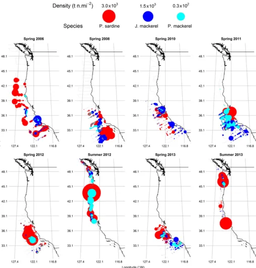
The periodic surveys performed since 2006 permit us to track the evolution of the most abundant epipelagic CPS in the CCE. The abundance of northern anchovy was not reliably estimated because in all years too few trawl samples included that species, indicating a degree of patchiness that is not well resolved with the large-scale sampling strategy needed for such large area. Also, the time series of herring abundance is too short and uncertain due to the lack of knowledge of the species habitat and spatial range, preventing conclusions about its population trajectory. On the other hand, the ATM-estimated abundances and distributions of sardine and mackerels allow evaluation of trends (Figures 5 and 6).

Since 2006, sardine dominated the CPS assemblage while exhibiting declining abundance (Figure 6) and a contracting distribution (Figure 5). These trends are the result of successive low recruitments since 2006 (Table 2). In 2011 and 2012, the sardine biomass increased temporar- ily due to a bolus of new recruits, but in 2013, both the spring and summer surveys indicated the lowest abundance of the time series.

While the sardine population declined from 2006 through 2011, the populations of both mackerels increased and their collective biomass surpassed that of sardine in 2011 (Figure 6). In 2011, mackerels of both species were abundant and in close proximity to the sardine (Figure 5).

In 2012 and 2013, mackerel abundances were lower than those in spring 2011. The combined biomass of epipelagic CPS in 2013 is the lowest since periodic ATM surveys started in 2006.

DISCUSSION

The ATM survey results from 2012 and 2013 show strong seasonal displacement in the distributions of the populations of sardine and mackerels between the offshore waters of Southern California and the coastal regions north of California, corroborating the existence of seasonal migrations in the CCE (Demer et al.,

2012). These migrations are probably synchronous across multiple species and perhaps in response to the same environmental cues. For sardine, the dynamics of their migratory behavior has been linked to the physical conditions, particularly the water temperature and chlorophyll-a concentration in the upper water column (Zwolinski et al., 2011; Demer et al., 2012). Attempts to characterize potential

habitats for Pacific and jack mackerel have been less definitive (Asch and Checkley, 2013). It is notable, however, that during both the 2012 and 2013 surveys, and during previous surveys (Demer et al., 2012, 2013; Zwolinski et al., 2012), mackerels were found both within and on the edge of the potential sardine habitat. This observation suggests that the seasonal migrations of jack and Pacific mackerel

TABLE 2. Acoustic-Trawl Method (ATM) survey estimates of biomass (million metric tons, Mt) for Pacific sardine (Sardinops sagax), jack mackerel (Trachurus symmetricus), Pacific mackerel (Scomber japonicus), northern anchovy (Engraulis mordax), and Pacific herring (Clupea pallasii) and their coefficient of variation (CV) and 95% confidence intervals (CI95%) for the 2006, 2008, 2010, 2011, 2012, and 2013 surveys. Note: Abundant CPS targets beyond the integration range in regions with Pacific herring suggest that the values presented here represent a small, but unknown, fraction of the stock. Future knowledge about the vertical distribution of the species will provide more accurate results.

Species Survey Biomass (Mt) CV (%) CI95% (Mt)

Pacific sardine (Sardinops sagax)

2006 Spring 1.947 30.4 0.897–3.139

2008 Spring 0.751 9.2 0.611–0.870

2010 Spring 0.357 43.3 0.094–0.690

2011 Spring 0.494 30.4 0.221–0.816

2012 Spring 0.469 28.6 0.224-0.750

2012 Summer 0.341 33.4 0.188–0.688

2013 Spring 0.305 24.4 0.167–0.454

2013 Summer 0.314 27.5 0.166-0.517

Jack mackerel (Trachurus trachurus)

2006 Spring 0.285 35.8 0.078–0.378

2008 Spring 0.147 28.4 0.075–0.232

2010 Spring 0.323 36.7 0.132–0.586

2011 Spring 0.389 34.0 0.157–0.650

2012 Spring 0.006 35.7 0.002–0.009

2012 Summer 0.097 23.4 0.053–0.140

2013 Spring 0.079 26.7 0.044–0.130

2013 Summer 0.009 54.0 0.002–0.020

Pacific mackerel (Scomber japonicus)

2006 Spring 0.047 61.6 0.006–0.109

2008 Spring 0.018 51.8 0.005–0.037

2010 Spring 0.018 45.7 0.001–0.034

2011 Spring 0.257 29.3 0.120–0.418

2012 Spring 0.014 53.2 0.005-0.031

2012 Summer 0.109 34.1 0.055–0.181

2013 Spring 0.013 31.5 0.005–0.019

2013 Summer 0.008 61.2 0.001–0.020

Pacific herring (Clupea pallasii)

2012 Summer 0.065 30.8 0.038–0.126

2013 Summer 0.050 28.3 0.024–0.085

(10)

are also linked with the environmental conditions that modulate sardine migration. Furthermore, it appears that the seasonal evolutions of the regional water masses are related to that of the transition zone chlorophyll front (TZCF). The TZCF is a band of water operationally defined as the 0.2 mg m^–3 surface chlorophyll-a isoline that separates sub-Arctic and subtropical waters. The front spans the entire North Pacific between 30°N and 45°N (Polovina et al., 2001; Bograd et al., 2004) and moves seasonally. Near North America, the 0.2 mg m^–3isoline inflects southward and runs parallel to the coast, extending as far south as Baja California (Figure 1). The potential habitat of the northern stock of Pacific sardine, roughly delimited offshore the 0.18 mg m^–3 and 15.4°C isolines (Zwolinski et al., 2011), is

typically located to the east and north of the TZCF. These two oceanographic indi- cators oscillate seasonally and simultane- ously, and may describe the same oceanographic dynamic (Bograd et al., 2004). We hypothesize here that the TZCF is related to the offshore and southern limit of both sardine and mackerel distributions, and that their juveniles might have nursery areas within the California Current, namely in the Southern California Bight, downstream of the main upwelling regions. In spring 2011 (Demer et al., 2013), for example, there were dense schools of small jack and Pacific mackerel offshore southern and central California.

While adult sardine migrate north during summer and fall and feed in the coastal waters, adult mackerels, predominantly piscivores, may occupy a larger offshore

and southern range to feed. The offshore presence of early life stages (Moser et al., 2001) and adult jack mackerel (MacCall and Stauffer, 1983; Macewicz and Hunter, 1993) suggest that they too migrate west and along the TZCF, similar to the behavior of highly migratory fishes like alba- core and yellowfin tunas and some bill- fishes such as marlin (Bograd et al., 2004;

PICES, 2004). Pacific mackerel, on the other hand, have a southerly distribution, probably extending to the southern tip of Baja California and into the Gulf of California (Fry and Roedel, 1949).

In contrast to sardine and mackerels, anchovy do not seem to migrate seasonally. Whether a species migrates or remains in an area may depend on its reproductive behavior and therefore its affinity to a particular oceanographic or seabed habitat. For example, sardine feed in the productive upwelling region off Oregon, Washington, and Vancouver Island in the summer; they batch spawn primarily in waters con- ducive to larval retention and growth located offshore of central and southern California during spring (Figure 4), and more rarely off Oregon and Washington (Lo et al., 2011). Anchovy also spawn off southern and central California during the winter, closer to the coast, and close to their coastal nursery regions, taking advantage of seasonal downwelling to increase retention of their eggs and larvae (Bakun and Parrish, 1982). Smelts and herring, in contrast, spawn in inter- tidal beaches (Love, 1996) and apparently have a stronger geographical fidelity. The forage fish in the CCE appear thus to be divided between sedentary and migrating species, each contributing in distinctive ways to the functioning of the ecosystem.

Migrating species such as sardine, mackerels, and hake exploit spatially segregated features of the system, striking a lucra- tive balance between somatic growth and energy storage during the feeding migration into productive northern waters and successful reproduction in the oligotrophic waters off southern California. With this life strategy, these species attain large

FIGURE 5. Spatial distributions and densities of Pacific sardine, jack mackerel, and Pacific mack- erel from 2006 through 2013. The summer surveys typically extend between Point Conception (California, USA) to the north end of Vancouver Island (Canada). The spring surveys generally occupy the region between the US/Mexico border to San Francisco.

(11)

biomasses during short periods of time and serve as large energy carriers that support communities of marine mammals, birds, and large migratory fishes (Field et al., 2001). Sedentary species, on the other hand, appear to attain lower biomasses but have important and sus- tained local effects on their suite of pred- ators (Willson et al., 2006). Management of the CPS ensemble requires both sus- taining local communities to ensure suf- ficient local forage as well as protecting migratory species from disruptions of their migrations, which could ultimately result in reduced fitness and even col- lapse, with harmful effects for the ecosystem (MacCall, 2012).

Ecosystem Sampling

Recruitment success for sardine and other CPS is strongly correlated to the environment (Zwolinski and Demer, 2014) and is highly variable. To manage stocks that are often dominated by a few strong year classes, surveys should be conducted once or twice per year. For sardine, the spring survey provides information about the spawning stock and their fecundity, and a summer survey may provide information about the age-0 recruits and the nutritional condition of migrating adults (Zwolinski and Demer, 2014). Fish ages, estimated from counts of otolith rings (Yaremko, 1996), may be used to convert the biomass-weighted length distributions to biomass-weighted age distributions of sardines (Zwolinski et al., 2009;

Demer et al., 2013). Surveying during spring, when sardine and mackerels are offshore and deeper in the water column, and then during summer, when they are near shore and in shallow waters, provide two independent estimates of abundance and seasonal distribution for each target population. In the case of the sardine, the two time series have been providing valuable information for the annual stock assessments (Hill et al., 2014).

Despite the advantages of ATM surveys, improvements to the current methods are warranted. For example, efforts should be made to characterize the

three-dimensional habitats of the most abundant species, using a combination of direct and remote observations of the fishes and of their surrounding environment. The sampling strategy should be improved for species that reside in offshore and in deep water, and near the coast and in shallow water. For stocks that span the Exclusive Economic Zones of multiple countries, multinational (e.g., Mexico, United States, and Canada) collaboration is needed to synoptically sample the entire CCE. Also, methods should be further developed to use data from wide bandwidth echosounders (e.g., Simrad EK80) to better clas- sify backscatter to species, perhaps inde- pendently of the trawl catches.

In addition to sampling the epipelagic fishes that are periodically abundant, the ATM surveys can sample multiple other important taxa in the CCE. In particular, efforts are being finalized to routinely provide estimates of euphausiids, important prey for many fish species, in a manner similar to that used for fish (Hewitt and Demer, 1994; Demer, 2004). Salps, pyro- somes, and jellyfishes can attain extremely large abundances over short periods, and such “blooms” can potentially harm the

productivity of species having pelagic eggs and larvae (Lynam et al., 2006). These gelatinous organisms can also be observed and quantified acoustically (Hewitt and Demer, 1994; Wiebe et al., 2010; Graham et al., 2010). ATM estimates of their abundances and distributions should provide information for understanding predator- induced variability in the recruitment of many CPS species.

ATM surveys can be the backbone of ecosystem surveys when augmented with concurrent measurements and observations of physical oceanography, phytoplankton, zooplankton, ichthyoplankton, highly migratory fish species, seabirds, and marine mammals. Many of these samples are or could be collected while underway during the acoustic surveys.

Sea surface temperature, salinity, and chlorophyll-a concentration are sampled continuously in the near surface through- out each survey using thermosalinograph and fluorometer instruments. CTD pro- files are collected using a probe deployed and retrieved from the ship’s stern without stopping, and regularly spaced deep oceanographic stations can be made for in-depth analysis. A continuous underway fish-egg sampler (CUFES) pumps

FIGURE 6. Time series of Pacific sardine and mackerels (jack and Pacific mackerel combined), and their sum with respective 95% confidence intervals, as estimated from acoustic-trawl method (ATM) surveys. The sum of epipelagic CPS dropped to a study-period minimum in 2013.

(12)

water through the ship’s hull and sieves ichthyoplankton and zooplankton that are periodically counted and identified to species (Checkley et al., 1997). These data provide qualitative information about the presence of spawning fish, by species.

The sardine eggs counts are used to routinely verify the predicted potential sardine habitat. Periodic samples of plankton in the water column, using either single- or multiple- opening-and-closing nets for vertically stratified sampling, provide information on the habitat and the distribution of food for planktivores and pred- ators. Towed undulating underway optical plankton counters (Herman, 1988) can resolve planktonic particles larger than 0.25 mm, thereby increasing the volume filtered by the above samplers by an order of magnitude. Likewise, optical net systems can be used to estimate, in real time, the species and size composition of fish schools sampled acoustically. Passive acoustic systems can be used concurrently to obtain the locations and source levels of marine mammal calls, which can then be used to direct computer-controlled recognition cameras to provide images of mammal aggregations. With the rapid increase of satellite-based bandwidth, many of the operations described here can be controlled remotely from shore, freeing valuable space on the ships for scientists conducting in situ experiments and physical sampling.

CONCLUSION

The physicochemical and biological environment in the CCE varies on multiple scales and appears to drive the distributions, abundances, and species dominance of epipelagic CPS, in particular sardine, anchovy, and mackerels.

Advances in fisheries acoustics and periodic ATM surveys, coupled with in situ and remote sensing of the environment and other trophic levels, provide an efficient and practical means to empirically assess multiple CPS in the context of each other and their biotic and abiotic environments. The results from future surveys will expand further to include the

distributions, abundances, and perhaps potential habitats of other CPS, euphausiids, and gelatinous organisms, as well as concurrent underway measures of physical oceanography, ichthyoplankton and phytoplankton, highly migratory fishes, seabirds, and marine mammals.

ACKNOWLEDGEMENTS. We thank Brian Elliot, Scott Mau, David Murfin, Josiah Renfree, and Steve Sessions for their contributions to the acoustic sampling and data processing, and David Griffith, Amy Hays, Sherri Charter, Sue Manion, Bill Watson, and others from the SWFSC for collecting and processing the trawl and plankton samples. We thank Russ Vetter, Bill Watson, and Andrew Thompson, from the SWFSC, and two anonymous reviewers for their constructive critiques of this work. This article does not necessar- ily reflect the official views or policies of the National Marine Fisheries Service, the National Oceanic and Atmospheric Administration, the Department of Commerce, or the Administration.

REFERENCES

Agostini, V.N., R.C. Francis, A.B. Hollowed,

S.D. Pierce, C. Wilson, and A.N. Hendrix. 2006. The relationship between Pacific hake (Merluccius pro- ductus) distribution and poleward subsurface flow in the California Current System. Canadian Journal of Fisheries and Aquatic Science 63:2,648–2,659, http://dx.doi.org/10.1139/f06-139.

Alheit, J., and A. Bakun. 2010. Population synchronies within and between ocean basins: Apparent tele- connections and implications as to physical-biological linkage mechanisms. Journal of Marine Systems 79:267–285, http://dx.doi.org/10.1016/

j.jmarsys.2008.11.029.

Asch, R.G., and D.M. Checkley. 2013. Dynamic height: A key variable for identifying the spawning habitat of small pelagic fishes. Deep Sea Research Part I 71:79–91, http://dx.doi.org/10.1016/

j.dsr.2012.08.006.

Bakun, A., and R.H. Parrish. 1982. Turbulence, trans- port, and pelagic fish in the California and Peru current systems. California Cooperative Oceanic Fisheries Investigations Reports 23:99–112.

Barange, M., I. Hampton, and M. Soule. 1996.

Empirical determination of in situ target strengths of three loosely aggregated pelagic fish species. ICES Journal of Marine Science 53:225–232, http://dx.doi.org/10.1006/jmsc.1996.0026.

Baumgartner, T., A. Soutar, and V. Ferreira-Bartrina.

1992. Reconstruction of the history of pacific sardine and northern anchovy populations over the past two millennia from sediments of the Santa Barbara Basin, California. California Cooperative Oceanic Fisheries Investigations Reports 33:24–40.

Bograd, S.J., D.G. Foley, F.B. Schwing, C. Wilson, R.M. Laurs, J.J. Polovina, E.A. Howell, and R.E. Brainard. 2004. On the seasonal and interan- nual migrations of the transition zone chlorophyll front. Geophysical Research Letters 31, L17204, http://dx.doi.org/10.1029/2004GL020637.

Checkley, D.M., P.B. Ortner, L.R. Settle, and S.R. Cummings. 1997. A continuous, underway fish egg sampler. Fisheries Oceanography 6:58–73, http://dx.doi.org/10.1046/j.1365-2419.1997.00030.x.

Cutter, G.R. Jr., and D.A. Demer. 2008. California current ecosystem survey 2006. Acoustic Cruise Reports for NOAA FSV Oscar Dyson and NOAA FRV David Starr Jordan. NOAA Technical Memorandum NMFS-SWFSC-415, 98 pp.

Demer, D.A. 2004. An estimate of error for the CCAMLR 2000 survey estimate of krill biomass. Deep Sea Research Part II 51:1,237–1,251, http://dx.doi.org/10.1016/j.dsr2.2004.06.012.

Demer, D.A. 2012. 2007 Survey of Rockfishes in the Southern California Bight Using the Collaborative Optical-Acoustic Survey Technique. US Department of Commerce, NOAA Technical Memorandum, NOAA-SWFSC-498,110 pp.

Demer, D.A., G.R. Cutter, J.S. Renfree, and J.L. Butler. 2009a. A statistical-spectral method for echo classification. ICES Journal of Marine Science 66:1,081–1,090, http://dx.doi.org/10.1093/

icesjms/fsp054.

Demer, D.A., R.J. Kloser, D.N. MacLennan, and E. Ona.

2009b. An introduction to the proceedings and a synthesis of the 2008 ICES Symposium on the Ecosystem Approach with Fisheries Acoustics and Complementary Technologies (SEAFACTS).

ICES Journal of Marine Science 66:961–965, http://dx.doi.org/10.1093/icesjms/fsp146.

Demer, D.A., J.P. Zwolinski, K. Byers, G.R. Cutter Jr., J.S. Renfree, S.T. Sessions, and B.J. Macewicz.

2012. Prediction and confirmation of seasonal migration of Pacific sardine (Sardinops sagax) in the California Current ecosystem. Fisheries Bulletin 110:52–70, http://fishbull.noaa.gov/1101/

demer.pdf.

Demer, D.A., J.P. Zwolinski, G.R. Cutter Jr., K.A. Byers, B.J. Macewicz, and K. Hill. 2013. Sampling selec- tivity in acoustic-trawl surveys of Pacific sardine (Sardinops sagax) biomass and length distribution.

ICES Journal of Marine Science 70:1,369–1,377, http://dx.doi.org/10.1093/icesjms/fst116.

Efron, B. 1981. Nonparametric standard errors and confidence intervals. Canadian Journal of Statistics 9:139–172.

FAO (Food and Agriculture Organization of the United Nations). 2003. Fisheries Management:

The Ecosystem Approach to Fisheries. FAO Technical Guidelines for Responsible Fisheries No. 4, Suppl. 2, 112 pp.

FAO. 2012. The State of World Fisheries and Aquaculture. FAO Fisheries and Aquaculture Department, Rome, http://www.fao.org/docrep/016/

i2727e/i2727e00.htm.

Field, J.C., R.C. Francis, and A. Strom. 2001. Toward a fisheries ecosystem plan for the northern California Current. California Cooperative Oceanic Fisheries Investigations Reports 42:74–87.

Finney, B.P., I. Gregory-Eaves, M.S.V. Douglas, and J.P. Smol. 2002. Fisheries productivity in the northeastern Pacific Ocean over the past 2,200 years. Nature 416:729–733, http://dx.doi.org/

10.1038/416729a.

Foote, K.G. 1980. Importance of the swimbladder in acoustic scattering by fish: A comparison of gadoid and mackerel target strengths. Journal of the Acoustical Society of America 67:2,084–2,089, http://dx.doi.org/10.1121/1.384452.

Foote, K.G. 1983. Linearity of fisheries acoustics, with additional theorems. Journal of the Acoustical Society of America 73:1,932–1,940, http://dx.doi.org/ 10.1121/1.389583.

Foote, K.G., F.R. Knudsen, G. Vestnes, D.N. MacLennan, and E.J. Simmonds. 1987.

Calibration of Acoustic Instruments for Fish Density Estimates: A Practical Guide. ICES Cooperative Research Report No. 144, 81 pp.

Fry, D.H. Jr., and P.M. Roedel. 1949. Tagging Experiments on the Pacific Mackerel (Pneumato- phorus diego). State of California Department of Natural Resources, Fish Bulletin 73, 67 pp, http://www.escholarship.org/uc/item/33t588wf.