Decay
Author(s)
Miyagi, Hayao
Citation
琉球大学工学部紀要(24): 103-111
Issue Date
1982-09
URL
http://hdl.handle.net/20.500.12000/5590
Bull. Faculty of Engineering., Univ. of the Ryukyus, No. 24, 1982. 103 Transient Stability of the Power System
with the Effect of Flux Decay Hayao MlYAGI*
Summary
In this paper, the transient stability of the single-machine system with the effect of flux decay is studied. The Lagrange-Charpit meth od is used for the construction of the Lyapunov function for stability study of the power system. A product-type nonlinearity depending on flux decay is well-defined. The positive definiteness of the ob tained Lyapunov function and the negative semi - definiteness of its time derivative are easily verified in the region which satisfy the sec tor-condition of this nonlinearity. The stability boundaries given by the proposed Lyapunov function are compared with those obtained by
conventional Lyapunov function.
Key words : Power system, Stability, Lyapunov method. List of principal symbols
M = machine inertia in p.u. power second2 per electrical radian.
D = machine damping coefficient in p.u. power-second per electrical radian.
Pt = mechanical power input, p.u.. PE = electrical power output, p.u..
Eex = exciter voltage referred to the armature circuit, p.u.. EB = voltage of infinite bus, p.u..
E'q = voltage proportional to field flux linkage, p.u.. xd = direct axis synchronous reactance, p.u..
x 'd = direct axis transient reactance, p.u..
xl2 = total reactance between the generator terminal and the infinite
bus, p.u..
T'o = open circuit transient time constant, s.
e = value of E' at the prefault stable equilibrium point. $ = angle in radians between EB and E'q.
§o = value of 6 at the prefault stable equilibrium point. / = generator current.
Received : April 30, 1982
!04 with the Effect of Flux Decay:MIYAGI Id =d-component of /.
1 .Introduction
The effect of flux decay on the transient stability of a synchronous machine has been
investigated by many authors, using the direct method of Lyapunov. Thus, various meth ods have been used to construct Lyapunov functions. Siddiqee developed a Lyapunov function by trials based on physical consideration . Afterwards some techniques were
used in attempts to improve Siddiqee's function. Among them are (a) variable gradient
technique2^, (b) Initiating function technique 3) and (c) Kalman's procedure under Desoer
-Wu's condition 4\ However, all of the resulting Lyapunov functions by these techniques
are equivalent to the energy function developed by Siddiqee. Those techniques could not
deal with the product-type nonlinearity well. This difficulty is due to violation of the sector condition of such nonlinearity which exists in generator output.
In a recent paper, the author has presented the Lagrange - Charpit method5^ of con
structing Lyapunov functions for power systems. This method determines the arbitrary
non-negative function $ which allows the Lyapunov function to be determined.
This method is applied to a synchronous machine with the effect of flux decay in
this paper. Aforementioned difficulty is overcome through both the Lagrange - Charpit ap proach and some arrangement of the nonlinearity. Hence, a new Lyapunov function can be derived. Furthermore, the positive definiteness of the obtained Lyapunov function and
the negative semi - definiteness of its time derivative can be easily verified in the region
which satisfy the sector - condition of this nonlinearity.
A summary of the Lagrange - Charpit method is given in the following section. 2 . Lagrange -Charpit method
Consider a nonlinear autonomous system represented by
i = / O), / (o) = o (1)
where x is the n-vector, / (jr) is the n-vector function and x = o is the equilibri um state which is asymptotically stable. A candidate Lyapunov function is obtained by
solving
F O, V, P) = PT f O) + <f> O) = 0
(2)
where P = dV/dx and 0 (jr) is an arbitrary non-negative function whose opposite sign becomes the time derivative of the obtained Lyapunov function.
The characteristic equation for eqn. 2 is given by
dxl dx2 dxn
Bvll. Faculty of Engineering., Univ. of the Ryukyus, No. 24, 1982. 105 dv dF dF — + P2 — + 4- P dP P
V dPn
-dP, -dP, -dPm d2F + P2dvF dnF +PndyF (3)where dnF=QF/dxn and 8VF= QF/QV and dxF, dsF, ... , dnF include dx$, d2fr ... ,
dB$, respectively.
If we can obtain equations containing at least one component of P from eqn. 3, such that
G, O, V, P, d$/dx) = 0
r, V, P, =0
(?„_, (jt, V, P, =0
(4)
then, in order for .F and C to have a common solution, these functions must satisfy the
conditions
tK dxk dPk
dxk dPk
(5)where i = 1, 2, ... , ra-1.
If [G,-, F~\ still give partial differential equations including P, they must also have a common solution with F. Hence, we let [G,-, F~] = G once again. These manipula tions are continued until the 2nd-order partial differential equations for $ are given, be
cause we would like <t> to be in a quadratic form so that its positive semi-definiteness can
be easily verified. Thus the unknown d$/dx and $ are determined from the conditions
[G., G,] = dGr dG. dG. dGr —-dxk dPk dxk QPk n . dG. dF dF dG. .
te dP dxk 8P J
=0 (6)where r,s = 1,2,..., max [i], and
dGr = 9Gr | p dGr
dxk
dxk
k dV
From the conditions §,d$/dx and <f> can be expressed by using x.
If eqns. 2 and 4 can be solved so as to give P as the function of x and V as
(7)
the Pfaffian differential equation
PTdx = (JVfdx
is integrable. Hence, a possible Lyapunov function and its time derivative are
(9) V Car) - v o rx = PT ^o dx (10)
3. Formulation of the problem
Neglecting resistance and transient saliency, the dynamic equations of a single-ma chine connected to an infinite - bus, taking into consideration of the flux decay are given
by d2d dt
=J_r
T' L
- x 'd ) ld - E' wherePE =
sin 8 xDefining state variable as *i = d -d0
x2 = 8
x3 = E'g - e
we can represent the system as follows : xl x2 _ x3 _ =
" /l
k
./.
(*)■
(*) where Vi = = cos 80 - cos(xx + xd)T0 'q - EB cos 8 V2 =(Xd ~ X'd )EB
(x12 + x'd)T'o (11) (12) (13)Bull. Faculty of Engineering., Univ. of the Ryukyvs, No. 24, 1982. 107
4. Construction of Lyapunov function
A scalar function V is obtained as a function which satisfies the linear partial differ ential equation given by eqn. 2. The characteristic equation then becomes
dx. dx, dV
-dP1 -dP2 _ -dP3 82F
From the above equation, we obtain
(14) ax2 - Cj (x3 + e) sin(xx 'P -Px r(xx)x2 -£ (Vlx3 4- 772^(^1 dP, (15) sin (x,
4-where a,fi,£ are arbitrary constants and yix^ is an arbitrary function. Integrating the numerators, we obtain
G, = -Pi = 0
-Pz=0 (16)
where
and then the following two equations must be satisfied;
G3 =ax2 -p \Dx2 4- K} (x3 +e) sin ( + i» - (J)/M)P2 + d<f>/dx2 = = r(xi)x2 -, -P2 sin(xx 4-(17)
where G3 and G4 coincide with [GtJ F] and [G2, -F], respectively. Then the application of eqn. 6 to [Git i= 1-4} and F gives
[Glf G2] = 0
[G,, G3] =2{ct-} ^
Bull. Faculty of Engineering., Univ. of the Ryukyus, No. 24,1982 109
Px = a* (D/M)x2 + a' (D/M? + {K, (x3 + e) sin{xl + d0)
-+ 2{D/M)/a> (l-tfOx.^x,)
P3 =Hence, the scalar function V is given by eqn. 10 as
D K ( /-— r—— y
-2 ■r2+«'M-ri) + 2M y~8iXi)+J~X3 j
+-«' (i-d/)(—)2x2 +2— /a' (1-a'
2 A/T l M V(22)
(23)
To inspect the definiteness of V, we rewrite the right-hand side of eqn. 23, except the first and second terms, such that
(24) where H (x{)= a' sin2 As we can write sin2 - [(D/M) sin2 (25)
the sector - condition x{ Hix^) ^ 0 can be verified in the neighbourhood of the origin.
Then Vj is a non-negative function around the origin. Hence, V" given by eqn. 23 is a positive definite function.
no with the Effect of Flux Decay: MIYAGI
v
Vi
V2
S
1
~M
(26)which is the equivalent function given by references 1, 3, 4 and 5.
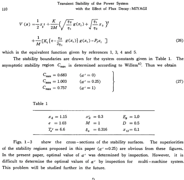
The stability boundaries are drawn for the system constants given in Table 1. The
asymptotic stability region Cmax is determined according to Willem6 . Thus we obtain
Cmax = 0.683 Cmax = 1.003
Qnax = 0.757
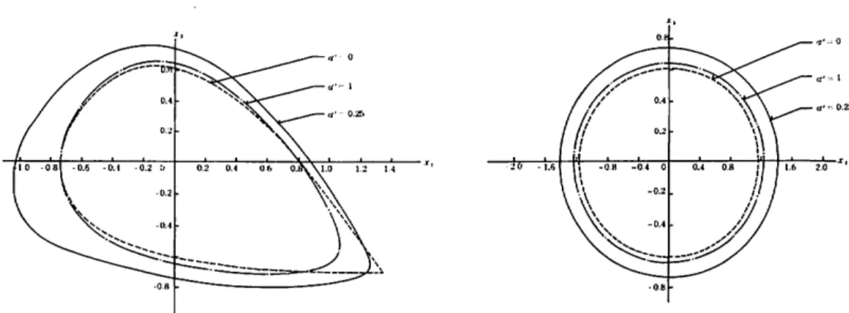
ice' -0.25) (27) Table 1 xd = 1.15 e = 1.03 V = 6.6 M So = 0.3 = 1 = 0.316 EB D *,: = 1.0 = 0.5 2= 0.1Figs. 1-3 show the cross - sections of the stability surfaces. The superiorities
of the stability regions proposed in this paper (#' =0.25) are obvious from these figures. In the present paper, optimal value of a' was determined by inspection. However, it is difficult to determine the optimal values of a' by inspection for multi - machine system.
This problem will be studied further in the future.
1.0 -0.8\ —0.6 -0.4 —0.2 0
-1.6
Bvll. Faculty of Engineering., Univ. of the Ryukyus, No. 24, 1982. Ill
Fig. 2: Cross - sections of stability surfaces
in the plane x2 = 0
Fig. 3: Cross - sections of stability surfaces in the plane x i = 0 5. Conclusion
The transient stability of the single-machine system with the effect of flux decay
has been studied. The Lagrange-Charpit method is applied to construct Lyapunov func tion. The conventional energy function is a special case of the Lyapunov function pro posed in this paper.
Numerical examples show that the proposed Lyapunov function gives better estima
tion of stability boundary than those currently available.
The application to the system with effects of flux decay and AVR action will be dis cussed on another occasion.
References
1. M. W. Siddiqee : ' Transient stability of an A. C. generator by Lyapunov's direct method',
Int. J. Control, 1968, 8-2, pp. 131-144.
2. A. K. De Sarkar and N. Dharma Rao : 'Zubov's method and transient-stability problems
of power systems', Proc. IEE, 1971, 118-8, pp. 1035-1040.
3. T. K. Mukherjee and B. Bhattacharyya :'Transient stability of a power system by the sec ond method of Lyapunov', Int. J. Systems Sci., 1972, 3-4, pp. 439-448.
4. M. A. Pai and Vishwanatta Rai:'Lyapunov-Popov stability analysis of synchronous ma chine with flux decay and voltage regulator', Int. J. Control, 1974, 19-4, pp. 817-829. 5. H. Miyagi and T. Taniguchi :'Lagrange - Charpit method and stability problem of power
systems', Proc. IEE, 1981, 128-3, pp. 117-122.
6. J. L. Willem :'The computation of finite stability regions by means of open Lyapunov sur