トップページ北見工業大学学術機関リポジトリ（KITR） LIDYANA 学位論文

(1)

El as t o- pl as t i c def or m

at i on anal ys es of t he

i nt er ac t i on of c ol ony s t r uc t ur es i n t he

m

i c r os t r uc t ur e of pear l i t e s t eel s

その他のタイトル

（パーライト鋼の微視組織におけるコロニー間の相

互作用に関する弾塑性変形解析）

著者

LI D

YAN

A BI N

TI RO

SLAN

学位名

博士（工学）

学位授与機関

北見工業大学

学位授与番号

10106甲第156号

研究科・専攻名

生産基盤工学専攻

学位授与年月日

2017- 03- 17

(2)

博

士

論

文

Doctoral Thesis

(パ鋼微視組織けコロ間相互作用関弾塑性変形解析)

Elasto-plastic deformation analyses of the interaction of

colony structures in the microstructure of pearlite steels

2017

3 2017

March

(3)

(4)

要旨

パ鋼強度靱性優，橋梁ケワ構

造材料広く利用さい．そ優性質パ鋼微視組織

来．パ鋼微視組織，高強度あ脆いン

強度あ延性を持ェ交互積層構造あ．ン

層配向方向領域をコロ言い，パ鋼微視組織多

数コロ構成さい．パ鋼強度積層構造影響さ，

延性コロ構造影響さこ実験知．わ，

サクロン寸法ェ高い応力を担う一方，コロ中ン

塑性変形いこ観察さ．，こうこ生

体的十分解明さいい．本研究，積層構造を

持コロ弾塑性変形詳細を検討．

パ鋼弾塑性変形古的弾塑性論基い限要素法を用

い解析．こ研究，体ンェ積層

，ン層内生ひ応力集中抑制さ，ン

塑性変形安定こ分．ェ層寸法サクロ

(5)

構造，隣接いコロ内積層配向方向組合わ，

コロ界面近傍やコロ内生ひ異こ分．実

験コロ配向方向表面観察い，う配向方向

を持コロひ分布異場合あ理十分説明い．

近，コロ三次元的構造観察さ，奥行方向傾いいン

層確認．

本研究，二次元三次元コロを構築，そ変形を解析

．そ結果，ェ加工硬能塑性流動応力高くン

塑性変形を安定こ分．，積層方向引張方向

行あ，コロ塑性流動応力最高く，引張方向 45ま傾く

，塑性流動応力最く．わ，積層配向方向体コロ

変形特性大く影響．積層配向方向，コロ変形

異方性生方大く異．隣接いコロ塑性流動応力差

高い場合く変形異方性違いコロ界面ひ応力

集中生こ確認．，コロ構造集合体あパ

鋼微視組織弾塑性変形コロ間相互作用影響さこ分

(6)

ABSTRACT

Pearlite steels are widely used in construction structures, vehicles or other

engineered productions alike because pearlite steels exhibit both high strength and

toughness. The microstructure contributes to the outstanding characteristics. The

microstructure is lamellar structures consist of alternately layered high-strength but

brittle cementite and low-strength but ductile ferrite. A region where the cementite

lamellae aligned in the same direction is called ‘colony’. Thus, a pearlite microstructure

is a map of variously oriented colony structures. Experiments have proven that the

strength of pearlite depends on the lamellar structures and the ductility depends on the

colony structures. Specifically, sub-micron size ferrite is capable of bearing higher

stress; while cementite within colonies is observed to deform plastically. However,

the details of the mechanisms behind these abilities are still unclarified. For that, we

study the details of the elasto-plastic deformation of colonies which are constructed

from lamellar structures.

Elasto-plastic deformation of the pearlite steel is analysed by finite element method

that employs the classical elasto-plastic theory. From previous studies, we learned that

the increased numbers of lamellar suppress the concentration of strain and stress in

cementite lamella which leads to the stability of cementite's plastic deformation. On top

of that, ferrite also contributes to the stability of cementite's plastic deformation when

the size is in sub-micron order. In colony structures, the difference of lamellar

alignments of neighbouring colonies influences the distribution of strain around the

(7)

these deformations from the surface of the specimens. Hence, detailed explanations why

different distributions of strain occur between colonies with similar lamellar are yet to

be elucidated. Recently, the three-dimensional structure of colonies which confirm the

transversal inclination of cementite layer has been observed.

For this study, we construct two-dimensional and three-dimensional colony models

and analyse the deformation. The results show that the plastic deformation of cementite

stabilised when the strain-hardening rate and plastic flow of ferrite are high. Next, when

the colony alignment is parallel to the tensile direction, the plastic flow stress of the

colony is the highest. Meanwhile, when the colony alignment is 45 inclined towards

the tensile direction, the plastic flow stress is the lowest. In other words, the lamellar

alignment of the single-colony models significantly influences the behaviour of its

deformation. Likewise, the lamellar alignment of the colony controls the anisotropy of

the single-colony models. Concentrations of strain and stress around colony

boundaries confirmed when the difference of plastic flow stress between two adjacent

colonies is high or/and the anisotropic difference is prominent. Therefore, the

elasto-plastic deformation in an assembly of colony structures such as pearlite

(8)

List of figures

Chapter 1 Overview

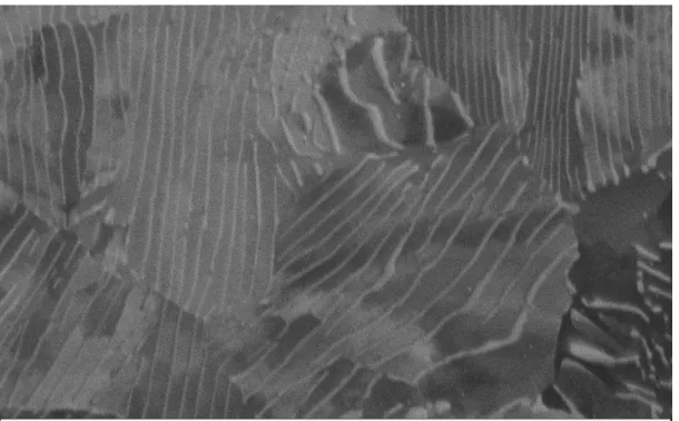
Fig. 1 SEM photo of microstructure in as-patented pearlite [36]. 3

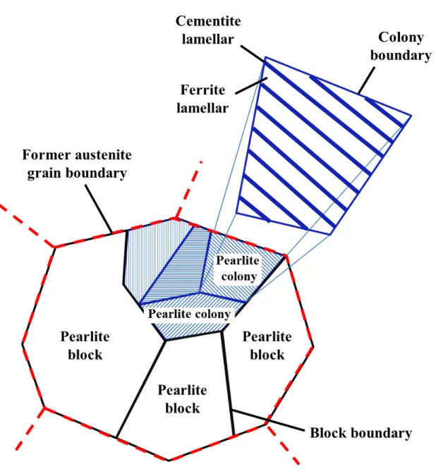
Fig. 2 Schematic diagram of the pearlite microstructure. The description explains

the relative hierarchy of pearlite substructures: the pearlite block structure,

the pearlite colony structure and the pearlite lamellar structure which

consisted of alternate layer of cementite and ferrite lamellae [36]. 4

Fig. 3 Distribution of equivalent strain, eq in two adjacent colonies at nominal

strain _o 18%. The angle between the lamellar alignment is denoted as

. The grey arrows indicate the tensile direction [62].

8

Fig. 4 Distribution of plastic strain pl propagation at drawing strain  5%

around block/colony boundaries. (a) and (b) show three colonies with similar

lamellar arrangement: a triple point meet. The dotted lines and arrows

represent block/colony boundaries and lamellar alignment of cementite

respectfully [36].

9

Chapter 2 Analyses condition

Fig. 5 Stress-strain curve of typical mild steel under uniaxial tensile deformation. 16

Fig. 6 Idealisation of elasto-plastic deformation. (a) Elastic-perfect plastic material,

and (b) power plastic hardening material.

22

Fig. 7 Stress-strain curves for cementite and ferrite. 23

Fig. 8 Stress-strain curve for true and nominal curve for cementite. This

figure shows the plastic flow stress for elastic-perfect plastic material stress established for cementite in comparison to the simulation data.

26

Fig. 9 Diagram of the von Mises yield condition in the principal stress space. 29 Fig. 10 The relationship between yield surface and strain increment. 30

Chapter 3 Modelling of pearlite colony

Fig. 11 Basic types of the morphology of cementite in pearlite microstructure. 34

Fig. 12 Schematic of 2-D orthogonal projection and 3-D view of a pearlite colony. (a)

is the orthogonal projection of cementite ( ) and ferrite () lamellar. (b) The direction of the  plane is determined by the direction of normal vector, n. The direction of n is determined by the azimuthal angle at the

(11)

xy-plane,



and the inclination angle from z-axis,  of the  plane in 3-Dspace.

Chapter 4 Elasto-plastic deformation of single-colony models

Fig. 13 Schematic of five-layered pearlite model. The indentation at the mid-section

of the central cementite is a cosine function. It is fixed along the x-axis at the

left lateral surface, while forced displacement is given at the right lateral

surface. The illustration is exaggerated.

41

Fig. 14

True stress _tr vs. plastic strain pl curves to compare Ferrite-org and

the hypothetical Ferrite5, Ferrite 10 and Ferrite 5n500.  is a constant.

43

Fig. 15 Distribution of tensile plastic component _xxpl at nominal strain

1.529% o

  in model (a) ferrite-org (low flow stress, low hardening rate, (b) Ferrite5n500 (high flow stress, low hardening rate) , (c) Ferrite5 (high

flow stress, high hardening rate), and (d) Ferrite10 (high flow stress, high

hardening rate).

45

Fig. 16 Distribution of tensile stress component xx at nominal strain

1.529% o

  in model (a) Ferrite-org (low flow stress, low hardening rate, (b) Ferrite5n500 (high flow stress, low hardening rate) , (c) Ferrite5 (high

flow stress, high hardening rate), and (d) Ferrite10 (high flow stress, high

hardening rate).

46

Fig. 17 The nominal stress o versus nominal strain o curves of bulk cementite

and three-layered lamellar structure models.

47

Fig. 18 Schematic of a single-colony structure. Cementite lamellar is denoted as 

plane. The alignment of  plane depends on the direction of normal vector,

n which is determined by angle  and  . The schematic also defines the

boundary conditions.

49

Fig. 19 Diagram of pearlite single-colony models. The dimension of the models are

L L L  . The thickness of the colony boundary, ferrite lamellae () and cementite lamellae ( ) are L15.The alignment of  is inclined at

inclination angle  first, then  .

50

Fig. 20 Propagation of equivalent strain eq in single-colony models at nominal

strain _o 1.5% and _o3%.

54

Fig. 21

Distribution of equivalent plastic strain _eqpl and plastic tensile strain

component _xxpl in single-colony models at nominal strain _o3%.

(12)

Fig. 22

Distribution of equivalent elastic strain _eqel in single-colony models at

nominal strain _o3%.

56

Fig. 23

Distribution of total normal strain component t_yy and total transverse

strain component t_zz in single-colony models at nominal strain _o3%. 57

Fig. 24

Distribution of total shear strain components t xy

 , t yz

 and t zx

 in

single-colony models at nominal strain _o3%. Here x-, y-, and z-axes are

tensile, normal and transverse axes. The surface of xy is the longitude

surface and zx is the horizontal surface. They are parallel to the tensile

direction. yz is the transverse surface normal to the tensile direction.

59

Fig. 25

Distribution of equivalent stress _eq at nominal strain _o 3% shown in

separate stress gauges that accommodate both stress ranges for  and



phases. The stress are denoted as _eq and _eq respectively.

61

Fig. 26 The nominal stress o vs. nominal strain o curves of single-colony

models in comparison with monolithic  and .

63

Chapter 5 Elasto-plastic deformation of multi-colony models

Fig. 27 SEM of three-types of block/colony regions taken at strain [36] and their 2-D

schematics. The boundary conditions are defined at both lateral surfaces. 67

Fig. 28 The upper row shows the distribution of plastic strain pl in experimental specimens at strain  5%. The lower row shows the distribution of plastic tensile strain component _xxpl for FEM analyses results at nominal strain

5%,10%,13%

o

  and 15% for model-(a), -(b), and -(c).

70

Chapter 6

Fig. 29 Schematic of 2-D double-colony model. The model parameter is L2L. The

double-colony is divided into Colony1 (C1) and Colony2 (C2) at the colony

boundary (CB). The lamellar alignment in C1 is perpendicular to the tensile

axis (x-axis) while C2 inclines at the angle of  from C1. The thickness

ratio of



to  is d 2

d   

; given that

11

L

d_  . The left lateral surface

is constrained, and the right lateral surface is given forced displacements.

(13)

Fig. 30 Distribution of plastic tensile strain component _xxpl in 2-D double-colony

models at nominal strain _o5%,10%,13% and18% . The angle of

difference between  alignments in C1 and C2 are   30 , 45 and60.

75

Fig. 31 Diagram of pearlite 3-D double-colony models. Colony1 (C1) and Colony2

(C2) are joined at the colony boundary (CB). The dimension of the model is

2L L L  2. The thickness of CB, , and  are L10. The alignment of

 in C2 is fixed. The alignment of  in C1 is inclined at inclination angle

 first, then  .

78

Fig. 32 Diagram of pearlite double-colony models. The dimension of the model is

2L L L  2. The thickness of CB,  and , are L10.The alignment of

 in C2 is fixed at _o135. The alignment of  in C1 is inclined at inclination angle  first, then  .

79

Fig. 33 Development of equivalent strain eq in pearlite double-colony models at

nominal strain _o 1.5% and _o3%.

82

Fig. 34

Distribution of equivalent plastic strain _eqpl and plastic tensile strain

component_xxp at nominal strain _o3%.

83

Fig. 35

Distribution of total normal strain component, t_yy and total transversal

strain component, t_zz at nominal strain _o 3%.

85

Fig. 36

Distribution of total shear component for _xyt , t_yz and _zxt at nominal

strain_o3%.

87

Fig. 37

Distribution of total yz strain component t_yz at cross sections of C1, CB

and C2 for model-(b) and model-(e) at nominal strain _o3%.

89

Fig. 38

Distribution of total yz strain component t_yz at cross sections of C1, CB

and C2 for model-(f) and model-(g) at nominal strain _o 3%.

90

Fig. 39

Distribution of equivalent stress _eq at nominal strain _o 3%. Stress

ranges are arranged for each  and  are denoted as _eq and _eq

respectively.

93

Fig. 40 The nominal stress o vs. nominal strain o curves of double-colony

models.

(14)

Chapter 7 Discussion

Fig. 41 Distribution of stress components in single-colony models. 99

Fig. 42 The relationship between average equivalent plastic strain and  lamellar

alignment towards the tensile direction [36].

102

List of table

Chapter 4 Elasto-plastic deformation of single-colony models

(15)

(16)

Chapter 1 Overview

1

Chapter 1 Overview

1.1 Introduction

In 1881, Sorby [1] discovered “the pearlycompound” which is later widely known

as “Pearlite”. Pearlite is a type of eutectoid steel. It is the product of austenite

decomposition [2-8] from heat treatment and subsequent cooling process. The patenting

process transforms austenite into a lamellar structure consisting of high-strength yet

brittle cementite and low-strength yet ductile ferrite phases [9,10]. Managing the

annealing process of patenting allows manufacturers to control the strength and

toughness of pearlite during the wire-making process [11-15]. Thus the applications of

pearlite steels range from piano strings to steel cords found in vehicle tires and cable

wires of suspension bridges [15-18]. The brittle/ductile lamellar structure allows

trade-off attributes of high strength and ductility to complement each other [19-29]. To

date, pearlite steel exhibits the greatest strength amongst mass-produced wire materials

(17)

2

1.2 Pearlite microstructure

Hull and Mehl [9] mentioned that Belaiew [32] initially described the pearlite

colony by assuming that the cementite lamellae were arranged parallel with each other

in the ferrite matrix –where they were thought to have obliged a certain crystallographic

orientation. However, this orientation was considered to be different from the original

austenite crystallographic orientation. Mehl and Smith [33] studied the case [32] and

found that the original austenite predetermined the orientation of ferrite. Jolivet [34]

observed that a pearlite nodule consisted of zones (colonies) where ferrite and cementite

lamellae were alternately layered while lying parallel along a particular direction. The

term “direction” [9,10,33,34] defined the orientation relationships which the

recrystallized cementite/ferrite lamellar structure succeeded indirectly from the parent

austenite.

Almost half a century later, Takahashi et al. [35] explained that the pearlite

microstructure consisted of substructures called the "pearlite block", where the

orientation of the ferritic crystallography was almost the same. A pearlite block was

made up of smaller regions called the "pearlite colony" where the alignment of the

cementite lamellae appeared more or less parallel to each other. Fig. 1 [36] shows the

(18)

3

Fig. 2 is the schematic of pearlite microstructure. In pearlite, the lamellae show no

particular preferred alignment. Studies showed that when pearlite deforms under

uniaxial tensile deformation, for example, the cold-drawing process, the randomly

aligned cementite lamellae will rotate to realign with the direction of the deformation

[37-41]. Studies emphasised that cementite sustain crystal reorientation by deforming

plastically. The ability for cementite to plastic-deform is crucial for the ductility of

pearlite because cementite is the brittle constituent of the microstructure [22, 42, 43].

(19)

4

Fig. 2 Schematic diagram of the pearlite microstructure. The description explains the

relative hierarchy of pearlite substructures: the pearlite block structure, the pearlite

colony structure and the pearlite lamellar structure which consisted of alternate layers

(20)

5

1.3 Deformation of cementite in pearlite

Evidence of cementite in pearlite plastic-deforming can be picked up from

researchers throughout the years [19-23]. Tanaka et al. [44] confirmed that cementite in

colony structures did accommodate plastic deformation at room temperature. Puttick

[19] suggested that cementite deformed plastically by slip and this was justified by

Maurer and Warrington [45]. In fact, Sevillano [46] found that cementite possesses at

least six slip systems, which confirmed that cementite in pearlite is potentially ductile.

For multi-layered brittle/ductile composites, when the low-strength constituent yields,

stress builds up and efficiently transfers to the adjacent, high strength component. These

results are more or less uniform stress distribution throughout the lamellar structure [47].

Such stress partitioning between cementite/ferrite in pearlite prevents stress

localisations, which improve the stability of elasto-plastic deformation in the brittle

cementite. The partitioning of stress greatly enhanced by boundary-strengthening [48].

When the thickness of ferrite is reduced, the strain-hardening ability will improve

especially on the scale smaller than 1 m [20]. This is known as the Hall-Petch

relationship [49,50], which described that the mechanical strength of metals is inversely

proportional to the square root of the mean diameter of the crystal grain. This

(21)

6

pearlite lamellar structure showed that the propagation of plastic strain in cementite

phase suppressed by layering bulk cementite with ferrite lamellar [52] and the onset of

plastic deformation in cementite delayed [53]. The delay stabilises the plastic

deformation in cementite. These behaviours are observed in high-strength steels

consisting of brittle/ductile multi-phases [54]. Our previous analyses [53] also clarified

the increase of the thickness ratio of ferrite lamella to that of cementite lamella that

allowed wider strain distribution in cementite lamella, which prevents strain from

localising. In pearlite, the thickness, the volume fraction and the continuity nature of

cementite lamellar are controlled by carbon content. Pearlite with lower carbon content

shows better ductility because it can withstand greater reduction of area [24,55]. Tanaka

and Matsuoka [56] used the continuum model to study the effect of lamellar alignment

have on internal stress in cementite with an assumption that cementite remains elastic.

They found out that the work-hardening of pearlite depends on the stress state in the

ferrite matrix. However, this is applicable only when the cementite/ferrite lamellar

model is an equal-stress model [57]. Equal-stress model refers to model with lamellar

alignment perpendicular to the tensile direction. Ferrite as the ductile constituent will

bear most of the plastic deformation because of cementite yields at higher stress.

(22)

7

at a higher stress flow because of the influence from cementite. Butler and Drucker [58]

suggested the flow stress and strain-hardening of pearlite depend on the orientation of

cementite because of the constraint it has upon the deformability of ferrite. Yasuda and

Ohashi [59] explained it by the understanding of stress-incompatibility from the

differences in the mechanical properties between cementite and ferrite.

1.4 Deformation of block/colony structures in pearlite

It is widely known that the colony influenced the ductility of pearlite [23]. When

the colony size is sufficiently small, the colony boundaries would act as obstacles

against brittle cracks and increase the ductility of pearlite microstructure [60]. However,

for coarse pearlite, brittle fractures tend to occur between neighbouring colonies

according to Miller and Smith [61].

We conducted analyses to investigate how the lamellar alignment in two adjacent

colonies influences the elasto-plastic deformation of pearlite microstructure [62].

Fig. 3 shows the results of the elasto-plastic deformation in two neighbouring colonies

with different lamellar alignments. The mechanical property of the matrix is the

harmonic means of the mechanical properties of cementite and ferrite.

(23)

8

colonies [63,64]. Therefore, the interactions between the lamellar alignments in

neighbouring colonies influence the elasto-plastic deformation in each colony and the

concentration of strain around the colony boundaries as shown in Fig. 3.

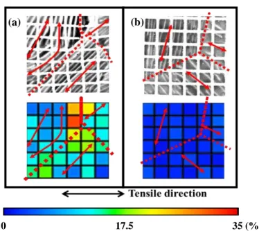
Fig. 4 indicates the distribution of strain in specimen [36] of an as-patented pearlite.

The specimen was embedded with precision markers and subjected to tensile

deformation. The lamellar alignments in both regions inclined approximately at 45

respect to the tensile direction. Even so, the distribution of strain in Fig. 4(a) is almost

the opposite of that in Fig. 4(b). Furthermore, these results are taken at a triple junction

of three colonies where strain highly concentrates [60]. Adachi et al. [66] revealed that

cementite lamellae were twisted and distorted while maintaining the crystal orientation

0 17 36 53 71 80 (%)

Fig. 3 Distribution of equivalent strain,



_eq in two adjacent colonies at nominal strain

18%

o

  . The angle between the lamellar alignment is denoted as  . The grey arrows indicate the tensile direction [62].

30 

 



 

45 18%

o

(24)

9

with the ferrite which suggests the irregularities of deformation shown in Fig. 4.

However, the two-dimension (2-D) observations of pearlite microstructure do not

provide sufficient information concerning the condition of the lamellar alignment

beyond the surface.

1.5 Complications of 2-D observations

Currently, many types of research depend on the scanning electron microscope

(SEM) [67,68] equipped with electron backscattered diffraction (EBSD) for image

analysis to acquire reliable microstructural and crystallographic data efficiently [69-74].

0 17.5 35 (%)

Fig. 4 Distribution of plastic strain pl propagation at drawing strain  5% around block/colony boundaries. (a) and (b) show three colonies with the similar lamellar

arrangement: a triple point meet. The dotted lines and arrows represent block/colony

boundaries and lamellar alignment of cementite respectfully [36].

(25)

10

Nevertheless, the existing tools and techniques only provide 2-D information from the

topography of the scanned surface. In reality, the pearlite microstructure is a complex

three-dimension (3-D) crystalline network of randomly aligned cementite lamellae

embedded in the ferrite matrixes that have various orientations. Regardless of the

arbitrary nature of the microstructure, the orientation relationships between cementite

and ferrite have been established by their interfacial planes or habit planes [75-82]. With

this knowledge, researchers assume the probable 3-D shape of the cementite lamellae

[70,71]. To understand what might be occurring inside the pearlite microstructure, the

information concerning the distribution and connectivity of cementite lamellae in 3-D

space is essential. Computer-aided reconstructions by serially sectioned images

revolutionise microstructure characterization from 2-D to 3-D visualisation [66,83-86].

However, most of the examinations is conducted with focused ion beam SEM

(FIB-SEM). The specimen is craved by the FIB gun for interval scanning. This means,

the interval sectioning eventually depletes the specimens. Hence, it physically

impossible to re-examine the 3-D morphology of the same microstructure before and

after mechanical testing [85,86]. Another option is the 3-D imaging by atom probe

topology (ATP) [87]. ATP is indeed a powerful tool that provides atomic-scale

(26)

11

observe the decomposition of cementite by counting the density of carbon atoms

[88-90]. It does not provide quantitative information such as strain mapping for

evaluating elasto-plastic deformation of microstructures. In the end, for mechanically

tested specimen, researchers are likely given no option but to rely on 2-D based

investigations.

1.6 Research outline

Chapter 1 introduces the brief history and structure of Pearlite. Pearlite colonies are

randomly aligned lamellar structures consisting of high-strength but brittle cementite

and low-strength but ductile ferrite. These microstructural features contribute to the

remarkable strength and ductility of pearlite steel. It is important to elucidate how

lamellar alignments in colonies affect the elasto-plastic deformation in colonies and

around the colony boundaries to understand the mechanical responses of colony

structures. For that purpose, 3-D observation of pearlite microstructure is necessary.

However, researchers still depend on 2-D observations. For that reason, we propose the

use of 3-D finite element analysis.

Chapter 2 explains the classical elasto-plastic theory and the established properties

(27)

12

deformation. We used commercial finite element software called ANSYS©.

In Chapter 3, we explain in details the modes of modelling 3-D colony models. The

normal vector determines the direction of lamellar alignment. From the perspective of

the normal vector, the cementite plane has two inclinations. From the orthogonal

projection, the cementite plane is inclined from the x-axis at the xy-plane. The second

inclination of the normal vector is around the axis perpendicular to the xy-plane, the

z-axis. In modelling the models, it is important to note that the angles used to describe

the lamellar alignment in each model represent the magnitude and direction of imposed

inclinations/rotations from the perspective of x-axis at xy-plane and around z-axis.

In modelling the 3D colony models, the direction of cementite lamella in 3-D space

of (x,y,z) is determined by the inclination angles of the cementite plane’s normal vector.

Two angles of inclinations describe the direction of the normal vector, the inclination

from x-axis at xy-plane and the inclination around the axis perpendicular to the xy-plane,

z-axis. The basic morphology of cementite lamella is reviewed to create the simplified

versions of 3-D single-colony finite element models. We investigated the effect of

lamellar alignment towards the elasto-plastic deformation in single-colony models.

After that, with 2-D multi-colony models, we imitated pearlite specimensto observe the

(28)

13

Chapter 4, Chapter 5 and Chapter 6 unfolds the analyses of single-colony,

multi-colonies, and double-colony conducted with 2-D and 3-D models.

In Chapter 4, a single-colony model is a multi-layered lamellar structure. This study

is the continuity of previous analyses [52,53] on pearlite lamellar structure. We studied

the mechanism behind the stability of plastic deformation in cementite phase by

layering it with ferrite. Before we can study the interaction between colonies, we need

to understand the influences which ferrite inflicts on cementite. In fine pearlite

microstructure, ferrite hardens because of size effect. To study the effect of ferrite

hardenability on the stability of cementite’s plastic deformation, we modified the

Swift’s type equation by adding a constant. Stress vs. strain relationship expresses the

mechanical response. The vertical axis and horizontal axis of the graph represents stress

and strain respectively. A constant added to the graph function for the horizontal axis

intercept. So, the constant controls the level of yield stress or level of flow stress. We

introduced possible values for the mechanical properties of ferrite by variating the

strain-hardening rate and level of flow stress. When the lamellar model subjected to

tensile deformation, the effects of ferrite’s strain-hardening rate and level of flow stress

on the stabilisation of cementite’s plastic deformation are studied. Next, we assumed

(29)

14

lamellar direction on the elasto-plastic deformations of single-colony.

In Chapter 5, we imitate the colony structures of experimental specimens into 2-D

FEM multi-colony models to compare the experimental and FEM elasto-plastic

deformation of multiple colonies.

Since the interaction between colonies is complicated, In Chapter 6, we reduces the

multi-colony models into double-colony models with 2-D and 3-D space lamellar

configuration. Reducing the models into two adjoined single-colony models connected

at the colony boundary allows us to study the fundamental interaction in colony

structure.

In Chapter 7, we discussed the results obtained by dissecting the stress components of

single-colony models to compare with stress partitioning in ferrite/cementite studies

from the crystal plasticity analyses by Yasuda and Ohashi [59]. The discussion shows

that our results agree with the plastic deformation tendencies of pearlite structure

observed experimentally by Tanaka [36]. Finally, we discuss the possible configurations

of dislocations [111-113].

The interesting aspect of this study is the approach of not considering the crystal

plasticity of cementite and ferrite. This thesis describes the understanding of the

(30)

15

Chapter 2 Analyses condition

2.1 Introduction

Tensile deformation of pearlite single- and double-colony models will be analysed by

employing the classical theory of elasto-plastic deformation in metal under uniaxial

deformation. The onset of plastic deformation in metal is defined at the limit of elastic

behaviour when the material yields the ability to return to its original form. A yield

criterion defines this condition under any combination of stresses. For the plastic

potential to be defined by such criteria constantly, certain assumptions are made. Firstly,

it is assumed that the established materials will be independent of any thermal effect.

Secondly, the materials are assumed to be isotropic. Finally, the Bauschinger effect is

neglected.

2.2 Numerical modelling of elasto-plastic deformation

(31)

16

Initially, the stress, denoted by  , is linearly proportional to strain, denoted by



along OA''. Point A is called the prop'' ortional limit. The Young’s modulus, denoted as

E, is the slope of the function.

It determines the proportionality for the increment of strain to the increment of

stress. This region is known as the elastic region. It is represented by Hooke’s law in

(1).

E

  

Fig. 5 Stress-strain curve of a typical mild steel under uniaxial tensile deformation.

(32)

17

The linear deformation is true until point A', which is called the upper yield. This

is followed by a local drop to the lower yield point, A, which is accepted as the elastic

limit. The stress value at this point is called the yield stress, denoted as Y . The stress

oscillates at a plateau to point B . The material deforms perfectly plastic through AB .

At point B , the material starts to harden. From this point, stress builds up as strain

increases until the ultimate tensile stress at point U . This is called strain-hardening,

and the material deforms plastically. If the material is unloaded at any point between

BU , for example at point C , the deformation will follow CD, which is parallel with

the initial elastic deformation path, OA. The recovered strain, DD is the elastic '

strain and denoted as el_{. Referring to (1), the elastic strain at point} _{DD is tensile}_'

stress at point C which is denoted as _c divided by the slope, which is Young's

modulus,

E

as mentioned. This gives the following equation:

el C

E

  

The remaining strain is the plastic strain, which is denoted as pl. The total strain,



t

is the sum of both regions, elastic and plastic, as shown in (2).

t el pl

pl E

 



 





 

After that, the material softens and become unstable because the stress decreases with (1a)

(33)

18

the increase of strain until it fractures at point F .

In Fig. 5, the positive slope of the true curve, which is represented by the dotted line

indicates the material is becoming stronger as it is deforming plastically. This means

that the true curve defines the strain-hardening of the material [90]. It is difficult to

determine the true stress, which is denoted as



tr, beyond the yield point. This is

because the increase of strain becomes rapid and the deformation is not uniformed

throughout the material especially after necking. On the contrary, plotting the nominal

curve is simpler because it is defined by the original parameters of the material, in

which data are measured before mechanical testing. To apply this advantage, the

nominal stress, which is denoted as _o, must be redefined by true stress.

The true stress, _tr is defined as load P divided by the instantaneous

cross-sectional area A. The representation of true stress, _tr is given by (3).

tr

P A

 

Meanwhile, true strain, which is denoted as



tr, is defined as the instantaneous length

increment, dL, per unit of the instantaneous length L . The rate of the instantaneous

strain increment is denoted as d



and is represented as:

ln dL

d L C

L







 

Hence, when the total length changes from the original length L_o , to a certain (3)

(34)

19

instantaneous length, L, it is expressed as true strain, _tr as shown in (4a).

 

ln ln ln ln

o o

L

tr L o

o L

dL L

d L L L

L L

   



   

Equation (5) shows the representation of nominal stress, which is denoted by _o. It is

defined as load, P , divided by the original cross-sectional area,

A

o.

o o P A

 

The nominal strain is denoted as _o. It is defined as the increase per unit of the original

length, L_o, as shown in equation (6).

o o o L L L   

Equation (6) can be further rearranged as:

 

1

o o

L L





And,



_o 1



o

L

L   

A plastic body is considered to be incompressible. This means the volume is

constant throughout the deformation. The changes of volume from elastic straining are

assumed to be sufficiently small and can be neglected. For that reason, the original

volume, V_o is equal to the instantaneous volume, V .

o o o

V V A L AL



(35)

20

length, L to L_o, as shown in the following (7a).

o o

A L A L

When (6a) is substituted into (7), the relationship between nominal strain, _o and the

cross-sectional areas, Ao and A are defined as follows:









1 1

o o o o

o o

A L AL

A A

 

 

Hence, the ratio of cross-sectional areas is given as:

( 1) o

o

A

A   

So, the representation of nominal stress,



_o by true stress, tr is determined in (8)

by substituting (7b) into (5).









1 1 o o o tr o P A P A         

The decrease of nominal stress, o compared with true stress,



can be

mathematically explained by substituting equation (7c) into (8).



1



o o o A A   _          

Equation (8a) proves that the instantaneous stress or true stress, _tr is unable to catch (7a)

(7b)

(7c)

(8)

(36)

21

up with the growing rate of cross-sectional area, Ao A    

  when the instantaneous

cross-sectional area,

A

of the material, rapidly decreases to compensate with the

elongation as shown in (7a). Meanwhile, the nominal strain,



o can be represented by

true strain, tr by substituting equation (6b) into equation (4a):





ln ln 1 tr o o L L     

Given that when ylnx; then xey. So, if





o1



is x and tr is y, therefore;

1 1 tr tr o o e e  



   

As shown in Fig. 5, the stress-strain curve is not straight forward. To model the

stress-strain relationship of a material subjected to tensile deformation, idealisation for

elasto-plastic deformation needs to be considered. For this case, two types of

elasto-plastic idealisation shown in Fig. 6 are employed. Fig. 6(a) is elastic-perfect

plastic material. It will be applied to establish brittle material. Fig. 6(b) is power plastic

hardening material. It will be applied to establish ductile material. The non-linear work

hardening will be represented by empirical equations type Swift [92]. These will be

further elaborated in the next section.

(9)

(37)

22

2.3 Material properties

Fig. 7 shows the stress-strain curves established for cementite and ferrite in this study.

We used Poisson’s ratio 0.3 for both materials. Young’s modulus of bulk cementite

ranges from 176 GPa to 186 GPa [42]. At room temperature, cementite fractures at its

yield point, 2.75 GPa [42,43,89]. The Young’s modulus, E , for cementite is the

arithmetic mean of its Young’s modulus, which is E181GPa. When the yield stress

for cementite is denoted as Y, then, from the Hooke’s law, the elastic limit for

cementite at nominal strain, _o is calculated in (10):

2

2.75

1.593 10 181

o

Y GPa

E GPa



 _ _ _ _ 

Fig. 6 Idealisation of elasto-plastic deformation. (a) Elastic-perfect plastic material, and

(38)

23

Interestingly, Kanie et al. [94] experimentally proved the cementite can bear elastic

strains, el around 1% to 2%. However, it is tricky to simulate the brittle property of

cementite numerically. Theoretically [95-97], the condition of plastic instability occurs

prior to the onset of necking at the maximum load point. Load P is always

proportional to the product of true stress, tr multiplied by the cross-sectional areaA.

So, the condition for maximum load point is given in (11).

0 tr

tr tr

P A

dP Ad dA



 



  

During the plastic deformation, the volume of material is considered to be constant, as

shown in (7). To fit (7) into the condition for maximum load point, it is differentiated on Fig. 7 Stress-strain curves for cementite and ferrite

Tru

e

stre

ss

tr 

(M

Pa)

True plastic strain



trpl

(%)

Cementite

Ferrite

(39)

24

the instantaneous area, A to obtain dA in (12):

0

o o

AL A L AdL LdA dL dA A L     

When (4a) is substituted into (12) the relationship between area and strain is derived.

tr

dA Ad



  

The strain-hardening rate is obtained by substituting (12a) into the condition of

maximum load point, dP0 from (11).

0

tr tr tr tr tr tr Ad Ad d d     _    

For our analyses, cementite is modelled after the elastic-perfect plastic model. The

strain-hardening rate for cementite is 0 because it is constant. The cross-section A

rapidly becomes smaller to maintain the material's volume, V at yield stress. Meaning,

cementite undergoes necking at the moment it yields. This condition is highly unstable

because cementite is unable to harden..

The stress-strain curve for ferrite is modelled by power plastic hardening material

idealisation. It is represented by the following Swift’s type equation [92]:



_pl



N tr a b

  

This equation is a generalised power law, where true stress, _tr is an exponential product of plastic strain, pl. Here, a , b and N are empirical constants determined (12)

(12a)

(12b)

(40)

25

experimentally by Umemoto [99]. Their values are a493 MPa, b0.002 and

0.28

N respectively.

strain,



t relationship. Since the plastic flow is determined by Swift’s type equation

mentioned above in (13), the values for each true stress,



_tr can be determined by any

given plastic strain,



pl . The elastic region is determined by Hooke’s law as

aforementioned in the earlier section. Therefore, the total strain,



t is

t tr pl

E





 



For our analyses, the data input for cementite and ferrite follows the true curve. On the

contrary, the models are given forced displacements, so the analysis results or

simulation data are plotted nominally. Fig. 8 shows the difference between the true and

nominal curve for cementite. The stress values for simulation data, which are

represented by the nominal curve, will decrease around yield point because the

instantaneous cross-section area A, was neglected to simplify the data harvesting.

2.4 von Mises yield condition

The onset of plastic deformation in metal occurs when the combination of stresses in

(41)

26

expressed in (15) defines the critical value.

2 2

J k

The second deviatoric stress, commonly written as J₂ is related to the changes of the

material shape. The yield stress in simple shear is given as k . Since there are six

components of stress, J₂, (15) can be represented as follows:

2 2 2 2 2 2

2 ( xx yy) ( yy zz) ( zz xx) 6 xy 6 yz 6 zx

J               

When a material is under multiaxial loading condition, the equivalent stress denoted as

eq



is defined in (16).

2

3

eq J

 

Fig. 8 Stress-strain curve for true and nominal curve for cementite. This figure shows

the plastic flow stress for elastic-perfect plastic material stress established for cementite in comparison to the simulated data.

(15)

(15a)

(42)

27

Square both sides of the (16) and then substitute (15a) into the equation.







 





 







2 2

2 2 2 2 2 2

2 2 2

3

3 ( ) ( ) ( ) 6 6 6

3 ( ) ( ) ( ) 3 6 6 6

3

( ) ( ) ( ) 3

6 1

( ) ( ) ( )

2 eq

xx yy yy zz zz xx xy yz zx

xx yy yy zz zz xx

J                                                              

      ₃



2 2 2



xy yz zx

  

Multiply both sides of (16a) with 2 to even the denominator of the equation.

2 2 2 2 2 2 2

2_eq(_xx_yy) (_yy_zz) (_zz_xx) 6_xy6_yz6_zx

Thus, the equivalent stress,



_eq is expressed as (15c).

2 2 2 2 2 2

( ) ( ) ( ) 6 6 6

2

xx yy yy zz zz xx xy yz zx

eq

        

         

This form is also known as the von Mises stress. From (15), the relationship in (16a)

can also be expressed as (17).

2 2

2

3 3

eq J k

  

In the case of uniaxial stress, the yield stress in simple shear relationship with the tensile

yield stress, Y, is given in (18).

3

Y k

Square both sides of (18).

(43)

28

Compare (17) and (18a).

2 2 2

3

eq k Y

  

From (18b), if _eq2 Y2, therefore (16b) can be rearranged into (18c).

2 2 2 2 2 2 2

(_xx_yy) (_yy_zz) (_zz_xx) 6_xy6_yz 6_zx2Y

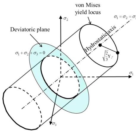
This equation defines the yield surface of the von Mises circular cylinder in the

principal stresses space, which is denoted by ₁, ₂, and ₃, as shown in Fig. 9. The

von Mises yield locus is 2

3Y.

In equation (18), the von Mises yield condition proposed that the onset of plastic

deformation is when the equivalent stress or the von Mises stress,



_eq is equal to the

tensile yield stress, Y . By neglecting the Bauschinger effect, any stress points on the

surface of the cylinder will correspond to a state of yielding. Whereas, any stress points

inside the cylinder correspond to a state of elastic deformation. In simple tension, (18b)

can be further simplified as (19).

(44)

29

In Fig. 9, the cylinder is inclined so that the direction cosines of the hydrostatic axis

of each of the principal stress axes are equal, (1 / 3,1 / 3,1 / 3). Thus, at the

hydrostatic axis, the principal stresses are equal,  ₁ ₂₃. On the other hand, the

deviatoric plane where the sum of principle stresses are equal to zero,   ₁ ₂ ₃0,

is perpendicular to the hydrostatic axis. These configurations imply that the von Mises

yield locus is not only parallel to the deviatoric plane, but also symmetrical at the



1-,

2



-,



3and -axes. The uniform hydrostatic stress does not affect the yield state of a

Fig. 9 Diagram of the von Mises yield condition in the principal stress space.

(45)

30

deforming body. The hydrostatic stress influences volume change, therefore, the volume

of the material is constant after yielding. von Mises yield condition depends on the

magnitude and direction of the deviatoric stress, as defined in (15).

2.5 The associative flow-rule

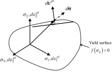
The associated flow-rule [101,102] is defined when the plastic potential of the

material is the yield function. In other words, the flow rule is associated with a

particular yield condition. In this study, von Mises yield condition is employed. Fig. 10

shows the axes of principal stress and principal plastic strain, which are denoted as

1, 1 pl

d

  ,  ₂,d ₂pl and  ₃,d ₃pl; and their relationship with the plastic strain increment

vector, which is denoted as dεpl

.

The vector of principal stress, is denoted as dσ. The

normal to the yield surface is given as the differentiation of yield function f

 

_ij

(46)

31

towards the vector of the principal stress dσ.



_ij is the multiaxial stresses. This is

called the normality rule and it has been confirmed experimentally on metals. The

equation of the associate flow-rule is given as:

pl ij

ij f

d d

  



f is the yield function and d is the principal deviatoric stresses and principal plastic

strain increments. In 3-D space, which axes constitute of (x, y, z); the ( d) is expressed

by (20a), where the stress deviations are denoted as sxx,s ,yy szz,s ,xy s ,yz szx.

pl pl pl

yy xy yz

xx zz zx

xx yy zz xy yz zx

d d d

d

s s s s s s

  

 _ _  _ _ _  _ _

The stress deviations represented by s are the subtracts of mean normal stress which _ij

is denoted as s from the normal stress tensors which are represented by



_ij.

ij ij

s  s

The mean normal stress relationship with normal stress is defined in (22).





1

3 xx yy zz

s   

By applying the von Mises yield condition in (19) to the example of tensile deformation

in the direction of x, the non-vanishing stress component is



xx. The non-vanishing

stress component for y and z direction are shown in (22b) together with x.

(47)

32

Regarding normal stresses, the stress-plastic strain relationships are given as:













2 1 3 2 2 1 3 2 2 1 3 2 pl

xx xx yy zz

pl

yy yy xx zz

pl

zz zz xx yy

pl xy xy pl yz yz pl zx zx d d d d d d d d d d d d                         _   _      _   _      _   _     

Prandtl-Reuss equations [102-104], and the equations are represented using Hooke’s

law as follows:

























1 2 1

3 2

1 2 1

3 2

1 2 1

3 2

1

1 pl

xx xx yy zz xx yy zz

pl

yy yy xx zz yy xx zz

pl

zz zz xx yy zz xx yy

pl

xy xy xy

pl

yz yz yz

d d d d d

E

d d d d d

E

d d d d d

E

d d d

E

d d d

E d                                          _   _ _   _        _   _ _   _        _   _ _   _         1 pl

zx d zx d zx

E  



 

(23)

(48)

33

Chapter 3 Modelling of pearlite colony

3.1 Morphology of cementite in pearlite

The morphology and evolution of pearlite microstructure is a subject of interest.

Researchers are intrigued by the plastic deformability of cementite inside of pearlite

because it determines the plastic deformation of pearlite [22]. The revision of literature

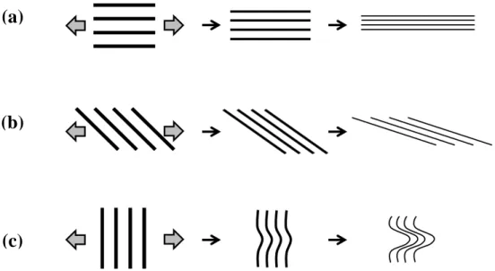
reviews [22,37,40,41,63] disclosed that many studies agreed on categorising the

morphology of cementite in pearlite during tensile deformation into three main types as

shown in Fig. 11. In Fig. 11(a), the alignment of cementite is parallel to the tensile axis.

In Fig. 11(b), the alignment of cementite is inclined at a certain degree of inclination

angle, from the tensile axis. In Fig. 11(c), the alignment of cementite is perpendicular to

the tensile axis. From the tensile axis point of view, if the lamellar alignment is parallel

to the tensile axis, the angle is 0, whereas, if the lamellar alignment is perpendicular

to the axis, the angle is 90. Therefore, the range for the inclination angle of a colony

(49)

34 45

 , the lamellar structure suffers maximum shear stress [44,56,57,99]. Therefore,

this angle will be considered for the model type illustrated in Fig. 11(b).

3.2 Defining the alignment of cementite lamella in 3-D space

In calculating, the inclination angle of lamellar alignment in pearlite, Belaiew [32]

assumed that cementite and ferrite lamellae are parallel and are closely packed inside a

sphere. Inside a sphere, the coordinate of a point is determined by two angles from the

orthogonal plane and the axis perpendicular to the orthogonal plane. Therefore the

position of the lamella alignment in a 3-D space is explained using the idea of spherical

coordinates.

(b)

(a)

(c)

(50)

35

(a)

(b)

Fig. 12 Schematic of 2-D orthogonal projection and 3-D view of a pearlite colony. (a) is the

orthogonal projection of cementite ( ) and ferrite () lamellar. (b) The direction of the  plane is determined by the direction of normal vector, n. The direction of n is determined by the azimuthal angle at the xy-plane,



and the inclination angle

トップページ 北見工業大学学術機関リポジトリ（KITR） LIDYANA 学位論文

El as t o- pl as t i c def or m

at i on anal ys es of t he

i nt er ac t i on of c ol ony s t r uc t ur es i n t he

m

i c r os t r uc t ur e of pear l i t e s t eel s

その他のタイトル

（パーライト鋼の微視組織におけるコロニー間の相

互作用に関する弾塑性変形解析）

著者

LI D

YAN

A BI N

TI RO

SLAN

学位名

博士（工学）

学位授与機関

北見工業大学

学位授与番号

10106甲第156号

研究科・専攻名

生産基盤工学専攻

学位授与年月日

2017- 03- 17

博

士

論

文

Doctoral Thesis

Elasto-plastic deformation analyses of the interaction of

colony structures in the microstructure of pearlite steels

2017

3

2017

March

要旨

ABSTRACT

Contents

List of figures







List of table

Chapter 1

Overview

1.1

Introduction

1.2

Pearlite microstructure

1.3

Deformation of cementite in pearlite

1.4

Deformation of block/colony structures in pearlite



30



 



 

45

18%

1.5

Complications of 2-D observations

1.6

Research outline

Chapter 2

Analyses condition

2.1

Introduction

2.2

Numerical modelling of elasto-plastic deformation



E



 



 





トップページ北見工業大学学術機関リポジトリ（KITR） LIDYANA 学位論文