Development of an Unstructured Grid Solver for Complex Wave Impact Problems
モハメド ムスタファ ザキ アハメド カムラ
http://hdl.handle.net/2324/1959162
出版情報:九州大学, 2018, 博士(学術), 課程博士 バージョン:
Development of an Unstructured Grid Solver for Complex Wave Impact Problems
by
Mohamed Moustafa Zaki Ahmed Kamra
Submitted to the Earth System Science and Technology in partial fulfillment of the requirements for the degree of
Doctor of Philosophy in Engineering
at
Kyushu University
September 2018
c Kyushu University 2018. All rights reserved.
Development of an Unstructured Grid Solver for Complex Wave Impact Problems
by
Mohamed Moustafa Zaki Ahmed Kamra
Submitted to the Earth System Science and Technology on September 25, 2018, in partial fulfillment of the
requirements for the degree of Doctor of Philosophy in Engineering
Abstract
During the past two decades, much attention has been directed to the development of accurate simulation tools for wave impact problems. The significance of the research can be found in the maritime industry, ocean engineering, and coastal engineering. In the offshore industry, offshore structures must survive severe weather conditions includ- ing very large waves for many years and sometimes decades. For coastal engineering, wave impact problems are also important for the protection of coastal structures and stopping the recession of coastal lines. This requires accurate prediction of impact load- ing on coastal structures by very large waves such as tsunami waves. Therefore, there is a great need for development of accurate simulation methods which are capable of predicting those impact loads and providing better understanding of wave impact phe- nomena. A promising method is the computational fluid dynamics (CFD) method based on the solution of Navier-Stokes equations of multi-fluid turbulent flow.
The objective of this research is to develop an efficient CFD solver for accurate prediction of violent free surface motion and wave impact loading on structures with complicated geometry. To achieve that goal, a CFD solver that is based on the Navier- Stokes equations which describe the motion of the incompressible turbulent flow on unstructured meshes has been developed. The finite volume approach is employed to discretize the governing equations. The free surface is treated by the volume of fluid (VOF) method. The promising and attractive unstructured multi-dimensional tangent hyperbolic interface capturing method (UMTHINC) is used for interface capturing. The method combines the accuracy of geometric reconstruction VOF methods with the sim- plicity of algebraic based methods which allows for easy and efficient implementation on unstructured meshes.
iii
impact phenomena. The dam break impact against a vertical cylinder is chosen as a model problem for this investigation. The main results of this work are as follows:
Error analysis is conducted to study the influence of parameters on the accuracy and stability of the UMTHINC method. The boundedness of the method is found to be compromised at high Courant numbers and sharp interfaces (i.e. the interface is diffused over few cells). The cause of this problem has been identified and a solution that ensures that the VOF field remains bounded without any mass loss has been proposed. The accuracy of the revised method is evaluated using several benchmark cases and it shows competitive accuracy with existing numerical results of other methods in literature.
A new experiment of dam-break impact flow against a vertical wall and a vertical cylinder with square or circular cross-section has been conducted. The aim of the ex- periment is to provide high resolution free surface images and more reliable pressure measurements than those in literature. A novel gate motion profile, obtained from the best fits of the gate motion measurements, has been proposed. A direct correlation is found between the parameters of the proposed motion profile and the wave impact event.
Utilizing the newly obtained experimental data, the accuracy of the developed fluid solver has been confirmed both kinematically and dynamically. A novel simplified model for the gate motion in the dam-break experiment is developed and implemented on unstructured grids. The effect of the gate motion on the wave-front speed is clearly demonstrated. The effect of the cylinder cross-section on the impact loading and on the free surface variation is studied. The square cross-section is found to produce flow a field with higher turbulence which is clearly depicted in the free-surface profiles and pressure loading histories. The impact with the circular cross-section is found to be rather mild in comparison with the square cylinder while the impact phenomenon on the vertical wall is more violent. This is owing to the different nature of flow separation for different cross-section of the cylinder.
Finally, an investigation of the effect of the turbulence model on the flow character- istics, separation patterns, and impact loading on the obstacle and vertical wall has been conducted and discussed. The RANS models are found to predict very similar results prior to the impact and the difference between the models is observed after the impact.
The LES model is found to require a much finer mesh in order to provide accurate predictions, otherwise the predicted solution would contain excessive diffusion. This shows that a proper choice of turbulence model has a very important effect in obtaining accurate predictions for separated flows and thus requires further investigation.
Thesis Supervisor: Dr. Changhong Hu Title: Professor
Date: 25/9/2018
Acknowledgments
First and foremost I wish to express my deepest gratitude and sincere thanks to my supervisorProfessor Changhong Hufor his instructive supervision, continuous guid- ance, valuable instructions and offering of all facilities. You have devoted your intellec- tual energies and high sense of profession in the supervision of this thesis. Without your creative thinking, valuable suggestions and constructive criticism, the fulfillment of this work would have been extremely difficult. I am thankful for your caring and concern, and faith in me throughout this projected journey. I have learned a great deal and gained valuable experience.
I must thank the Japanese government for the Ministry of Education, Culture, Sports, Science, and Technology (MEXT) scholarship which funded my PhD project. I also thank the Interdisciplinary Graduate School of Engineering Sciences(IGSES)for fund- ing my conferences and internship expenses.
Kyushu Universitycommunity has provided a stimulating environment for learning and growing. I learned a lot through the interactions with the faculty members, post- doctoral fellows, and graduate students. I would also like to thank all theEarth System Science and Technology (ESST)Department administrative members for their prompt and professional assistance whenever I needed specially Dr. Makoto Sueyoshi, Dr.
Cheng LIUandMs. Masako Yoshizu.
A special thank you goes to my friends Amr Halawa, Amr Metwally, Moustafa RushdiandDr. Tarek Dief. I will never forget our gathering; you are wonderful guys and true friends. Thank you so many guys for a great time together; my life at Fukuoka was made enjoyable mainly due to you.
A special thank you goes to my professors in Cairo University for their support, help, and guidance which they gave me during my bachelor and master specially Professor Atef SherifandDr. Basman El Hadidi.
Whatever I say or write, I will never be able to express my deep feelings and pro- v
of science, you have always believed in me, and you have never stopped to support and encourage me. Thank you for your patience throughout all the years. I am forever grateful.
I would also like to express my deepest gratitude to my beloved wife and sonfor their consistent love and support during the past three years which was a great driving force for me.
Thanks
Mohamed M. Kamra Kyushu University September, 2018
Declaration
No portion of the work referred to in the thesis has been submitted in support of an application for another degree or qualification of this or any other university or other institute of learning.
vii
Contents
1 Introduction 1
1.1 Background and Motivation . . . 1
1.2 Review on Turbulence Modeling . . . 3
1.3 Review of Interface Capturing Methods . . . 4
1.4 Dam-break Flow . . . 7
1.5 Thesis Objective and Outline . . . 10
2 Mathematical Model 13 2.1 Navier-Stokes Equations . . . 14
2.2 Two-Fluid Flow Modeling . . . 14
2.3 Modeling of Surface Tension Force . . . 15
2.4 Turbulence Modeling. . . 16
2.4.1 Standardk−εModel . . . 16
2.4.2 Realizablek−εModel . . . 17
2.4.3 Wilcoxk−ω Model . . . 18
2.4.4 Smagorinsky Sub-Grid Scale Model . . . 19
2.5 Initial and Boundary Conditions . . . 20
2.5.1 Initial Conditions . . . 20
2.5.2 Boundary Conditions . . . 21
2.6 Closure . . . 23 ix
3.1 Computation of Gradient . . . 26
3.1.1 Green-Gauss Gradient . . . 26
3.1.2 Least Square Gradient . . . 30
3.2 Volume Fraction Equation . . . 31
3.3 The Momentum Equation . . . 33
3.3.1 The Convection Term . . . 33
3.3.2 The Time Derivative Term . . . 34
3.3.3 The Diffusion Term . . . 35
3.4 Pressure-Velocity Coupling . . . 37
3.5 Turbulence . . . 40
3.6 Boundary Conditions . . . 42
3.6.1 Inlet Boundary . . . 42
3.6.2 Open Boundary . . . 44
3.6.3 Rigid Wall Boundary . . . 45
3.6.4 Shell Boundary . . . 47
3.6.5 Symmetric-Plane Boundary . . . 48
3.7 Solution Procedure . . . 49
3.8 Closure . . . 49
4 UMTHINC Method 51 4.1 Basic Description . . . 52
4.2 Computation of the Interface Normal . . . 54
4.3 Computation of the Parameter (d)e . . . 57
4.3.1 Hexahedral Cell . . . 57
4.3.2 Tetrahedral Cell. . . 60
4.3.3 Prism Cell . . . 61
4.3.4 Pyramid Cell . . . 64
4.3.5 Evaluation of the Accuracy of the Parameterde . . . 65
4.4 Computation of the Volume Fraction Face Value (αf) . . . 70
4.5 Stability Issues With UMTHINC . . . 71
4.6 Test Cases . . . 77
4.6.1 Boundedness Error of the Volume Fraction . . . 79
4.6.2 Interface Reconstruction of a Circle . . . 83
4.6.3 Standard Benchmark Cases. . . 85
4.7 Closure . . . 91
5 Dam Break Experiment 93 5.1 Experiment Setup. . . 94
5.1.1 Tank and Gate Release System . . . 94
5.1.2 Data Acquisition System . . . 94
5.1.3 Experiment Operating Conditions . . . 97
5.1.4 Sources of Uncertainty in the Experiment . . . 98
5.2 Experiment Results . . . 101
5.2.1 Gate Motion Repeatability Analysis . . . 101
5.2.2 Obstacle Impact Time . . . 103
5.2.3 Pressure Measurement . . . 106
5.2.4 Free Surface Profile . . . 109
5.3 Closure . . . 112
6 Validation Cases: Dam Break Flow 113 6.1 Solver Configuration . . . 113
6.2 Dam Break Against a Vertical Wall . . . 116
6.3 Dam Break Against a Vertical Cylinder . . . 132
6.4 Closure . . . 145 xi
7.1 Summary . . . 147 7.2 Future Research . . . 149
References 151
List of Figures
1-1 Offshore wind turbines. NREL,2018 . . . 2
1-2 Wave impact on coastal structures (source: http://www.panoramio.com/photo/48851473) . . . 2
1-3 DNS (left), LES (middle) and RANS (right) simulation of a turbulent jet. Image Source: New Developments in the Visualization and Pro- cessing of Tensor Fields[44] . . . 3 2-1 Schematic drawing of wall adhesion and wetting angle(θeq) . . . 22 2-2 Drawing of the shell boundary condition . . . 23 3-1 Computational stencil of the Cell-based Green-Gauss gradient(Compact
Stencil) . . . 27 3-2 Computational stencil of the Node-based Green-Gauss gradient(Extended
Stencil) . . . 28 3-3 Drawing of a decomposed three-dimensional face in the Node-based
Green-Gauss gradient method . . . 29 3-4 Computational stencil of the Least-Square gradient (green: Compact
Stencil, red: Extended Stencil) . . . 31 3-5 Determination of upstream and downstream cells depending on flow
direction . . . 34 3-6 Flow chart of the implemented PISO procedure . . . 41
xiii
3-8 Relation between and in the turbulent boundary layer . . . 47
3-9 Discrete shell boundary condition . . . 48
3-10 Flow chart of the solution algorithm . . . 50
4-1 One dimensional approximation of the THINC method . . . 53
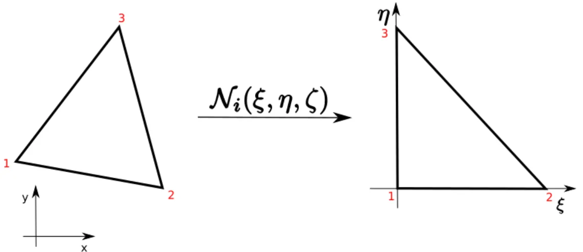
4-2 Cell transformation to reference cell shape using basis functionsN (ξ,η,ζ) 55 4-3 Canonical Hexahedral cell . . . 58
4-4 Canonical Tetrahedral cell . . . 60
4-5 Canonical Prism cell . . . 62
4-6 Canonical Pyramid cell . . . 64
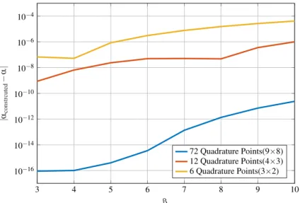
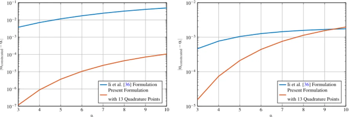
4-7 Comparison of accuracy of the parameterdefor a hexahedral cell where α =0.01 (left) andα=0.50 (right), with(mξ =mη)>mζ . . . 66
4-8 Comparison of accuracy of the parameterdefor a hexahedral cell where α =0.01(left) andα =0.50(right), andmξ >mη >mζ . . . 67
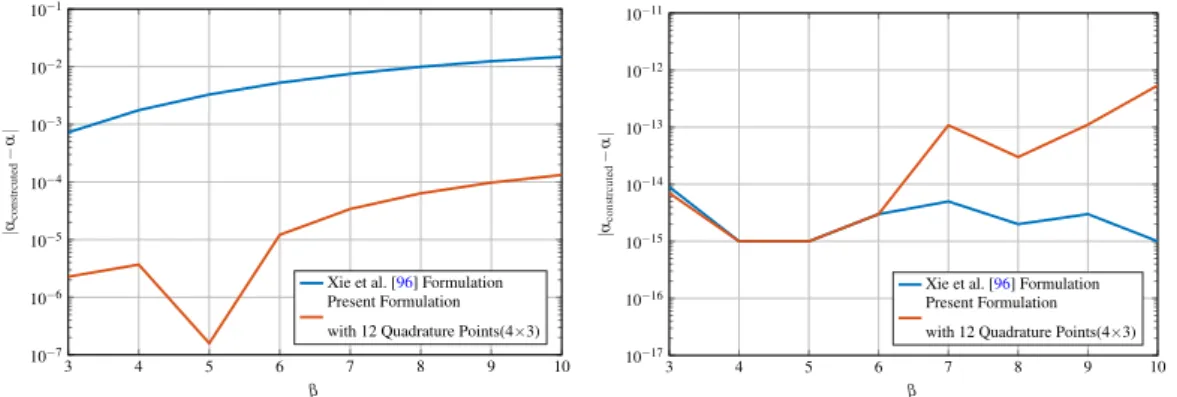
4-9 Comparison of accuracy of the parameterdefor a hexahedral cell where α =0.01, andmξ >mη >mζ with different number of Quadrature points 67 4-10 Comparison of accuracy of the parameterdefor a tetrahedral cell where α =0.01(left) andα =0.50(right), and(mξ =mη)>mζ . . . 68
4-11 Comparison of accuracy of the parameterdefor a tetrahedral cell where α =0.01(left) andα =0.50(right), andmξ >mη >mζ . . . 69
4-12 Comparison of accuracy of the parameterdefor a tetrahedral cell where α =0.01, andmξ >mη >mζ with different number of Quadrature points 69 4-13 Overlap of the transport areas for the volume fraction . . . 72
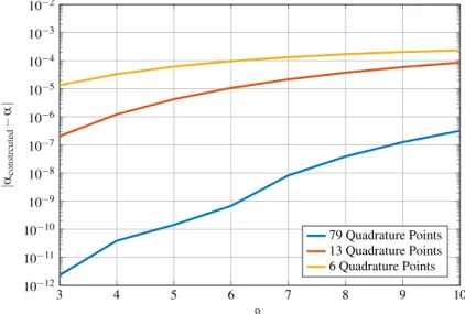
4-14 Flux polygon construction of the EMFPA[31, 55] approach and Jofre et al. [39] approach . . . 73
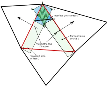
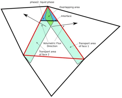
4-15 Overlap of the transport areas for the volume fraction in the UMTHINC method . . . 75
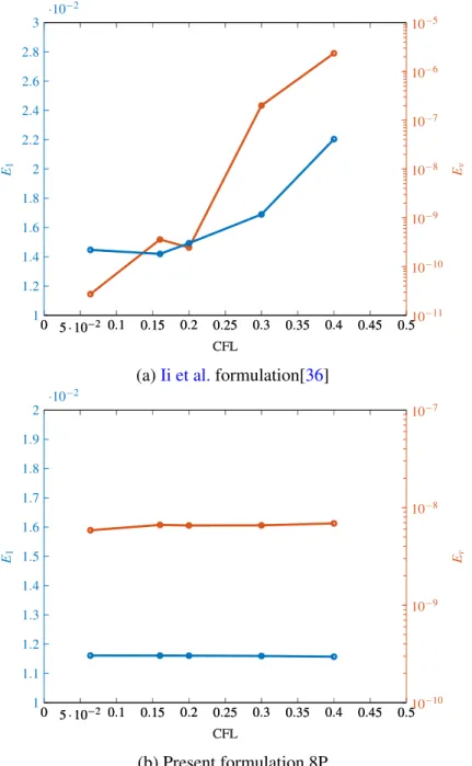
4-16 The computational grids used in test cases . . . 78 4-17 Maximum over/undershoots at t = π2 withCFL=0.10. . . 80 4-18 Maximum over/undershoots at t = π2 withCFL=0.40. . . 81 4-19 Numerical errorE1and volume change errorEv atβ =4 with different
CFL numbers in comparison with Ii et al. formulation[36] . . . 82 4-20 Numerical errorE1with differentβ values atCFL=0.1 and 0.4 differ-
ent number of quadrature points . . . 83 4-21 Error of interface reconstruction of a circle using different methods to
obtain the interface normal on triangular mesh with different resolutions 84 4-22 Enlarged view of the interface (0.5-contour) after one revolution for Za-
lesak’s slotted disk. The red line is numerical result and the black is the exact solution . . . 86 4-23 Enlarged view of the interface (0.5-contour) after one revolution for
Rudman’s slotted disk. The red line is numerical result and the black is the exact solution . . . 87 4-24 Numerical results of the 2D shearing vortex flow for T = 8. The blue
line is the numerical result att =T/2 , the red line is att =T and the black is the exact solution . . . 90 5-1 Schematic drawing of the problem of dam-break against a vertical cylin-
der(top left ,and top right respectively), and sensor placement on the cylindrical obstacle(bottom left) and the right vertical wall( bottom right ) (all dimensions are in mm) . . . 95 5-2 Schematic drawing of the gate release system . . . 96 5-3 Overall setup of the dam break experiment . . . 97 5-4 Zoom on the leading of the installed pressure on the circular cylinder . . 99 5-5 Rigid body analysis of the gate release motion . . . 99 5-6 Analysis of gate motion for all experiment trials . . . 102
xv
pressure sensor . . . 104
5-8 Cumulative probability function for the wave impact time with the ob- stacle . . . 104
5-9 Correlation of gate motion to obstacle impact time. . . 105
5-10 Cumulative probability function for the duration between the impact with the cylinder and the impact with the vertical wall . . . 106
5-11 Pressure measurement on the cylindrical obstacle . . . 107
5-12 Pressure measurement on the vertical wall . . . 107
5-13 Free surface evolution for square cylinder . . . 109
5-14 Free surface evolution for circular cylinder . . . 110
5-15 Free surface time evolution for the no obstacle case . . . 111
6-1 Illustration of the developed gate model for dam-break flow simulations 115 6-2 Schematic of dam-break simulation against a vertical wall . . . 116
6-3 Mesh independence test . . . 117
6-4 Computational mesh for the dam-break flow against vertical wall . . . . 118
6-5 Wave front propagation at H = 0.2m, compare to literature . . . 119
6-6 Comparison of the free surface profile(3D Iso-metric view) at selected time instances . . . 122
6-7 Pressure measurement on the vertical wall . . . 123
6-8 Comparison of the free surface profile(front view) at selected time in- stances. The left: 2D section at the domain center line(red:3D, blue:2D), middle: 3D perspective front view, right: experiment perspective front view . . . 125
6-9 Velocity vectors in the bottom right corner area of the impacted wall (taken at the x-y plane) at the moment of impact. The figure is a mag- nified bottom view of the corner where the blue region represents water and the white represents air . . . 126 6-10 Schematic drawing of the problem of dam-break against a vertical wall(left),
and sensor placement on the right vertical wall(right) (all dimensions are in cm) . . . 127 6-11 Time history of the pressure at the vertical wall . . . 128 6-12 Pressure distribution in the transverse direction at the vertical wall . . . 129 6-13 Effect of tank width on the pressure distribution in the transverse di-
rection at the vertical wall with left ( W = 0.1m) and right (W = 0.3m) . . . 131 6-14 Schematic of dam-break simulation against a vertical cylinder . . . 132 6-15 Computational mesh for the dam-break flow against a circular vertical
cylinder . . . 133 6-16 Computational mesh for the dam-break flow against a square vertical
cylinder . . . 134 6-17 Comparison of the free surface profile at selected time instances be-
tween the numerical solution (left), and experiment (right) for the cir- cular obstacle case . . . 137 6-18 Comparison of the free surface profile at selected time instances be-
tween the numerical solution (left), and experiment (right) for the square obstacle case . . . 139 6-19 Comparison of the free surface separation pattern, behind the vertical
cylinder, between the circular (left) and square(right) cross-sections . . 140 6-20 Pressure measurement on the cylinder at(0.575, 0.1, 0.011) . . . 141 6-21 Pressure measurement on the vertical wall at(0.8, 0.1, 0.004) . . . 141
xvii
downstream vertical wall for the two considered cross-sections . . . 142 6-23 Comparison of the computed pressure force on the circular cylindrical
obstacle and the downstream vertical wall for different turbulence mod- els . . . 143 6-24 Comparison of the computed pressure force on the circular cylindrical
obstacle and the downstream vertical wall for different turbulence mod- els . . . 143 6-25 Magnified view of the sub-grid eddy viscosity at the impact wall. Sec-
tion taken aty=0.1. . . 144
List of Tables
3.1 Listing of the TVD limiter functions employed in this work . . . 34
4.1 Numerical errors of Zalesak’s rotation problem on quadrilateral meshes in comparison with the published numerical results of UMTHINC and THINC/QQ[97] . . . 86
4.2 Numerical errors of Zalesak’s rotation problem on triangular meshes in comparison with the published numerical results of UMTHINC and THINC/QQ[97] . . . 86
4.3 Numerical errors of Rudesak’s rotation problem on quadrilateral meshes in comparison with the published numerical results of UMTHINC and THINC/QQ[97] . . . 88
4.4 Numerical errors and convergence rates of the 2D shearing problem in comparison with the reported numerical results of other VOF schemes[30, 55, 73] and THINC/QQ[97] . . . 90
5.1 Physical properties at temperature of 10◦C . . . 98
5.2 Number of trial runs conducted for each experiment . . . 101
6.1 Solver configuration parameters . . . 114 6.2 Mesh spacings of the three grid adopted in the mesh independence test . 117
xix
t∗>1 . . . 119 6.4 Coefficients of the fitted equations for numerical and experimental data
of the time history of the wave front position as in Figure 6-5 . . . 120 6.5 The non-dimensional average velocityv/√
ghof the wave front toe for t∗>1 . . . 123
Chapter 1 Introduction
Contents
1.1 Background and Motivation . . . 1 1.2 Review on Turbulence Modeling . . . 3 1.3 Review of Interface Capturing Methods . . . 4 1.4 Dam-break Flow . . . 7 1.5 Thesis Objective and Outline . . . 10
1.1 Background and Motivation
During the past two decades, much attention has been directed to the development of accurate simulation tools for wave impact problems. The significance of this can found in maritime industry, ocean engineering, and coastal engineering. In the offshore in- dustry, structures are placed in oil or gas fields for many years and sometimes decades.
These structures must survive different weather conditions including high and vio- lent waves. In such conditions, offshore structures face the problem of wave impact on
1
Figure 1-1: Offshore wind turbines. NREL,2018
Figure 1-2: Wave impact on coastal structures
(source: http://www.panoramio.com/photo/48851473)
their bow or bottom. Furthermore, in high wave conditions, water can flood the deck level of the structure causing damages to equipment on deck [25, 61]. This is known as green water and it is an important problem not only to offshore structures but also to large ships at sea [11]. In addition to offshore and ocean engineering, wave impact prob- lems are also important for the protection of coastal structures and stoping the recession of coastal lines. This warrant accurate prediction of impact loading on coastal structures from violent waves or in the extreme case of tsunami impact. Thus, there is a great need for the development of accurate simulation tools capable of prediction of impact loads resulting from green water or violent waves and provide a better understanding of im- pact phenomena. A good prediction is based on the solution of Navier-Stokes equations of turbulent incompressible two-fluid flow.
3 1.2. REVIEW ON TURBULENCE MODELING
1.2 Review on Turbulence Modeling
Turbulence is often modeled using one of the following methods; Direct numerical sim- ulation (DNS), Reynolds averaged-Navier Stokes (RANS) equations, and Large Eddy Simulation (LES).
DNS [64] refers to simulations where the Navier-Stokes equations are numerically solved without any turbulence model. This means resolving the whole spectrum of spatial and temporal scales of the turbulence. All the spatial scales of the turbulence must be resolved in the computational mesh, from the smallest dissipative scales (Kol- mogorov scale), up to the largest length scales, associated with the motions. In addition to the substantially dense computational mesh, discretization is usually conducted us- ing high-order spatial and temporal schemes further increasing the computational cost.
Theoretically, DNS can be used to solve any turbulent flow but due to it sever computa- tional requirements its application has been limited to low Reynolds numbers flows in small scales. This would make it inapplicable to engineering applications.
Figure 1-3: DNS (left), LES (middle) and RANS (right) simulation of a turbulent jet. Image Source: New Developments in the Visualization and Processing of Tensor Fields[44]
CHAPTER 1. INTRODUCTION
Alternatively, several turbulence models were developed to capture turbulent flows while maintaining a reasonable computational cost. RANS models are very popular and widely accepted choices in that department. In RANS models, only time-averaged (mean) field are described and turbulence effects are introduced to the momentum equa- tions using Reynolds stress. The Reynolds stresses are modeled using the Boussinesq approximation and the turbulent/eddy viscosity is computed using a suitable RANS model. RANS models such as thek−ε andk−ω models were successfully used in the predictions of wave impact dynamics [8,42,50,67,99, 100]. In this study, the fol- lowing RANS models are considered: the standardk−ε, realizable k−ε, and Wilcox k−ω models.
Another alternative is LES model, which directly solves the large three-dimensional unsteady turbulent motions and models the sub-grid scales. From a computational ex- pense point of view, LES lies between DNS and RANS because it solves large scales directly thus it is expected to be more accurate than RANS and it models the smallest scales so it reduces the computational cost when compared to DNS. LES models were also widely used in wave impact cases[5,45,50] however due to its demanding compu- tational cost, many scholars prefer using RANS models. In this study, the Smagorinsky LES is presented to provide a comparative factor with the RANS models.
1.3 Review of Interface Capturing Methods
Many methods have been proposed for the treatment of the free-surface. The most popular ones are the volume of fluid methods and the level-set methods. In the volume of fluid (VOF) methods, first introduced by Hirt and Nichols [32] , a volume fraction fieldα ranging between zero and one is introduced. The volume fraction signifies the ratio of the volume of fluid in a computational cell so it serves as means of identifying each fluid in the field. The time evolution of the volume fraction field is governed by
5 1.3. REVIEW OF INTERFACE CAPTURING METHODS the advection equation DαDt =0 . VOF methods are classified into two main categories:
geometric based methods and algebraic methods.
Geometric based methods are defined as methods that require geometric reconstruc- tion of the interface. One of the most popular methods which consider the orientation of the interface is the Piecewise Linear Interface Calculation (PLIC) methods [103, 104].
Many variants [53,69,71,73,75] of the methods exist in literature, however, the most popular is Parker-Youngs[69] which computes the interface normal using a finite differ- ence formula however it is only first order accurate. The accuracy of the method can be improved by following Youngs method with an iterative step to minimize the numerical error of the interface reconstruction based on the least squares method [70]. The PLIC method was successfully extended to unstructured grid [6,38, 39,56] however the un- derlying geometrical and computational complexity is quite substantial especially in the geometric reconstruction and field advection. One the most popular issues with PLIC methods is the non-physical values of the volume fraction (α >1 andα<0) which was attributed to the overlap of the donor/transport area during advection. The issue was re- solved by defining the donor area based on the cell-vertex velocities [31,39,55,66] thus minimizing (if not completing eliminating any) overlap. Several attempts were made to alternatively represent the interface as curved surface [21, 27, 55,72, 76] however the resulting computational complexity was much beyond the linear(planar) approximation and to our best knowledge, all of those attempts were limited to Cartesian meshes.
Algebraic based methods are methods that don’t require explicit geometric recon- struction of the interface. In principle, such methods are based on finite volume advec- tion schemes thus it is more appealing for implementation on unstructured grids. One of the most popular algebraic schemes is the Compressive Interface Capturing Scheme for Arbitrary Meshes (CICSAM) developed by Ubbink [89] . The method utilizes a switching approach between a compressive downwind Hyper-C scheme and a diffusive high-resolution ULTIMATE-QUICKEST scheme. The method was later improved re-
CHAPTER 1. INTRODUCTION
garding numerical diffusion on highly skewed meshes by Denner and van Wachem [18]
and further regarding accuracy for high courant numbers by Zhang et al. [105].
A common problem with algebraic methods is the numerical dissipation which tends to smear out the interface jump in the VOF field. Consequently, the resulting accuracy is considered competitive when compared to geometric-based methods such as PLIC.
Following a different approach than other algebraic methods, the tangent hyperbolic interface capturing (THINC) was proposed by Xiao et al. [95] . The THINC methods utilize a tangent hyperbolic function to reconstruct the volume fraction field. The meth- ods provide a conservative advection scheme in which interface jump thickness can be controlled and maintained throughout the time evolution by a single parameter. An en- hanced formulation on Cartesian mesh was later presented by Yokoi [102].
A multi-dimensional formulation of the method (MTHINC) was presented by Ii et al.
[35] which combines a geometric reconstruction step with algebraic formulation re- sulting in a significant improvement in accuracy. Later, the method was successfully extended to unstructured triangular and tetrahedral meshes [36] and quadrilateral and hexahedral meshes [96] and the method was designated as Unstructured MTHINC (UMTHINC). A formulation for prismatic and pyramid cells was later presented[98]
making the method fully applicable to all cell shapes in unstructured meshes. The qual- ity of the results produced by the method was quite competitive with other VOF methods with hardly any complexity during implementation on unstructured meshes. Most re- cently, the method was reformulated for quadratic interface shapes thus substantially improving the accuracy without any significant increase in computational cost and the new method was designated THINC with Quadratic surface representation and Gaussian quadrature [97] (THINC/QQ).
Level set methods use the signed distance function to track the interface identi- fied by the zero-level-set contour. The level set methods provide improved accuracy in curvature computation for surface tension dominated flows as well as the application
7 1.4. DAM-BREAK FLOW of the boundary conditions at the interface as in the case of single-phase free surface flows. Compared to PLIC VOF methods, level set methods are quite simple, accurate and easy to implement which makes very attractive for many CFD developers. How- ever, it doesn’t guarantee mass/volume conservation thus causing the disappearance of tiny droplets. Many improvements were introduced to treat this issue by applying re- distancing/re-initialization of the level set field [83], introducing conservation formula- tion or simply coupling the method with a VOF method [84, 87]. Although most level set methods are developed for Cartesian meshes, a few recent attempts were made to extend the method to unstructured meshes[6,12,13,20]
1.4 Dam-break Flow
Dam break flows is the collapse of water columns, initially at rest due to the removal of a gate or a flap, under the influence of gravity. Despite the simplicity of such gravity- driven flows, many numerical , theoretical and experimental studies were conducted on them over the years. Such studies serve as means of validation of CFD codes or simply to understand more complex related flows such as wave loads on coastal structures, sloshing loads in tanks and green water loads on ships.
Most of the experimental studies aimed to compare the the free surface profiles and wave front as well as the time evolution of the wave front and its velocity[22, 43, 46, 57]. Other experiments aimed to study the water impact loads on ships and offshore structures as well as provide more quantitative data about the flow such as water level elevation, pressure impulse and impacting force[28,33,34,41,51,106].
Despite the apparent simplicity of the experiment, many uncertainties regarding the operation and measurements of the experiment still exist. Lobovský et al. [51] high- lighted some uncertainties regarding gate motion, pressure measurement, pressure peak, and wave front surge motion.
CHAPTER 1. INTRODUCTION
Sueyoshi and Hu [82] investigated the significance of gate effect in obtaining better agreement with the experiment. The authors reported improved agreement in respect to the wave front propagation as well as the water elevations..
Ye et al. [101] performed further numerical investigations to demonstrate the extent of the gate effect on the free surface shape and pressure time history upon impact. The authors showed that the the gate’s influence in obstructing the collapse of the water col- umn and changing the shape of free surface and wave front still exists regardless of the gate removal time. The authors proposed a two stage profile to describe the gate motion;
the first is a constant acceleration stage and the second is a uniform speed stage. The effect of different gate motions on the pressure impulse, wave front speed, and free sur- face shape were demonstrated. The authors concluded that the gate obstruction causes the wave front to be initially fast but slows down as time passes. Such behavior would account for the lag in the impact time in some numerical results. The gate motion may also affect the impact pressure producing higher pressure magnitude when compared to the no-gate case.
Árnason [2] at the University of Washington conducted an experiment of the dam break impact of a tall square vertical cylinder. The experimental results included the time history of the net force on the vertical cylinder and the time history of the fluid velocity at different locations. Forces were measured with a load cell and velocities at a single point were measured with a laser Doppler velocimetry (LDV) system. The experimental data were widely used for validation of various CFD tools[3,15,28,49]
The Maritime Research Institute Netherlands (MARIN) performed dam break ex- periments to be used as a simple model of green water flow on the deck of a ship. The experiment presented by Kleefsman et al. [41] was for a 3-D dam break with a cuboid obstacle and was used for CFD validation. The experiment measurements have been performed of water heights as well as pressures and forces on the cuboid obstacle.
Several dam break experiments[34,40,82] were also conducted in the Research In-
9 1.4. DAM-BREAK FLOW stitute for Applied Mechanics (RIAM). Liao et al. [48] conducted an experiment in to investigate the phenomenon of free surface flow impacting on elastic structures. Such flow is characterized by large structural deformation coupled with vibrations and violent free surface flow. The paper also highlights the effect of gate influence on the impacting force and the deformed shape of the structure for comparison with numerical simula- tions. Later, Mohd et al. [60] performed an experiment of dam break against a vertical cylinder with a square and circular cross-section. The authors used two high speed cameras to capture the free surface from different viewing angles. The experimental data provided are snapshots of the free surface profile and water heights at several loca- tions(in the no-obstacle case). Additionally, the article presented measurements of the gate motion extracted from the captured high resolution videos.
In the numerical modeling of dam break flows, some relevant aspects of the flow physics were either not modeled or under-estimated in published numerical simulations results. Therefore, some differences are observed when comparing with experimental data. These important physical aspects include but not limited to:
• Wall/hydraulic resistance increase due to the turbulence developing in the flow.
This aspect was investigated by Park et al. [68] using volume of fluid (VOF) al- gorithm coupled with Reynolds averaged Navier-Stokes equations. The effect of the initial value of turbulence intensity as well as the surface roughness effect on the water front shape and speed, water elevations and pressure impulse was exam- ined. The authors argued that a higher turbulence intensity showed considerable improvement in the accuracy of the computed pressure and wave front speed when compared to experimental data[106].
• Gate obstruction: previously outlined
• Three-dimensionality: The two studies mentioned previously are both based on two-dimensional numerical results. In fact, to the authors’ best knowledge there
CHAPTER 1. INTRODUCTION
is only one experimental study by Lobovský et al. [51] which briefly mentions the extent of three-dimensionality in dam break flows. The article compared the time history of two pressure sensors on the same height and reported similar time histories with some differences in terms of the peak pressure and time of impact.
1.5 Thesis Objective and Outline
The objective of this work is to develop a numerical fluid solver capable of accurate pre- diction of violent wave impact flows against complicated geometries and its underlying physical phenomena. To achieve that goal, a fluid solver that is based on the Navier- Stokes equations which describe the motion of the incompressible turbulent two-phase flow on unstructured mesh has been developed. The finite volume of approach was em- ployed to discretize the governing equations. The pressure-velocity coupling was han- dled using the Pressure-Implicit with Splitting of Operators (PISO) method. The free surface is treated using UMTHINC method. In this work, error analysis is conducted on the method to identify the parameters affecting its accuracy and stability. The bound- edness of the method is extensively investigated to identify the source of non-physical values for high courant numbers and steep interface.
A new experiment of dam-break impact flow against a vertical wall and vertical cylinder of square and circular cross-sections has been conducted. The aim of the new experiment is to provide clear free surface images and accurate pressure measurements that can be used to validate CFD solvers. A novel gate motion profile, which provides a better statistical fit of gate measurements, has been proposed.
Utilizing the newly obtained experimental data, the accuracy of the developed fluid solver has been confirmed both kinematics and dynamics. A novel simplified model for the gate motion in dam-break flow is described and implemented and the effect of gate motion on the wavefront speed is clearly shown. An investigation on the effect
11 1.5. THESIS OBJECTIVE AND OUTLINE of turbulence model on the turbulence characteristics, separation pattern, and impact loading on the obstacle and vertical wall has been conducted.
The layout of this thesis is organized as follows: firstly a description of the govern- ing equations and their finite volume discretization is introduced followed by the solu- tion procedure of the resulting equations. In chapter 4, the UMTHINC VOF method is described in detail highlighting the different aspects of the method which affects its ac- curacy, efficiency, and boundedness. In chapter 5, a dam break experiment is described in detail. Free surface images and pressure measurements are presented and analyzed.
In chapter 6, the developed numerical solver is used to predict the dam break flow against a vertical cylinder and the results are presented and compared with the newly obtained experimental data. Discussions of the effect of the gate obstruction, cylinder cross-section, and turbulence model are provided. In chapter 7, the thesis is summarized and suggestions for future work are given.
CHAPTER 1. INTRODUCTION
Chapter 2
Mathematical Model
Contents
2.1 Navier-Stokes Equations . . . 14
2.2 Two-Fluid Flow Modeling . . . 14
2.3 Modeling of Surface Tension Force . . . 15
2.4 Turbulence Modeling . . . 16
2.5 Initial and Boundary Conditions. . . 20
2.6 Closure . . . 23
As mentioned in the first chapter , the aim of this work is the development of a Com- putational Fluid Dynamics simulation solver capable of predicting the turbulent flow of two immiscible fluid separated by a sharp interface. The governing equations describ- ing the flow are given in a conservative coordinate-free form. Finally, the boundary and initial conditions necessary for completion of the mathematical model are discussed.
13
2.1 Navier-Stokes Equations
The three-dimensional Navier-Stokes equations for the present turbulent incompressible two-phase flow simulations are given by
∇·~V =0 (2.1)
∂ ρ~V
∂t +∇·(ρ~V⊗~V) =−∇P+ρ~g+~fσ+∇·(µeh
∇~V+∇~VTi
) (2.2)
whereρ is the density, µe is the effective viscosity defined as the sum of the turbulent eddy viscosity( or sub-grid scale viscosity )µt and molecular dynamic viscosityµ,t is the time,~V is the velocity vector, Pis the static pressure and ~fσ is the surface tension force vector.
To ensure balance for the gravity force, a working pressure variable is defined[19] as p=P−ρ~g·~xwhere pis the working pressure variable,~gis gravity acceleration vector and~xis the position vector. Therefore, the momentum equation can re-written as;
∂ ρ~V
∂t +∇·(ρ~V⊗~V) =−∇p−~g·~x∇ρ+~fσ+∇·(µeh
∇~V+∇~VT i
) (2.3)
2.2 Two-Fluid Flow Modeling
In this work, the volume of the fluid method is used for interface capturing. In this method, an indicator functionCi(~x,t)is defined such that it would have a value of one if the point~xlies inside theith fluid and zero otherwise. The interface is defined as the surface seperating two fluids.
The volume fraction fieldα is defined as the volume average of the indicator func- tion over the computational cell.
α = 1
∆V I
∆Vi
C(~x,t)dV (2.4)
15 2.3. MODELING OF SURFACE TENSION FORCE where ∆V is the cell volume. Interface cells are identified by having volume fraction between 0 and 1. The one-fluid model is adopted in this work, therefore, the material properties in the fluid are updated based on the volume fraction as
ρ=ρ1α+ (1−α)ρ2 , µ =µ1α+ (1−α)µ2 (2.5) where ρ1,2 and µ1,2 are the density and viscosity properties of water and air respec- tively. The time evolution of the volume fraction equation is governed by the following advection equation.
∂ α
∂t +∇·(α~V) =α∇·~V (2.6)
2.3 Modeling of Surface Tension Force
The surface tension forces are modeled using the continuum surface force(CSF) model[9]
as given by
~fσ =σ12κ∇α (2.7)
whereκ is curvature of the interface defined as
κ=∇· ∇α
|∇α|
(2.8) This model requires the volume fraction to be smooth enough such that it can be twice differentiated. This would imply either using a higher-order numerical method to com- pute the curvature or simply applying smoothing filter to the volume fraction and com- puting curvature[9]. In this work, the former is chosen as will be shown in the following chapter.
CHAPTER 2. MATHEMATICAL MODEL
2.4 Turbulence Modeling
Two particular approaches are considered for the modeling of turbulence in this work.
The first approach is Reynolds-averaged Navier-Stokes(RANS) models and the second approach is Large Eddy Simulation(LES) sub-grid scales(SGS) models.
2.4.1 Standard k − ε Model
The standardk−ε model for turbulence is the most common RANS models to simulate the mean flow characteristics for turbulent flow conditions. The two equation k−ε model was developed by Launder and Spalding [47]. Thek−ε model is shown to be applicable for free-shear flows, such as the ones with relatively small pressure gradients [7], but it tends to perform poorly in the case of large adverse pressure gradients [94]
as in inlets and compressors. Additionally, the model presents poor predictions in flows with large strains rates such as curved boundary layers, swirling flows and rotating Nevertheless, it is the standard turbulence model for many applications. In the standard k−ε model the turbulent eddy viscosityµt is defined as
µt =ρCµk2
ε (2.9)
whereCµ is a dimensionless constant with a typical value 0.09, kis the kinetic energy of turbulence andε is the dissipation rate of turbulence kinetic energy. The transport equations for thek−ε two equation model are given by
∂ ρk
∂t +∇·(ρ~V k) =∇· (µ+ µt
σk)∇k
+Pk−ρ ε (2.10)
∂ ρ ε
∂t +∇·(ρ~Vε) =∇· (µ+ µt σε)∇ε
+Cε1ε
kPk−Cε2ρε2
k (2.11)
Pk=µtS2 (2.12)
17 2.4. TURBULENCE MODELING whereSis the modulus of the strain-rate given by
S=p
2Si jSi j (2.13)
The model closure constants areσk=1.0,σε =1.3,Cε1=1.44, andCε2=1.92.
Park et al. [68] suggested using a smaller value of 0.06 for theCµfor the cases of shallow water waves but no major differences was observed in the accuracy of the solver. This model is usually used in conjunction with wall functions as will be described in the following section.
2.4.2 Realizable k − ε Model
The realizablek−ε model is an improvement on the standard model developed by Shih et al. [78,79]. The term "realizable" means that the model satisfies certain mathematical constraints on the Reynolds stresses, consistent with the physics of turbulent flows.
The model differs from the standardk−ε model in two key points:
• A new formulation is presented for the turbulent eddy viscosity where is Cµ is variable not a constant.
• A new transport equation for the dissipation rateεderived from an exact equation for the transport of the mean-square vorticity fluctuation.
As a result, the realizablek−εmodel provides:
• Improved predictions for the spreading rate of jets
• Superior performance for flows involving rotation, boundary layers under strong adverse pressure gradients, separation, and recirculation.
The transport equations of the model are given by
∂ ρk
∂t +∇·(ρ~V k) =∇· (µ+µt σk)∇k
+Pk−ρ ε (2.14)
CHAPTER 2. MATHEMATICAL MODEL
∂ ρ ε
∂t +∇·(ρ~Vε) =∇· (µ+ µt σε)∇ε
+ρC1Sε−ρC2 ε2 k+√
ν ε +C1εε
kC3εPb+Sε (2.15) C1=max
0.43, η η+5
(2.16)
η=Sk
ε (2.17)
It should noted the production termPk in this model is the same as the standard model thus it is computed from Equation (2.12) .
The model closure constants areσk=1.0,σε=1.2,Cε1=1.44, andCε2=1.92.
In the realizable k−ε model, the turbulent eddy viscosity µt is defined using Equa- tion (2.9) butCµ is calculated from
Cµ = 1
A0+AskU∗
ε
(2.18)
As=√
6 cosφ (2.19)
U∗≡p
Si jSi j+Ωi jΩi j (2.20) φ =1
3cos−1(√
6W) (2.21)
W = Si jSjkSki
S˜3 (2.22)
S˜=p
Si jSi j (2.23)
A0=4.04 , andSi j andΩi j are the strain-rate and rotation rate tensors.
2.4.3 Wilcox k − ω Model
The standardk−ω model was first proposed by Wilcox [92, 93]. The model provides good predictions for free shear flow spreading rates for far wakes, mixing layers, and plane, round, and radial jets, and is thus applicable to wall-bounded flows and free shear
19 2.4. TURBULENCE MODELING flows. Despite its robustness for wall bounded flows, the model has shown some close dependencies on free stream values and thus it was eventually modified to the Menter k-ω SST model[58] which is not considered in this work.
In the standardk−ω model the turbulent eddy viscosityµt is defined as
µt=ρ k
ω (2.24)
where k is the kinetic energy of turbulence and ω is the specific dissipation rate of turbulence kinetic energy.
The transport equations for thek−ω model are given by
∂ ρk
∂t +∇·(ρ~V k) =∇· (µ+αkµt)∇k
+Pk−β∗ρkω (2.25)
∂ ρ ω
∂t +∇·(ρ~Vω) =∇· (µ+αωµt)∇ω +γω
kPk−β ρ ω2 (2.26) whereαk=0.5,αω =0.5,γ=0.052,β∗=0.09, andβ =0.075.
2.4.4 Smagorinsky Sub-Grid Scale Model
Smagorinsky sub-grid scale (SGS) model is an LES model that was originally proposed by Smagorinsky[81]. In the Smagorinsky LES model, the eddy-viscosity (sub-grid scale viscosity) is modeled by
µt =ρ(Csδ)2S (2.27)
whereSis given by Equation (2.13),δ is the filter length usually taken to be
δ =√3
∆V (2.28)
with ∆V as the volume of the computational cell. The Smagorinsky constant Cs is typically set between 0.1 and 0.2. In this work, the constant was set to a value of 0.15.
CHAPTER 2. MATHEMATICAL MODEL
2.5 Initial and Boundary Conditions
From the previously presented governing equations, the system of partial differential equations depict initial boundary value problems. Thus in order to complete the math- ematical model, it is necessary to define the initial conditions and boundary conditions.
Boundary conditions are classiefied according to the physical meaning of the bound- aries like inlet, outlet, open, symmetry, and wall. Depending on the physical problem, the initial and boundary conditions must be appropriately prescribed in order for the problem to be well posed.
2.5.1 Initial Conditions
The initial conditions are typically defined on problem basis. Usually the velocity and volume fraction are initialized and the density and viscosity are calculated from Equa- tion (2.5). An initial guess is provided for the static pressure and its value is computed such that mass conservation is satisfied ( as will be shown in the following chapter).
The initial values for turbulence field (namely k,ε, andω ) are set using the follow- ing equations
k0= 3
2(UcI)2 (2.29)
ε0=Cµ3/4k03/2
` (2.30)
ω0=
√2
k0 Cµ1/4`
(2.31)
µt0=ρk0
ω0 =ρCµk20
ε0 (2.32)
whereUc is the reference velocity,I is the turbulence intensity, and `is the turbulence length scale set depending on the problem.
21 2.5. INITIAL AND BOUNDARY CONDITIONS
2.5.2 Boundary Conditions
2.5.2.1 Inlet Boundary
An inlet boundary is a boundary where the flow velocity is prescribed and the pressure is unknown. In the case of small pressure gradient at the inlet, it is usually convenient to apply zero gradient boundary condition. The turbulence fields are also prescribed at the inlet boundary, using Equations (2.29) to (2.32) , according to specified turbulence intensity levels.
2.5.2.2 Open Boundary
An open boundary is a boundary where it is unknown whether the flow will exit or enter the domain. The conditions are based on the volumetric flux calculated to satisfy the mass conservation law. Based on the sign of the volumetric flux at the individual faces on the boundary, the faces are treated as an inlet or outlet boundary. For the case of inlet boundary the treatment is the same as the previously mentioned inlet boundary condition. However, for the case of outlet boundary , the pressure is prescribed and zero gradient condition is applied to the velocity, volume fraction field and turbulence fields.
2.5.2.3 Rigid Wall Boundary
For the velocity , the no slip boundary condition is applied which means that the fluid will have the same velocity as that of the wall. For the pressure, a zero gradient bound- ary condition is emplyed. In this work, the wall surface is assumed smooth thus surface roughness is neglected. For the turbulence, standard wall function is employed[26, 47, 62] in order to avoid excessive mesh refinement in the viscous-sublayer. A detailed de- scription will be presented in the following chapter.
Wall adhesion refers to the physical phenomena where the interface between fluids ( namely water and air in this context) meets with a wall and their interaction is taken
CHAPTER 2. MATHEMATICAL MODEL
into account[9]. The balance between the adhesive forces between the fluid and solid wall and the cohesion forces between fluid particles/molecules would result in either the fluid wetting the solid or not. The angle between the interface and the wall measured from the fluid side ( as shown in Figure2-1)is known as the wetting angle(θeq).
θeq
Figure 2-1: Schematic drawing of wall adhesion and wetting angle(θeq)
Brackbill et al. [9] defined the normal vector to the interface at the boundary (~n) asˆ
~nˆwall=n~wcosθeq+~ntsinθeq (2.33)
wheren~wis the vector normal to the wall pointing towards the wall and~nt is the tangen- tial vector to the wall pointing towards the liquid (in this case the water) .
2.5.2.4 Shell Boundary
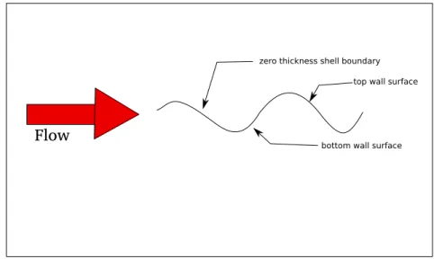
The shell boundary is basically a zero thickness interior face, treated as a double sided wall boundary condition as shown in Figure2-2. This allows for the modeling of prob- lems where it is undesirable for an immersed wall to have a thickness.
23 2.6. CLOSURE
zero thickness shell boundary top wall surface
bottom wall surface
Flow
Figure 2-2: Drawing of the shell boundary condition 2.5.2.5 Symmetric-Plane Boundary
At the symmetric boundary, the flow is expected to behave as if there is a mirror image of such flow on the other side of the plane. As a result, the velocity components normal to the boundary are set to zero and the normal gradient ofs the tangential components of the velocity are set to zero (slip boundary conditions ) . The normal gradient of the other scalar variables( namely the pressure, volume fraction, turbulence field variables) is also set to zero.
2.6 Closure
A mathematical model for the time dependent turbulent incompressible two-fluid flow have been presented in this chapter. The mathematical model is provided in conservative form for discretization using the finite volume method in the following chapter.
CHAPTER 2. MATHEMATICAL MODEL
Chapter 3
Numerical Method
Contents
3.1 Computation of Gradient . . . 26 3.2 Volume Fraction Equation . . . 31 3.3 The Momentum Equation . . . 33 3.4 Pressure-Velocity Coupling . . . 37 3.5 Turbulence . . . 40 3.6 Boundary Conditions . . . 42 3.7 Solution Procedure . . . 49 3.8 Closure . . . 49 This chapter presents the spatial and temporal discretization of the mathematical model presented in the previous chapter. The discretization method employed in this work is the well-established finite volume method[26,62, 91]. The co-located variable arrangement[26], where all flow field variables are defined at the cell center, is used.
This arrangement simplifies the implementation of the method into computer code and minimizes the connectivity and geometric information required by the the unstructured mesh. A segregated solution procedure is employed to solve set of non-linear equations.
25
The PISO algorithm is used to establish the pressure-velocity coupling and calculate the pressure. Finally, the numerical implementation of the boundary conditions is presented and the solution procedure is outline.
3.1 Computation of Gradient
A description of several methods that can used to estimate the gradient of a field is presented here. The methods vary in complexity, stencil size(number of cells used for the approximation ), and ability to handle arbitrary mesh topology ( i.e. orthogonal, skewed cell, and high-aspect ratio cells)
3.1.1 Green-Gauss Gradient
The Green-Gauss gradient method is one of the most widely used method to compute the gradient. The gradient is computed at cell-center as
(∇φ)P= 1
∆VP
∑
f
φfS~f (3.1)
whereφf is the face averaged value of the volume fraction (φ) which can be computed from several methods[26,62] with different stencil size.
3.1.1.1 Compact Stencil: Face-Averaged Green-Gauss Gradient
This method is known as a compact stencil method[26] where only the face neighbors of the cell are involved in the gradient computation as shown in Figure3-1. The face value (φf) is computed using the weighted average values of the two cells sharing the face as given by
φf = (1−λ)φP+λ φN (3.2)
27 3.1. COMPUTATION OF GRADIENT
P
Figure 3-1: Computational stencil of the Cell-based Green-Gauss gradient(Compact Stencil)
The interpolation factorλ can be computed using two methods:
Method 1
λ = |dP f|
|dP f|+|dN f| (3.3)
Method 2
λ =
S~f·dP f
S~f·dP f+S~f·dN f (3.4) In this work, the two methods were compared but the difference was found negligible for a well behaving mesh ( i.e. mesh that doesn’t include highly skewed cells) , so the first method is employed in all subsequent test cases.
The Face Averaged Green-Gauss method gives second order when the line con- necting the two cell centers (P) and (N) passes through the face center (f) , as shown in Figure3-1, which is the case in orthogonal meshes. An iterative correction is sometimes included to account for mesh non-orthogonality in badly conditioned mesh however the added computational cost is considerably high which makes it impractical for actual application.
CHAPTER 3. NUMERICAL METHOD
3.1.1.2 Extended Stencil: Node-Averaged Green-Gauss Gradient
This method is known as the extended stencil method[26] where the vertex neigh- bors(i.e. cells sharing at least a vertex ) of the cell are involved in the gradient com- putation as shown in Figure3-2.
P
Figure 3-2: Computational stencil of the Node-based Green-Gauss gradient(Extended Stencil)
First, the values at the vertices are computed using the inverse distance weighting as given by
φn=
∑
k∈NB(n) φk
|dkP|
∑
k∈NB(n) 1
|dkP|
(3.5)
wherenis the vertex node andNB(n)is the subset of cells surrounding vertexn.
The face value (φf) is then computed using the average values of the vertices values comprising the face f as given by Maric et al. [56]
φ∗f = 1 Nf v
∑
n∈f v(f)
φn (3.6)
where f v(f)is the subset of vertices comprising the face f andNf v is the number of
29 3.1. COMPUTATION OF GRADIENT vertices comprising the face .
In two dimensional computation, the face value (φf ) is set asφf =φ∗f . However, in three-dimensional, an additional step is added. The face is decomposed into triangles consisting of the face center and the two points on each the face edges as depicted in Figure3-3.
φf =
∑
t
wtφt (3.7)
wherewt is computed from
wt= At
∑t
At (3.8)
whereAt is the area of the triangle andφtis computed from
φt =1
3(φ∗f+φf v+φf v+1) (3.9)
This method adds two additional steps compared to the Face-Averaged method to pro-
f
Figure 3-3: Drawing of a decomposed three-dimensional face in the Node-based Green- Gauss gradient method
CHAPTER 3. NUMERICAL METHOD
vide a better approximation of the face valueφfthat accounts for mesh non-orthogonality without required additional mesh connectivity information. However, the method also implies repeated memory visits to the node values (φn) that are as many as the number of faces sharing the node/vertex which can be as high as 10 faces depending on the mesh.
For these reasons, this method is several times more computationally intensive than the Face-Averaged and so it must be employed only in situations where such accuracy is necessary.
3.1.2 Least Square Gradient
The least square gradient methods[62, 91] provides higher flexibility to obtain better accuracy at the cost of larger stencil size[63] as shown in Figure3-4.
The gradient components are computed by solving the following 3x3 system of equation
∑
k∈NB(P)
wk∆xk∆xk wk∆xk∆yk wk∆xk∆zk wk∆yk∆xk wk∆yk∆yk wk∆yk∆zk wk∆zk∆xk wk∆zk∆yk wk∆zk∆zk
(∂ φ∂x)P (∂ φ∂y)P (∂ φ
∂z)P
=
∑
k∈NB(P)
wk∆xk∆φk wk∆yk∆φk wk∆zk∆φk
(3.10) whereNB(P)is the subset of cells sharing a face ( compact stencil) or a vertex ( extended stencil) with the cellP.
The weightingwk is chosen such that neighboring cells closer to the cell P will having more influence on the gradient than farther cells. This particularly important when an extended stencil is employed to compute the gradient. For that purpose, thenth power inverse distance function, where the parameterncontrol the weighting, is a convenient and suitable choice. A higher value ofn means that the influence of the neighboring
31 3.2. VOLUME FRACTION EQUATION
P
Figure 3-4: Computational stencil of the Least-Square gradient (green: Compact Sten- cil, red: Extended Stencil)
cells closely located to cellPwould higher.
wk= 1
|dPk|n (3.11)
where|dPk|is the distance between neighboring cellkand the cellP.
A typical choice of n is 1 or 2. In this work, a compact stencil is employed and the parameter n was set 1.
3.2 Volume Fraction Equation
As previously described in Chapter2, the volume fraction (α) is defined as the ratio of the volume of fluid to the volume of the computational cell(P).
αp= Volume of fluid
Volume of the computational cell (3.12) CHAPTER 3. NUMERICAL METHOD
The finite volume discretization of the volume fraction advection equation (Equation (2.6)) is obtained by taking the volume integral of the equation over the control volume∆V.
I ∂ α
∂t dV+ I
∇·(α~V)dV = I
α∇·~V dV (3.13)
Assuming that the computational cell volumes doesn’t change throughout the computa- tions
I ∂ α
∂t dV =∂ α
∂t ∆V (3.14)
Applying Green’s theorem to the convective term (the second term on the left hand side) I
∇·(α~V)dV = I
S
α~v·dS~ =
∑
f
Fαf (3.15)
Similarly to the right hand side term I
α∇·~V dV =α I
S
~v·dS~ =αP
∑
f
F (3.16)
The discretized volume fraction equation can written as
∂ α
∂t ∆V+
∑
f
Fαf =αP
∑
f
F (3.17)
whereF is volumetric flux defined asF=~V·S~f,S~f is the area normal pointing out of the control volume, and the subscriptsPand f refer to the control volume and the faces of this volume respectively.
In this study, the time integration of the volume fraction was done using the third order Runge-Kutta Total Variation Diminishing (RK3) [29,80]. The computation of the face value of the volume fraction (αf) was done using the UMTHINC method which is presented in the next chapter.
![Figure 4-14: Flux polygon construction of the EMFPA[31, 55] approach and Jofre et al.](https://thumb-ap.123doks.com/thumbv2/123deta/9880702.1906220/94.892.130.714.298.655/figure-flux-polygon-construction-emfpa-approach-jofre-et.webp)