Instructions for use
T itle Harnack inequalities for supersolutions of fully nonlinear elliptic difference and differential equations
A uthor(s ) HA MA MUK I,NA O
C itation Hokkaido University Preprint S eries in Mathematics, 1065: 1-16
Is s ue D ate 2015-2-23
D O I 10.14943/84209
D oc UR L http://hdl.handle.net/2115/69869
T ype bulletin (article)
Harnack inequalities for supersolutions of fully nonlinear
elliptic difference and differential equations
Nao Hamamuki
∗February 22, 2015
Abstract
We present a new Harnack inequality for non-negative discrete supersolutions of fully nonlinear uniformly elliptic difference equations on rectangular lattices. This estimate applies to all supersolutions; instead the Harnack constant depends on the graph distance on lattices. For the proof we modify the proof of the weak Harnack inequality. Applying the same idea to elliptic equations in a Euclidean space, we also derive a Harnack type inequality for non-negative viscosity supersolutions.
Key words: Harnack inequality, Fully nonlinear elliptic equations, Discrete solutions, Viscosity solutions
Mathematics Subject Classification 2010: 35B05, 35J60, 65N22, 35D40
1
Introduction
We consider fully nonlinear, non-homogeneous second order equations of the form
F(D2u) =f(x) (1.1)
with a uniformly elliptic operatorF. A typical statement of the Harnack inequality is that there exists a constantC >0 such that the inequality
max
U u <=C {
min
U u+∥f∥Ln(V) }
(1.2)
holds for every non-negative solution u of (1.1) inV. Here V is a set which is (enough) larger than U, and n represents the dimension of space. One of well-known proofs of the Harnack inequality is a combination of a weak Harnack inequality, which asserts that, for somep >0,
∥u∥Lp(U)<=C
{
min
U u+∥f∥L
n(V)
}
holds for every non-negative supersolution u, and a local maximum principle (or a mean value inequality):
max
U u <=C {
∥u∥Lq(U)+∥f∥Ln(V)}
∗Department of Mathematics, Hokkaido University, Kita 10, Nishi 8, Kita-Ku, Sapporo, Hokkaido,
for subsolutionsu, whereq >0 is arbitrary. These estimates are well-known in the contin-uum case where (1.1) is studied as a partial differential equation in Rn; for instance, the
reader is referred to [9, Chapter 9] for linear equations and [3, Chapter 4] for fully nonlinear equations. The corresponding results are also obtained in the discrete case when we study (1.1) as a difference equation on lattices. In [13] the Harnack inequality for elliptic difference equations is derived via the weak Harnack inequality and the local maximum principle. See also [14] for the parabolic case and [15, 16] for general meshes.
The main goal of this paper is to show that, in the discrete case, a modified proof of the weak Harnack inequality implies a new type of the Harnack inequality for discrete supersolutions to (1.1) on rectangular lattices (Theorem 4.1). Our proof is direct and simple in the sense that we do not need the local maximum principle. The resulting estimate is different from the literature in that it holds for supersolutions which are not necessarily subsolutions; instead the Harnack constant, C in (1.2), depends on the graph distance on lattices. Due to this, passing to limits in our Harnack inequality does not imply the continuum Harnack inequality since the Harnack constantCgoes to infinity when the mesh size tends to 0 (Remark 3.4 and 4.2). Here it is worth to mention that such reconstruction of the continuum Harnack inequality should not be possible since (1.2) does not hold even for the Laplace equation if we do not requireuto be a subsolution; see Example 5.3 for the counter-example. We can say that our Harnack inequality is an interesting estimate which comes at the expense of convergence of discrete schemes.
In the proof of the weak Harnack inequality for fully nonlinear equations of the continuum case ([2, 3]), we take a radially symmetric and increasing supersolution ϕ of the Pucci equation
P−(D2ϕ) =−ξ(x). (1.3)
Here P− is a Pucci operator (see (5.2) or (2.2) for definition) and ξ is a non-negative,
continuous function whose support is contained in a small ball centered at the origin. Such a functionϕis often called abarrier function. In the discrete case, we are able to construct the barrier function so thatξis non-zero only at the origin (Lemma 3.1 and Remark 3.2). In other words, its support is only one point. This is a crucial difference from the continuous case, and this enables a pointwise estimate for supersolutions of difference equations. In our proof of the Harnack inequality, we translate the barrier function so that its minimum point, which originally lies at the origin, comes to a maximum point of the supersolutionuof (1.1). As a result, we obtain the Harnack inequality without discussing the local maximum principle.
We apply the same idea involving translation of the barrier function to partial differential equations in Rn. This gives our another result in this paper (Theorem 5.7). To describe the result, we first note that (1.2) can be stated equivalently as
u(z)<=C{min
U u+∥f∥Ln(V) }
for allz∈U, (1.4)
{|x−z|<=ε} is controlled by itsLp-norm on U. Thus the method in this paper presents
how a simple estimate is established by a simple argument without the Calder´on-Zygmund decomposition appearing in the literature ([2, 3]).
This paper is organized as follows: Section 2 is devoted to preparation for studies of difference equations on rectangular lattices. In Section 3 we construct a barrier functionϕ
in (1.3) so that the support ofξlies only at the origin. Then, in Section 4 we give a proof of the Harnack inequality for non-negative discrete supersolutions. Section 5 is concerned with the Harnack inequality inRn for viscosity supersolutions. We use a similar idea to the one presented in Section 4. In Appendix A we establish a unique existence of discrete solutions to Dirichlet problems of fully nonlinear uniformly elliptic difference equations. This unique solution is needed in Section 4 to derive the Harnack inequality with non-zerof.
2
Preliminaries
In this paper we consider ann-dimensional weighted latticehZn defined as
hZn:={(h1m1, . . . , hnmn)∈Rn |(m1, . . . , mn)∈Zn}.
Herehi is a fixed positive constant which represents a mesh size in the direction ofxi. We
set hmax := max{h1, . . . , hn} and hmin := min{h1, . . . , hn}. For Ω ⊂ hZn we define its
closure Ω⊂hZn and its boundary∂Ω⊂hZn as
Ω := Ω∪ {x±hiei |x∈Ω, i∈ {1, . . . , n}}, ∂Ω := Ω\Ω,
where{ei}ni=1⊂Rn is the standard orthogonal basis ofRn, e.g.,e1= (1,0, . . . ,0).
We next introduce difference operators. Let u:hZn →R, x∈hZn andi∈ {1, . . . , n}. We define the second order difference operators as follows:
δ2iu(x) :=
u(x+hiei) +u(x−hiei)−2u(x)
h2
i
, ⃗δ2u(x) := (δ2
1u(x), . . . , δ2nu(x)).
The difference equation we consider is
F(⃗δ2u(x)) =f(x), (2.1) whereF :Rn →Ris uniformly elliptic (Definition 2.2),F(0) = 0 andf :hZn→R.
Definition 2.1. Let Ω⊂hZn. We sayu: Ω→Ris adiscrete subsolution(resp. superso-lution) of (2.1) in Ω ifF(⃗δ2u(x))<
=f(x) (resp. >=f(x)) for allx∈Ω. Ifuis both a discrete sub- and supersolution, it is called adiscrete solution.
Throughout this paper we fix ellipticity constants 0< λ <= Λ. To describe the uniform
ellipticity ofF in (2.1) we introducePucci operatorsP±:Rn →R, which are defined as
P+(X⃗) :=−λ ∑ Xi>0
Xi−Λ ∑ Xi<0
Xi, P−(X⃗) :=−λ ∑ Xi<0
Xi−Λ ∑ Xi>0
Xi (2.2)
forX⃗ = (X1, . . . , Xn)∈Rn. An easy computation shows that the Pucci operators satisfy P−(X⃗ +Y⃗)<
Definition 2.2. We sayF :Rn →Risuniformly ellipticifP−(X⃗ −Y⃗)<
=F(X⃗)−F(Y⃗)<=
P+(X⃗ −Y⃗) for all X, ⃗⃗ Y ∈Rn.
PuttingY⃗ = 0, we see thatP−(X⃗)<
=F(X⃗)<=P+(X⃗) sinceF(0) = 0.
We next state the ABP maximum principle (ABP estimate). This is a pointwise estimate for subsolutions and supersolutions of elliptic equations, and it will be used in the proof of the Harnack inequality. We prepare some notations before stating the estimate. Fora∈R
we seta± := max{±a,0} (>
= 0). Let Ω⊂hZn and u: Ω→R. We define ΓΩ[u], anupper
contact setofuon Ω, as
ΓΩ[u] :=
{
x∈Ω
there exists somep∈Rn such that
u(y)<=⟨p, y−x⟩+u(x) for all y∈Ω
}
, (2.3)
where ⟨·,·⟩is the standard Euclidean inner product in Rn. The p-norm (p∈[1,∞)) of u
over Ω is given as∥u∥ℓp(Ω):=
(∑
x∈Ωhn|u(x)|p
)1/p
, wherehn:=h
1× · · · ×hn. We only use
the casep=nin this paper. The diameter of Ω is diam(Ω) := maxx∈Ω,y∈∂Ω|x−y|. Here
| · |stands for the standard Euclidean norm inRn.
Theorem 2.3(ABP maximum principle). LetΩ⊂hZnbe bounded. There exists a constant
CA=CA(n, λ)>0such that, for every discrete subsolution (resp. supersolution)uof(2.1) inΩ, the estimate
max
Ω
u <= max
∂Ω u ++C
Adiam(Ω)∥f+∥ℓn(ΓΩ[u+]) (2.4)
(resp. min
Ω
u >= min
∂Ω(−u
−)−C
Adiam(Ω)∥f−∥ℓn(ΓΩ[u−])) (2.5)
holds.
We do not give a proof of Theorem 2.3; see [13, Theorem 2.1], [10, Theorem 4.1].
3
Barrier function
In the proof of the Harnack inequality we use a barrier function, which is a radially increasing supersolution ofP− = 0 except at the origin. (See [3, Lemma 4.1] for the continuum case.)
Forx∈hZn given asx= (h
1m1, . . . , hnmn) with (m1, . . . , mn)∈Zn, we defineρ(x) := |m1|+· · ·+|mn|. This represents the graph distance on hZn between 0 andx, i.e., the
number of edges in a shortest path connecting them. Let k ∈ N∪ {0}. We define a ball
Bk ⊂hZn as Bk :={x∈hZn |ρ(x)<=k}, which is a diamond-shaped set. Note that the
indexk is not the Euclidean distance but the graph distance.
Lemma 3.1 (Barrier function). Let k∈N. There exists a functionϕ:Bk →Rsuch that
P−(⃗δ2ϕ)>
= 0 in Bk\ {0}, (3.1)
ϕ= 0 on ∂Bk, (3.2)
ϕ <=−1 in Bk. (3.3)
Proof. Let{am}km+1=0 ⊂R. We define ϕ(x) := am ifρ(x) = m ∈ {0,1, . . . , k+ 1} and set
ak+1= 0,ak =−1. We show that, for givenam+1 andamsuch that am+1> am, we have P−(⃗δ2ϕ(x))>
Fixm∈ {1, . . . , k}andx= (x1, . . . , xn)∈Bk\ {0}such thatρ(x) =m. Let us calculate
δ2
iϕ(x). Ifxi= 0, we observe
δ2
iϕ(x) =
am+1+am+1−2am
h2
i
= 2(am+1−am)
h2
i
>0.
On the other hand, ifxi ̸= 0, then
δi2ϕ(x) =
am+1+am−1−2am
h2
i
,
which is negative whenam−1≪ −1. Thus the definition ofP− implies that
P−(⃗δ2ϕ(x)) =−λ∑ xi̸=0
δ2iϕ(x)−Λ ∑ xi=0
δ2iϕ(x).
Now, there exists at least one indexisuch thatxi̸= 0 sincex̸= 0. Therefore
P−(⃗δ2ϕ(x))>
=−λam+1+ha2m−1−2am max
−Λ2(am+1−am)
h2 min
(n−1)
=− λ
h2 max
(
am+1+am−1−2am+2Λh
2
max(n−1)(am+1−am)
λh2 min
)
. (3.4)
This is non-negative if am−1 ≪ −1, and hence (3.1) holds. The conditions (3.2) and (3.3)
are clear by construction.
Remark3.2. Using the barrier functionϕin Lemma 3.1, we define
ξ(x) :=
{
−P−(⃗δ2ϕ(0)) ifx= 0,
0 ifx̸= 0.
Then ϕis a supersolution of P− =−ξ in B
k. We also note that ξ(0) >0 sinceδ2iϕ(0) =
2(a1−a0)/h2i >0 for alli= 1, . . . , n.
Remark3.3. In view of the proof, we notice thatϕ(0) depends onk, n,Λ/λandhmax/hmin.
The positive constant−ϕ(0) will appear as the Harnack constantCH in (4.2).
Remark 3.4. The quantity in parentheses of (3.4) is chosen to be non-positive, and so we haveam+1−am< am−am−1form∈ {1, . . . , k}. This yieldsa0<−k−1 sinceak+1−ak = 1.
It thus follows that the valueϕ(0) =a0goes to−∞ask→ ∞. This implies that we cannot
obtain the continuum Harnack inequality as the limit of our discrete Harnack inequality; see Remark 4.2.
4
Harnack inequality
We show the Harnack inequality for non-negative discrete supersolutions of
P+(⃗δ2u) =−f−(x). (4.1)
Theorem 4.1 (Harnack inequality). Let r ∈ N. Then there exists a constant CH =
CH(r, n,Λ/λ, hmax/hmin) >0 such that, for every non-negative discrete supersolution u :
B3r→[0,∞) of(4.1)inB3r, the estimate
max
Br
u <=CH {
min
Br
u+CAdiam(B3r)∥f−∥ℓn(B3 r)
}
(4.2)
holds, whereCA is the constant in Theorem 2.3.
We first prove (4.2) in the case when f− ≡0; a crucial difference between the discrete
case and the continuum case appears in this part. We translateξin Remark 3.2 so that its support comes to a maximum point ofu and derive the estimate foru at the point. The proof for a general f is similar to the proof in the continuum case; see, e.g., [1, Proof of Theorem 1.11]. We employ a solutionvof a Pucci equation and study u+v to apply (4.2) withf−≡0.
Proof. Case: f− ≡0. 1. We take x
M, xm∈ Br such thatu(xM) = maxBruand u(xm) = minBru. Our goal is to deriveu(xM)<=CHu(xm). Letϕbe the barrier function in Lemma 3.1 withk= 2r. Letβ > u(xm) (>= 0). We defineϕ˜(x) :=βϕ(x−xM) and
˜
ξ(x) :=
{
−P−(⃗δ2ϕ˜(x
M)) if x=xM,
0 ifx̸=xM.
Set B :=xM +B2r. Then Br ⊂B ⊂B3r since xM ∈ Br. By virtue of Lemma 3.1 and
Remark 3.2, we have
P−(⃗δ2ϕ˜)>
=−ξ˜ in B, (4.3)
˜
ϕ= 0 on ∂B, (4.4)
˜
ϕ <=−β in B. (4.5) 2. Let us study a function u+ ˜ϕ. For everyx∈B we deduce from (4.3) that
P+(⃗δ2u(x) +⃗δ2ϕ˜(x))>=P+(⃗δ2u(x)) +P−(⃗δ2ϕ˜(x))>= 0−ξ˜(x).
Namely,u+ ˜ϕis a supersolution of P+=−ξ˜inB. Applying the ABP maximum principle
(2.5) tou+ ˜ϕ, we obtain min
B (u+ ˜ϕ)>= min∂B{−(u+ ˜ϕ) −} −C
Adiam(B)∥ξ˜∥ℓn(ΓB[(u+ ˜ϕ)−]). (4.6)
Sinceuis non-negative and (4.4) holds, we haveu+ ˜ϕ >= 0 on ∂B, and thus min∂B{−(u+
˜
ϕ)−}= 0. As for the left-hand side of (4.6), using (4.5), we compute
min
B (u+ ˜ϕ)<= minB u−β <= minBr
u−β <0.
Therefore it follows from (4.6) that 0>−∥ξ˜∥ℓn(ΓB[(u+ ˜ϕ)−]). Since ˜ξis nonzero only atxM
by its definition, we must have
xM ∈ΓB[(u+ ˜ϕ)−]. (4.7)
3. We claim (u+ ˜ϕ)(xM) < 0. Suppose by contradiction that (u+ ˜ϕ)(xM) >= 0, i.e.,
(u+ ˜ϕ)−(x
M) = 0. Then, since (u+ ˜ϕ)−= 0 on∂B, (4.7) implies
Indeed, by (4.7) there exists somep= (p1, . . . , pn)∈Rn such that
0<= (u+ ˜ϕ)−(y)<= (u+ ˜ϕ)−(xM) +⟨p, y−xM⟩=⟨p, y−xM⟩ (4.9)
for ally∈B. Fixi∈ {1, . . . , n}and choosek+, k− ∈Nsuch thatxM±k±hiei ∈∂B. (Such
numbersk± exist sinceB is bounded.) Takingy=xM ±k±hiei in (4.9), we observe
0<=⟨p, k+hiei⟩=k+hipi, 0<=⟨p,−k−hiei⟩=−k−hipi,
which implypi = 0. Finally, applyingp= 0 to (4.9) yields (4.8). However, at a minimum
pointxmwe have (u+ ˜ϕ)(xm)<=u(xm)−β <0. This contradicts to (4.8).
By the claim we have u(xM) < −ϕ˜(xM) = −βϕ(0), and sending β → u(xm) yields
u(xM)<=CHu(xm) withCH=−ϕ(0).
Case: f−̸≡0. 1. Letvbe the discrete solution of
{
P−(⃗δ2v) =f− inB
3r,
v= 0 on∂B3r.
We will prove a unique existence of solutions in Appendix A (Theorem A.4) for more general Dirichlet problems. By the ABP maximum principles we see thatv satisfies
max
B3r
v <= max
∂B3r
v++C
Adiam(B3r)∥(f−)+∥ℓn(Γ B3r[v+])
<
= 0 +CAdiam(B3r)∥f−∥ℓn(B3
r) (4.10)
and
min
B3r
v >= min
∂B3r
(−v−)−C
Adiam(B3r)∥(f−)−∥ℓn(ΓB
3r[v−])
= 0−0. (4.11)
2. We now consider a function u+v. By the non-negativity of uand (4.11), we have
u+v >= 0 inB3r. Next, for x∈B3rwe compute
P+(⃗δ2u(x) +⃗δ2v(x))>
=P+(⃗δ2u(x)) +P−(⃗δ2v(x))>=−f−(x) +f−(x) = 0. Thusu+vis a non-negative supersolution ofP+= 0 inB
3r. From the Harnack inequality
of the casef− ≡0 it follows that
max
Br
(u+v)<=CHmin Br
(u+v).
Finally, applying the estimates (4.10) and (4.11) to the right- and the left-hand side respec-tively, we obtain (4.2).
Remark 4.2. Passing to limits in (4.2) as h→0 does not imply the Harnack inequality in the continuum case. Indeed, to derive the continuum Harnack inequality on a bounded set
K⊂Rn, one needs to “cover”Kby a discrete ballBr⊂hZn. When the mesh size goes to
0, the radius r∈N must tend to infinity, and thus the valueCH =−ϕ(0) goes to infinity
5
Continuum case
We consider elliptic partial differential equations of the form
F(D2u(x)) =f(x), (5.1) where D2u(x) = (∂2
iju(x))ij denotes the Hessian matrix, F ∈ C(Sn) is uniformly elliptic
(Definition 5.2), F(O) = 0 and f ∈ C(Rn). Here Sn is the set of real n×n symmetric matrices. In this section, applying the idea of the proof of Theorem 4.1, we deduce a Hanack type inequality for supersolutions of (5.1).
We employ a notion of viscosity solutions to solve (5.1) since it is fully nonlinear.
Definition 5.1. Let Ω⊂Rnbe open. We say thatu∈C(Ω) is aviscosity subsolution(resp.
supersolution) of (5.1) in Ω ifF(D2ϕ(x))<
=f(x) (resp. >=f(x)) for all (x, ϕ)∈Ω×C2(Ω) such thatu−ϕattains a local maximum (resp. minimum) atx.
For given ellipticity constants 0< λ <= Λ we definePucci operatorsP±:Sn→Ras
P+(X) :=−λ∑
µi>0
µi−Λ ∑ µi<0
µi, P−(X) :=−λ ∑ µi<0
µi−Λ ∑ µi>0
µi, (5.2)
whereµi (i= 1, . . . , n) are the eigenvalues of X∈Sn. It is easily seen that these operators
satisfyP−(X+Y)<
=P+(X) +P−(Y)=<P+(X+Y) for all X, Y ∈Sn. We also have
P+(X) = sup{−trace(AX)|A∈Sn, λI <=A <= ΛI},
P−(X) = inf{−trace(AX)|A∈Sn, λI <=A <= ΛI},
i.e., P± are Bellman type operators. Here I is the identity matrix, and forX, Y ∈Sn we
writeX <=Y if⟨(Y −X)ξ, ξ⟩>= 0 for allξ∈Rn.
Definition 5.2. We sayF :Sn→Risuniformly ellipticifP−(X−Y)<
=F(X)−F(Y)<=
P+(X−Y) for all X, Y ∈Sn.
Now, we shall give examples showing that the usual Harnack inequality does not hold in the continuum case if we requireuto be only a non-negative supersolution. In this section
Brstands for the open ball{|x|< r}inRn. The closure of it inRnis denoted byBr. Also,
setBr(z) :={|x−z|< r}.
Example 5.3. We consider the Laplace equation −∆u = 0 in Rn when n >= 3. Set u(x) = min{c|x|2−n, 1} with c > 0. As is known, |x|2−n is the fundamental solution of
the Laplace equation while any constant is trivially a solution. Since the minimum of two supersolutions is still a supersolution ([5, Lemma 4.2]),uis a viscosity supersolution. On the other hand,uis not a viscosity subsolution. Indeed, lettingϕ(x) =−ε|x|2forε >0 small, we
see thatu−ϕtakes a maximum at a pointzsuch thatc|z|2−n= 1, but−∆ϕ(z) = 2nε >0.
Now, let us fixr >0. We then have maxBru= 1 and minBru=cr2−nforcsmall. Thus the
ratio (maxBru)/(minBru) tends to∞as c→0. This implies that the Harnack inequality does not hold.
The functionsu(x) = min{|x|2−n, M}withM >0 also show that the Harnack inequality
does not hold by lettingM →0.
We state the ABP maximum principle for viscosity solutions. Let Ω⊂Rn be an open set andu: Ω→R. Similarly to the discrete case, we define a upper contact set ΓΩ[u] by
(2.3). Set∥u∥Ln(Ω):= (
∫
Theorem 5.4(ABP maximum principle). LetΩ⊂Rn be a bounded open set. There exists a constantCA=CA(n, λ)>0such that, for every viscosity subsolution (resp. supersolution)
u∈C(Ω)of (5.1)inΩ, the estimate
max
Ω
u <= max
∂Ω u ++C
Adiam(Ω)∥f+∥Ln(ΓΩ[u+]) (5.3)
(resp. min
Ω u >= min∂Ω(−u
−)−C
Adiam(Ω)∥f−∥Ln(ΓΩ[u−])) (5.4)
holds.
For the proof see [4, Proposition 2.12, Appendix A] or [11, Proposition 6.2, Section 7.2]. To present a barrier function in the continuum case, we first prepare
Lemma 5.5. Let 0< ρ < Rand defineψ(x) :=M1−M2|x|−α with
M1=
R−α
ρ−α−R−α, M2=
1
ρ−α−R−α, α= max {
1, (n−1)Λ λ −1
}
.
Then
P−(D2ψ)>
= 0 inRn\ {0},
ψ >= 0 inRn\BR,
ψ <=−1 inBρ.
(5.5)
Proof. See [3, Lemma 4.1].
Let ε >0. We say that a functionω : [0, ε]→[0,∞) is amoduluson [0, ε] ifω(0) = 0, limr→0ω(r) = 0 andω is non-decreasing on [0, ε].
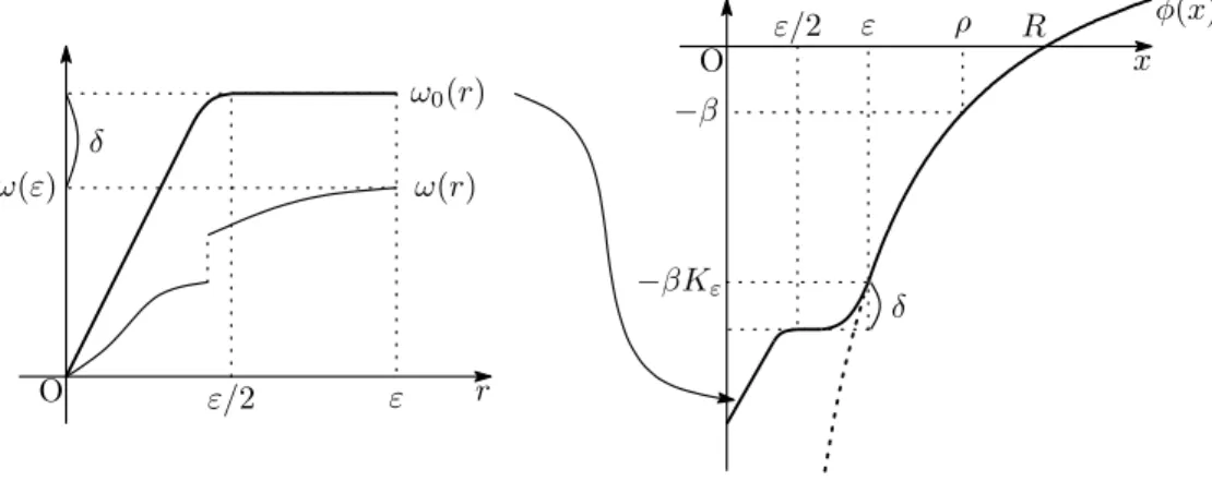
Lemma 5.6. Let ω be a modulus on [0, ε]. Let δ >0. Then there exists a modulusω0 on
[0, ε] such thatω0∈C2(0, ε),ω0> ω on(0, ε] andω0(r) =ω(ε) +δ for allr∈[ε/2, ε].
Proof. We set ω1(0) := 0, ω1(ε) = ω1(ε/2) := ω(ε) +δ and ω1(ε/2j+1) := ω(ε/2j) for
j∈N. On each interval [ε/2j, ε/2j−1] we interpolateω
1by a linear function. Then ω1 is a
modulus such thatω1>=ω on [0, ε]. We next define ω2(r) := min{2ω1(r), ω(ε) +δ}, which
is again a piecewise linear modulus satisfying ω2 > ω on (0, ε] and ω0(r) = ω(ε) +δ for
allr∈[ε/2, ε]. Finally, mollifying ω2 near each corner of the graph, we obtain the desired
C2-functionω 0.
A similar technique to make a smooth modulus can be found in [8, Lemma 2.1.9]. Using the above functions, let us construct a barrier function which will be used in the proof of our Harnack inequality. Let 0< ε < ρ < Randω be a modulus on [0, ε]. We also give positive constants β, δ > 0. Set Kε := −(M1−M2ε−α) > 0, which will appear as the Harnack
constantCH in (5.9). We define
ϕ(x) :=
{
βψ(x) if|x|>=ε, ω0(|x|)−βKε−2δ−ω(ε) if|x|<=ε/2.
On{ε/2<=|x|<=ε}we extendϕsmoothly so thatϕ∈C2(Rn\ {0}) and−βK
O x ε
ε/2 ρ R
−β
−βKε
δ
O ε r
ω(r)
ω0(r)
δ
φ(x)
ε/2
ω(ε)
Figure 1: The graphs ofω0 andϕ.
the following properties:
P−(D2ϕ)>
= 0 inRn\Bε,
ϕ >= 0 inRn\BR,
ϕ <=−β inBρ
(5.6)
and
ϕ(x)−ϕ(0)> ω(|x|) if 0<|x|<=ε. (5.7) Since ϕ is not necessarily a C2-function on the whole space, we next mollify it near the
origin. For j ∈ N we mollify ϕ in Bε/2j so that ϕj ∈ C2(Rn), ϕj <= −β in Bρ and ϕj
converges to ϕuniformly in Rn as j → ∞. Then eachϕ
j satisfies the three properties in
(5.6). We next defineξj(x) :=|P−(D2ϕj(x))|. It then follows that P−(D2ϕ
j)>=−ξj(x) in Rn, supp(ξj)⊂Bε.
Here supp(ξj) :={x∈Rn |ξj(x)̸= 0}.
We now derive the Harnack inequality for viscosity supersolutions of
P+(D2u) =−f−(x). (5.8)
A viscosity supersolution of (5.1) is always a supersolution of (5.8).
Theorem 5.7 (Harnack inequality). Let r > 0 and 0 < ε < 2r. Then there exists a constantCH =CH(r, ε, n,Λ/λ)>0such that, for every non-negative viscosity supersolution
u∈C(B4r)of (5.8)inB4r, the estimate
min
Bε(z)
u <=CH {
min
Br
u+CAdiam(Ω)∥f−∥Ln(B4r)
}
(5.9)
holds for allz∈Br, whereCA is the constant in Theorem 5.4. Proof. Case: f− ≡0. 1. Fix anyz ∈B
r. Fort∈[0, ε] we defineω(t) :=u(z)−minBt(z)u.
Br, i.e.,u(xm) = minBru, and letβ > u(xm) (>= 0). We takeϕ, ϕj andξj as the functions
given after Lemma 5.6 withρ= 2randR= 3r, whereω andβ are chosen as above. Define ˜
ϕ(x) :=ϕ(x−z),ϕ˜j(x) :=ϕj(x−z) and ˜ξ(x) :=ξ(x−z). We furthermore setB′:=B2r(z)
andB:=B3r(z), so that we haveBr⊂B′⊂B⊂B4r.
By (5.7) we see that u+ ˜ϕ attains its strict minimum at z over Bε(z). Indeed, if
0<|x−z|<=ε, we compute
u(x) + ˜ϕ(x)>{u(z)−ω(|x−z|)}+{ϕ˜(z) +ω(|x−z|)}=u(z) + ˜ϕ(z).
We letzj be a minimum point ofu+ ˜ϕj overBε(z). Then, since ˜ϕj uniformly converges to
˜
ϕ, it follows thatzj →zas j→ ∞.
2. We show that u+ ˜ϕj is a viscosity supersolution of P+ =−ξ˜j in B. Assume that
u+ ˜ϕj−ψattains a local minimum atx∈Bforψ∈C2(B). Sinceu+ ˜ϕj−ψ=u−(ψ−ϕ˜j)
anduis a viscosity supersolution of (5.8), we observe
0<=P+(D2ψ(x)−D2ϕ˜j(x))<=P+(D2ψ(x))− P−(D2ϕ˜j(x))
<
=P+(D2ψ(x)) + ˜ξj(x),
which implies the assertion. Therefore the ABP maximum principle (5.4) implies
min
B (u+ ˜ϕj)
>
= min∂B{−(u+ ˜ϕj)−} −CAdiam(B)∥ξ˜j∥Ln(ΓB[(u+ ˜ϕj)−]).
Similarly to the discrete case, we have min∂B{−(u+ ˜ϕj)−} = 0 and minB(u+ ˜ϕj)<0 by
the properties of ˜ϕj, and hence ∥ξ˜j∥Ln(Γ
B[(u+ ˜ϕj)−]) > 0. Since supp( ˜ξj) ⊂ Bε(z), we see
that the setBε(z)∩ΓB[(u+ ˜ϕj)−] is not empty.
3. Choose an arbitrary y ∈Bε(z)∩ΓB[(u+ ˜ϕj)−]. Then we see (u+ ˜ϕj)(y)<0 by a
similar argument to the discrete case. Sinceu+ ˜ϕj attains its minimum atzj overBε(z), it
follows that
u(zj) + ˜ϕj(zj)=<u(y) + ˜ϕj(y)<0.
Lettingj→ ∞, we have
u(z)<=−ϕ˜(z) =−ϕ(0) =βKε+ 2δ+ω(ε).
By the definition ofω, this gives min
Bε(z)
u <=βKε+ 2δ.
Finally, sendingβ→u(xm) andδ→0 yield minBε(z)u <=CHu(xm) withCH =Kε.
Case: f−̸≡0. 1. Let {f
j}∞j=1 ⊂C∞(Rn) be a sequence of smooth functions such that
fj >=f− inB4r for allj∈Nand that fj converges tof− uniformly onB4r asj→ ∞. We
consider the Dirichlet problem
{
P−(D2v
j) =fj inB4r,
vj = 0 on∂B4r
(5.10)
and denote by vj ∈ C2(B4r)∩C(B4r) the solution of (5.10). The existence of smooth
type) equations. See [6, 7, 12] or [11, Section 7.3]. The ABP maximum principles, (5.3) and (5.4), yield
0<=vj<=CAdiam(Ω)∥fj∥Ln(B
4r) onB4r. (5.11) 2. Now, it is easy to see thatu+vj is a viscosity solution ofP+= 0 inB4r. Sinceu+vj
is non-negative onB4r by (5.11), the Harnack inequality (5.9) withf−≡0 implies
min
Bε(z)
(u+vj)<=CHmin Br
(u+vj).
Applying the first and the second inequality in (5.11) to the left- and the right-hand side of the above estimate respectively, we obtain
min
Bε(z)
u <=CH {
min
Br
u+CAdiam(Ω)∥fj∥Ln(B4r)
}
.
Sendingj → ∞gives (5.9).
Remark5.8. The estimate (5.9) we established can be written as
u(z)<=CH {
min
Br
u+CAdiam(Ω)∥f−∥Ln(B4r)
}
+ω(ε),
which gives a pointwise estimate foru, but the right-hand side involves a modulus of conti-nuity from below ofuaroundz.
Remark 5.9. The functions in Example 5.3 shows that the Harnack constant CH in (5.9)
must go to infinity when ε → 0. Indeed, the Harnack constant which we selected in the proof isCH=Kε=−(M1−M2ε−α) and this tends to infinity asε→0.
As a byproduct of this observation, we see non-existence of a radially symmetric function
ψ∈C(Rn)∩C2(Rn\ {0}) satisfying the three conditions in (5.5). (Note that the function
ψin Lemma 5.5 does not belong toC(Rn).) If there were such aψ, by a similar argument to the proof of Theorem 5.7 we would have the Harnack inequality (5.9) withCH which is
less than−ψ(0), a contradiction.
Remark5.10. The result in Theorem 5.7 still holds forLp-viscosity solutions, although we do
not give the details in this paper. In the theory ofLp-viscosity solutions,f is just assumed
to be in Lp(Ω) and solutions are defined by test functions belonging toW2,p
loc. In this case,
we do not need to approximate f− by smooth functions f
j in the proof of the Harnack
inequality because the Dirichlet problem (5.10) withf− instead off
j admits a solution in
Wloc2,p. Also, it is not difficult to extend the result to more general equations of the form
P+(D2u) +µ|Du|=−f−(x)
with µ >= 0. See [4] and [11, Section 6 and 7] for the theory of Lp-viscosity solutions and
the above generalized equation.
A
A well-posedness of uniformly elliptic equations
We prove that the Dirichlet problem
F(⃗δ2u(x)) =f(x) in Ω, (A.1)
has a unique discrete solution. Here Ω⊂hZn is a bounded set, F :Rn →Ris uniformly
elliptic,F(0) = 0,f : Ω→Randg:∂Ω→Ris a given boundary datum. The uniqueness easily follows from the ABP maximum principle. The existence of solutions to elliptic difference equations is more or less known even when the equation is degenerate; for example, the fixed point theorem is one of powerful tools to show the existence. However, we present it here to make the paper self-contained and to give the proof based onPerron’s method, which cannot be found much in discrete problems.
For X, ⃗⃗ Y ∈ Rn given as X⃗ = (X1, . . . , Xn) and Y⃗ = (Y1, . . . , Yn), we write X <⃗ =Y⃗ if
Xi <=Yi for all i∈ {1, . . . , n}. By the uniform ellipticity of F, we have F(X⃗) >=F(Y⃗) if
⃗
X <=Y⃗. This is a degenerate ellipticity ([5, (0.3)]).
From the ABP maximum principle (Theorem 2.3) we immediately deduce a compari-son principle for a discrete sub- and supersolution of (A.1). This implies a uniqueness of solutions.
Corollary A.1(Comparison principle). Letuandv be, respectively, a discrete subsolution and supersolution of(A.1). Ifu <=v on ∂Ω, then u <=v in Ω.
Proof. SinceF is uniformly elliptic, we observe
P−(⃗δ2u(x)−⃗δ2v(x))<
=F(⃗δ2u(x))−F(⃗δ2v(x))<=f(x)−f(x) = 0
for allx∈Ω. Thereforeu−v is a discrete subsolution of the Pucci equationP−= 0 in Ω.
We now apply the ABP maximum principle to obtain maxΩ(u−v)<= max∂Ω(u−v)<= 0.
We turn to an existence problem. To construct discrete solutions, we employ the idea of Perron’s method for viscosity solutions ([5, Section 4]).
Proposition A.2 (Perron’s method). Let v and V be, respectively, a discrete sub- and supersolution of(A.1) such that v <=V onΩ. Let
S:=
{
w: Ω→R
wis a discrete subsolution of(A.1)
such that v <=w <=V on Ω
}
.
Thenu(x) := supw∈Sw(x)is a discrete solution of(A.1).
Proof. 1. We first prove that u is a discrete subsolution. Fix x∈ Ω and ε > 0. By the definition ofuthere exists somewε∈ S such thatu(x)−ε <=wε(x)<=u(x). We then observe
δi2u(x) =
u(x+hiei) +u(x−hiei)−2u(x)
h2
i
>
= wε(x+hiei) +wε(xh−2hiei)−2(wε(x) +ε)
i
=δ2iwε(x)− 2ε
h2
i
for eachi∈ {1, . . . , n}. Thus
⃗δ2u(x)>
=⃗δ2wε(x)− 2ε
h2 min
From the uniform ellipticity ofF it follows that
F(⃗δ2u(x))<=F
(
⃗δ2w
ε(x)− 2ε
h2 min
(1, . . . ,1)
)
<
=F(⃗δ2wε(x))− P− (
2ε h2
min
(1, . . . ,1)
)
=F(⃗δ2wε(x)) + Λ
2εn h2
min
. (A.3)
We now have F(⃗δ2w
ε(x))<= f(x) since wε ∈ S. Applying this to (A.3) and then letting
ε→0, we obtainF(⃗δ2u(x))<
=f(x). This implies thatuis a discrete subsolution.
2. We next show thatuis a discrete supersolution. Suppose that this were false. Then we could find somey∈Ω such that
F(⃗δ2u(y))< f(y). (A.4)
For suchyandδ >0 we define
U(x) :=
{
u(y) +δ ifx=y, u(x) ifx̸=y.
We claim thatU ∈ Sfor a sufficiently smallδ >0. Showing this claim yields a contradiction sinceU is strictly larger thanuat y.
We first prove u(y)< V(y). Supposeu(y) =V(y). Then, noting that u(x)<=V(x) for
x̸= y, we would have⃗δ2u(y) <
=⃗δ2V(y). SinceV is a supersolution, it would follow that
F(⃗δ2u(y))>
=F(⃗δ2V(y))=>f(y), a contradiction to (A.4). Thusv <=U <=V on Ω if we take
δ <=V(y)−u(y).
Let us show that U is a subsolution. Letx∈Ω. It is easily seen that⃗δ2U(x) =⃗δ2u(x)
ifx̸∈ {y}and that⃗δ2U(x)>
=⃗δ2u(x) ifx∈ {y} \ {y}. Therefore the ellipticity ofF implies thatF(⃗δ2U(x))<
=F(⃗δ2u(x))<=f(x) forx̸=y. We next consider the casex=y. Then
δi2U(y) =
u(y+hiei) +u(y−hiei)−2(u(y) +δ)
h2
i
=δ2iu(y)−
2δ h2
i
,
and so the same calculation as in Step 1 yields
F(⃗δ2U(y))<=F(⃗δ2u(y)) + Λ2δn
h2 min
=f(y) + Λ2δn
h2 min
− {f(y)−F(⃗δ2u(y))}.
In view of (A.4), it follows thatF(⃗δ2U(y)) <
=f(y) if δ <= h2min{f(y)−F(⃗δ2u(y))}/(2Λn).
Summarizing the above argument, we conclude that U ∈ S, and hence u is a discrete supersolution.
Example A.3. Let A = (A1, . . . , An) ∈ Rn. We define a quadratic function q = qA :
hZn → Ras q(x) := ∑n
j=1Ajx2j for x= (x1, . . . , xn)∈ hZn. Then δi2q is a constant for
eachi∈ {1, . . . , n}. Indeed, we observe
δ2
iq(x) =
q(x+hiei) +q(x−hiei)−2q(x)
h2
i
=Ai(xi+hi)
2+A
i(xi−hi)2−2Aix2i
h2
i
= 2Ai
for allx∈hZn. In particular, if we takeAi=−c/(2λn) withc >= 0, then
P−(⃗δ2q(x)) =−λ· −c
λn·n=c,
i.e.,qis a discrete solution of the above Pucci equation in hZn.
Theorem A.4(Unique solvability). The Dirichlet problem(A.1)and(A.2)admits a unique discrete solution.
Proof. The uniqueness is a consequence of the comparison principle, Corollary A.1. To show the existence we constructvandV in the statement of Proposition A.2 such thatv=V =g
on∂Ω; then Proposition A.2 ensures thatu:= supw∈Swis a discrete solution of (A.1) and
(A.2). To construct suchv and V we use quadratic functions in Example A.3. Let qA be
the quadratic function in Example A.3 withAi=−(maxΩ|f|)/(2λn), so that
P−(⃗δ2qA(x)) = max
Ω |f| in Ω. (A.5)
Choosek >= 0 such that qA+k >= max∂Ωg on Ω, and define
V(x) :=
{
qA(x) +k ifx∈Ω,
g(x) ifx∈∂Ω.
Then V is a discrete supersolution of (A.1). Indeed, since V <= qA+k on ∂Ω, we have
⃗δ2V(x) <
= ⃗δ2(qA+k)(x) = ⃗δ2qA(x) for x ∈ Ω. Therefore it follows from ellipticity that
F(⃗δ2V(x)) >
= F(⃗δ2qA(x)) >= P−(⃗δ2qA(x)). By virtue of (A.5) we conclude that V is a
discrete supersolution of (A.1).
Similarly, using a suitable quadratic function, we are able to construct a discrete subso-lutionvwhich satisfiesv=gon∂Ω andv <= min∂Ωgin Ω. The proof is now complete since
v <= min∂Ωg <= max∂Ωg <=V in Ω.
Acknowledgments
The work of the author was suppoted by Grant-in-aid for Scientific Research of JSPS Fellows No. 23-4365 and No. 26-30001.
References
[2] L. A. Caffarelli, Interior a priori estimates for solutions of fully nonlinear equations, Ann. of Math. (2) 130 (1989), no. 1, 189–213.
[3] L. A. Caffarelli, X. Cabr´e, Fully nonlinear elliptic equations, American Mathematical Society Colloquium Publications, vol. 43, American Mathematical Society, Providence, RI, 1995.
[4] L. A. Caffarelli, M. G. Crandall, M. Kocan, A. Swi¸ech, On viscosity solutions of fully nonlinear equations with measurable ingredients, Comm. Pure Appl. Math. 49 (1996), no. 4, 365–397.
[5] M. G. Crandall, H. Ishii, P. L. Lions, User’s guide to viscosity solutions of second order partial differential equations, Bull. Amer. Math. Soc. (N.S.) 27 (1992), no. 1, 1–67.
[6] L. C. Evans, Classical solutions of fully nonlinear, convex, second-order elliptic equa-tions, Comm. Pure Appl. Math. 35 (1982), no. 3, 333–363.
[7] L. C. Evans, Classical solutions of the Hamilton-Jacobi-Bellman equation for uniformly elliptic operators, Trans. Amer. Math. Soc. 275 (1983), no. 1, 245–255.
[8] Y. Giga, Surface evolution equations: A level set approach, Monographs in Mathemat-ics, 99, Birkhauser Verlag, Basel, 2006, xii+264 pp.
[9] D. Gilbarg, N. S. Trudinger, Elliptic partial differential equations of second order, Reprint of the 1998 edition, Classics in Mathematics, Springer-Verlag, Berlin, 2001.
[10] N. Hamamuki, A discrete isoperimetric inequality on lattices, Discrete Comput. Geom. 52 (2014), no. 2, 221–239.
[11] S. Koike, A beginner’s guide to the theory of viscosity solutions, MSJ Memoirs, 13. Mathematical Society of Japan, Tokyo, 2004, viii+123 pp.
[12] N. V. Krylov, Boundedly nonhomogeneous elliptic and parabolic equations, Izv. Akad. Nauk SSSR Ser. Mat. 46 (1982), 487–523 (Russian); English translation in Math. USSR Izv. 20 (1983), 459–492.
[13] H.-J. Kuo, N. S. Trudinger, Linear elliptic difference inequalities with random coeffi-cients, Math. Comp. 55 (1990), no. 191, 37–53.
[14] H.-J. Kuo, N. S. Trudinger, Local estimates for parabolic difference operators, J. Dif-ferential Equations 122 (1995), no. 2, 398–413.
[15] H.-J. Kuo, N. S. Trudinger, Positive difference operators on general meshes, Duke Math. J. 83 (1996), no. 2, 415–433.