RIMS-1754
On the a posteriori estimates for inverse operators of linear parabolic equations with applications to
the numerical enclosure of solutions for nonlinear problems
By
Takehiko KINOSHITA, Takuma KIMURA, and Mitsuhiro T. NAKAO
July 2012
R ESEARCH I NSTITUTE FOR M ATHEMATICAL S CIENCES
KYOTO UNIVERSITY, Kyoto, Japan
On the a posteriori estimates for inverse operators of linear parabolic equations with applications to the numerical enclosure of solutions for nonlinear problems
Takehiko Kinoshita · Takuma Kimura · Mitsuhiro T. Nakao
July 24, 2012
Abstract We consider the guaranteed a posteriori estimates for the inverse parabolic operators with homogeneous initial-boundary conditions. Our estimation technique uses a full-discrete numerical scheme, which is based on the Galerkin method with an interpolation in time by using the fundamental solution for semidiscretization in space. In our technique, the constructive a priori error estimates for a full discretiza- tion of solutions for the heat equation play an essential role. Combining these esti- mates with an argument for the discretized inverse operator and a contraction prop- erty of the Newton-type formulation, we derive an a posteriori estimate of the norm for the infinite-dimensional operator. In numerical examples, we show that the pro- posed method should be more efficient than the existing method. Moreover, as an application, we give some prototype results for numerical verification of solutions of nonlinear parabolic problems, which confirm the actual usefulness of our technique.
Keywords Parabolic PDEs·Galerkin methods·A posteriori estimates·Numerical verification methods
Mathematics Subject Classification (2000) 35K20·65M15·65M60
1 Introduction
SettingLt:=∂∂t−ν4+b·∇+c, for f∈L2(
J;L2(Ω)), consider the following linear parabolic partial differential equations (PDEs) with homogeneous initial and bound-
Takehiko Kinoshita
Research Institute for Mathematical Sciences, Kyoto University, Kyoto 606-8502, Japan E-mail: [email protected]
Takuma Kimura
JST CREST / Faculty of Science and Engineering, Waseda University, Tokyo 169-8555, Japan E-mail: [email protected]
Mitsuhiro T. Nakao
Sasebo National College of Technology, Nagasaki 857-1193, Japan E-mail: [email protected]
ary conditions:
Ltu=f, inΩ×J, (1a)
u(x,t) =0, on∂Ω×J, (1b)
u(x,0) =0, inΩ, (1c)
whereΩ ⊂Rd,(d∈ {1,2,3})is a bounded polygonal or polyhedral domain,J:=
(0,T)⊂R,(T<∞)is a bounded interval,νis a positive constant,b∈L∞(
J;L∞(Ω))d, andc∈L∞(
J;L∞(Ω)). As is well known, for any f ∈L2(
J;L2(Ω)), there exists a unique weak solution u∈L2(
J;H01(Ω))to the problem (1). Denoting the solu- tion operator of (1) byLt−1, it is a bounded linear operator from L2(
J;L2(Ω))to L2(
J;H01(Ω)).
The main aim of this paper is to obtain the concrete valueCL2L2,L2H01>0 satisfying the following estimates:
Lt−1
L(L2(J;L2(Ω)),L2(J;H01(Ω)))≤CL2L2,L2H01. (2) The constantCL2L2,L2H01plays an important role in the verification of solutions for the initial-boundary-value problems for the nonlinear parabolic PDEs, and we usually need to estimate it as small as possible. The concrete valueCL2L2,L2H01 >0 satisfying (2) can be calculated by the Gronwall inequality or other theoretical considerations (e.g., [16]), which we call the “a priori estimates.” However, in general,CL2L2,L2H01
obtained by such a priori estimates is exponentially dependent on the length of the time intervalJunless the corresponding elliptic part of the operatorLtis coercive [4, 5]. Thus a priori estimates often lead to an overestimate for the norm ofLt−1, which yields worse results for some purposes.
In order to overcome this difficulty, we proposed a method to calculateCL2L2,L2H01
by numerical computation with guaranteed accuracy in [10], which we called “a pos- teriori estimates.” The method is based on combining the a priori error estimates for a semidiscretization with the a priori estimates for the ordinary differential equations (ODEs) in time. It has proven to be more efficient than the existing a priori method;
some numerical examples show that this a posteriori method can remove the expo- nential dependency on the time intervalJ. However, it has a very large computational cost, because the semidiscretization of (1) causes stiff ODEs that require a very small step size. Also, it is not clear what time-space ratio to use in the discretization process.
In this paper, we propose a new a posteriori method with a fully discretized Newton-type operator, which uses the Galerkin approximation in the space direction and the Lagrange-type interpolation in the time direction. In the case of the simple heat equations, some fundamental properties (e.g., the stability and a priori error es- timates) for this full-discretization scheme have already been obtained in [11]. In the desired estimation of the inverse operator normLt−1
L(L2(J;L2(Ω)),L2(J;H01(Ω))), the matrix norm estimates corresponding to the discretized inverse operator and the constructive error analysis for the simple heat equations are important and essential.
By constructive analysis, we can also guess an appropriate time-space ratio prior to the actual computation. Moreover, by using numerical examples, we will show that
the proposed method succeeds in obtaining a posteriori estimates with less computa- tional cost than the previous method in [10]. This means that the present method is very robust compared with the previous one.
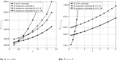
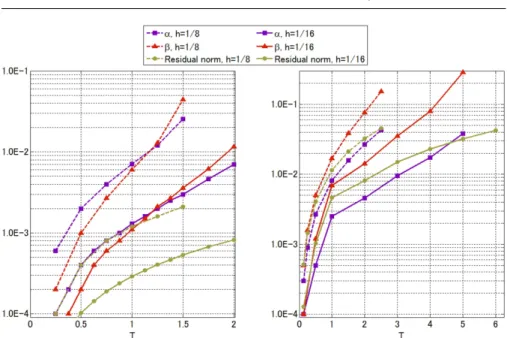
The contents of this paper are as follows: In section 2, we introduce some function spaces, operators, and other notation. In section 3, we introduce the results of stabil- ity and a priori error estimates for the full-discretization scheme for the simple heat equations, which were obtained in [11]. In section 4, we consider the approximate quasi-Newton operator that corresponds to the full-discretization scheme for prob- lem (1). In section 5, we derive the new a posteriori estimates of (2) by combining the results in section 3 with the property of the approximate quasi-Newton operator defined in the previous section. In section 6, we compare the computed values for CL2L2,L2H01 by three methods, namely, the a priori method, the a posteriori estimates in [10], and the new a posteriori method obtained in section 5. In this section we also show some prototype results of the numerical enclosure of solutions for nonlinear parabolic problems as an application of our method.
2 Notation
In this section, we introduce some function spaces, operators, and other notation. Let L2(Ω)andH1(Ω)be the usual Lebesgue and Sobolev spaces onΩ, respectively, and define the natural inner product ofu,vinL2(Ω)by(u,v)L2(Ω):=∫Ωu(x)v(x)dx.
Also, letH01(Ω)be a Sobolev space defined byH01(Ω):={u∈H1(Ω);u=0 on∂Ω} with inner product(u,v)H1
0(Ω):= (∇u,∇v)L2(Ω)d. We will sometimes refer to the fol- lowing Sobolev inequality onH01(Ω). Namely, for a suitable constant p≥1, which is dependent on the dimension ofΩ, there exists a constantCs,p>0 such that
kukLp(Ω)≤Cs,pkukH1
0(Ω), ∀u∈H01(Ω). (3)
Whenp=2, (3) is called the Poincar´e inequality.
Let4:L2(Ω)→L2(Ω)be the Laplace operator that is self-adjoint on the domain D(4):={
u∈H01(Ω);4u∈L2(Ω)}. LetV1(J)be a subspace ofH1(J)defined by V1(J):={
u∈H1(J);u(0) =0}
. Then,V1(J)is a Hilbert space with inner product (u,v)V1(J):= (u0,v0)L2(J). The time-dependent Lebesgue space L2(
J;L2(Ω))is de- fined as a space of square-integrableL2(Ω)-valued functions onJ. Then,L2(
J;L2(Ω)) is a Hilbert space with inner product(u,v)L2(J;L2(Ω)):=∫J∫Ωu(x,t)v(x,t)dxdt. We denote the function space L2(
J;L2(Ω))asL2L2, for short. Let L2(
J;H01(Ω))be a subspace ofL2L2defined by
L2(
J;H01(Ω)):={u∈L2L2; ∇u∈L2(
J;L2(Ω))d, u(·,t) =0 on∂Ω,a.e.t∈J }
. Then, L2H01 ≡L2(
J;H01(Ω)) is a Hilbert space with inner product (u,v)L2H01 :=
(∇u,∇v)(L2L2)d. LetV1(
J;L2(Ω))be a subspace ofL2L2defined by V1(
J;L2(Ω)):=
{ u∈L2(
J;L2(Ω)); ∂u
∂t ∈L2
(J;L2(Ω)), u(·,0) =0 inL2(Ω) }
.
Then,V1L2≡V1(
J;L2(Ω))is a Hilbert space with inner product(u,v)V1L2:=
(∂u
∂t,∂∂vt )
L2L2. We define the Hilbert spaceV:=V1L2∩L2H01with inner product(u,v)V:= (u,v)V1L2+ (u,v)L2H01 =
(∂u
∂t,∂∂vt )
L2L2+ (∇u,∇v)(L2L2)d. Moreover, we define the partial differ- ential operator4t:L2L2→L2L2by4t:=∂∂t−ν4on the domainD(4t):=V1L2∩ L2(
J;D(4))
. Then, the inverse of4t exists (e.g., [3]), and we denote it by4−1t ∈ L(L2L2). Notably, the range of4−1t satisfiesR(4−1t ) =D(4t). From the compact- ness of the embeddingIe:D(4t),→L2H01, the bounded linear operatorIe4−1t ∈ L(L2L2,L2H01)is also compact.
Let Sh(Ω) be a finite-dimensional subspace of H01(Ω) dependent on the dis- cretization parameter h. For example, Sh(Ω) is considered to be a finite element space with mesh sizeh. Let nbe the number of degrees of freedom ofSh(Ω), and let{φi}ni=1⊂H01(Ω)be the basis functions ofSh(Ω). Moreover, we denote a vector of the basis functions ofSh(Ω)byφ:= (φ1, . . . ,φn)T. We also assume the inverse estimates onSh(Ω)like as follows:
Assumption 2.1 There exists a positive constant Cinv(h)satisfying kuhkH1
0(Ω)≤Cinv(h)kuhkL2(Ω), ∀uh∈Sh(Ω). (4) For example, ifΩ is a bounded open interval inR, andSh(Ω)is the P1 finite ele- ment space, then Assumption 2.1 is realized withCinv(h) =
√12
hmin, wherehmin is the minimum mesh size in the division ofΩ (see e.g., [15, Theorem 1.5]).
LetPh1:H01(Ω)→Sh(Ω)be anH01-projection. Namely, for an arbitrary element u∈H01(Ω),Ph1u∈Sh(Ω)satisfies the following variational equation:
(∇(u−Ph1u),∇vh)
L2(Ω)d =0, ∀vh∈Sh(Ω). (5) We need the following assumptions as the a priori error estimates forPh1.
Assumption 2.2 There exists a positive constant CΩ(h)satisfying u−Ph1u
H01(Ω)≤CΩ(h)k4ukL2(Ω), ∀u∈D(4), (6) u−Ph1u
L2(Ω)≤CΩ(h)u−Ph1u
H01(Ω), ∀u∈H01(Ω). (7) For example, ifΩis a bounded open interval inR, andSh(Ω)is the P1 finite element space, then Assumption 2.2 is realized asCΩ(h) =πh, wherehis the mesh size (see e.g., [1, 7]).
LetVk1(J)be a finite-dimensional subspace ofV1(J)dependent on the discretiza- tion parameterk. For example,Vk1(J)is considered to be a finite element space with mesh size (time step size)k. Letmbe the number of degrees of freedom forVk1(J), and let{ψi}mi=1⊂V1(J)be the basis functions ofVk1(J). Moreover, we denote a vec- tor of the basis functions ofVk1(J)byψ:= (ψ1, . . . ,ψm)T.
We assume thatΠk:V1(J)→Vk1(J)is a Lagrange interpolation operator. Namely, if the mesh points onJ are taken as 0=t0<t1<···<tm=T, for any element u∈V1(J),Πku∈Vk1(J)satisfies
u(ti) =( Πku)
(ti), ∀i∈ {1, . . . ,m}. (8) We need the following assumption as the a priori error estimate forΠk.
Assumption 2.3 There exists a positive constant CJ(k)satisfying
ku−ΠkukL2(J)≤CJ(k)kukV1(J), ∀u∈V1(J). (9) For example, ifVk1(J)is the P1 finite element space, then Assumption 2.3 is realized byCJ(k) =πk (see e.g., [15, Theorem 2.4]).
LetV1(
J;Sh(Ω))andVk1
(J;Sh(Ω))be the semidiscretization and the full-discretization subspaces ofV, respectively. We now define the semidiscretization operatorPh:V→ V1(
J;Sh(Ω))by the following weak form for anyu∈V (∂
∂t
(u−Phu) (t),vh
)
L2(Ω)
+ν(∇(
u−Phu)
(t),∇vh)
L2(Ω)d =0,
∀vh∈Sh(Ω), a.e. t∈J. (10) Then the full-discretization operatorPh,k:V→Vk1(
J;Sh(Ω))is defined as the com- position ofPhandΠk, that is, byPh,k:=ΠkPh.
3 Constructive a priori error estimates
In this section, we introduce some results for the stability of, and a priori error es- timates for, the full-discretization operatorPh,k. Since the results of this section are given in [11], we omit the proofs.
Theorem 3.1 ([11, Lemma 5.3 & Theorem 5.4]) Under Assumption 2.1 and Assump- tion 2.3, the following constructive a priori estimate holds,
Ph,ku
L2(
J;H01(Ω))≤ (Cs,2
ν +Cinv(h)CJ(k) )∂u
∂t −ν4u L2L2
, ∀u∈D(4t).
(11) Moreover, if Vk1(J)is the P1 finite element space then we have the following estimates:
Ph,ku
V1(
J;L2(Ω))≤2 ∂u
∂t −ν4u L2(
J;L2(Ω)), ∀u∈D(4t). (12) Since the full-discretization scheme proposed in [6, 9] has noV1L2stability, we can say that the present full-discretized approximation has better properties, in an analyt- ical and practical sense.
Finally, we introduce the constructive a priori error estimates forPh,k.
Theorem 3.2 ([11, Theorem 5.5 & Theorem 5.6]) Under the assumptions 2.1- 2.3, we have the following constructive a priori error estimates:
u−Ph,ku
L2(
J;H01(Ω))≤C1(h,k) ∂u
∂t −ν4u L2(
J;L2(Ω)), ∀u∈D(4t), (13) u−Ph,ku
L2(
J;L2(Ω))≤C0(h,k) ∂u
∂t −ν4u L2(
J;L2(Ω)), ∀u∈D(4t), (14) where C1(h,k):=2νCΩ(h) +Cinv(h)CJ(k)and C0(h,k) =8νCΩ(h)2+CJ(k).
4 Discretized quasi-Newton scheme
In this section, we consider a full-discretized approximation scheme for solutions of (1) by using a quasi-Newton operator. Since the full-discretization scheme in this paper uses interpolation in time, its computational method is somewhat complicated.
However, it enables us to get an efficient and accurate estimation of the inverse opera- tor norm in (2), as well as the verified computation of solutions to nonlinear problems.
We first describe an easy, but an important operation of matrix-vector multiplica- tion.
Definition 4.1 Let M be an m1-by-m2matrix. Then, we define the m1m2vector vec(M) as follows:
vec(M):= (M1,1,M1,2, . . . ,M1,m2,M2,1, . . . ,Mm1,m2)T. (15) We call this transformation a “row-major matrix-vector transformation”.
Definition 4.2 Let M be an m1-by-m2 matrix. Then, we define the block diagonal matrix(In⊗M)as follows:
(In⊗M):=
M ··· 0
... . .. ... 0 ··· M
| {z }
n
. (16)
Here, In is the n-by-n identity matrix, and the operator⊗denotes the Kronecker product.
From these definitions, we have the following lemma.
Lemma 4.3 For an arbitrary n-by-m matrix M and m-dimensional vector x, the fol- lowing equality holds:
Mx=( In⊗xT)
vec(M). (17)
Proof. —— The elements ofMxare calculated by
Mx=
M1,1··· M1,m ... . .. ... Mn,1··· Mn,m
x1
... xm
=
M1,1x1+···+M1,mxm ...
Mn,1x1+···+Mn,mxm
.
On the other hand, the elements of( In⊗xT)
vec(M)are calculated by (In⊗xT)
vec(M) =
xT ··· 0 ... . .. ... 0 ··· xT
M1,1
... Mn,m
=
M1,1x1+···+M1,mxm ...
Mn,1x1+···+Mn,mxm
.
Therefore, the corresponding components coincide with each other.ut
Next, we consider the quasi-Newton operator of (1) and its full-discretization.
LetAbe an integral operator defined byA:=−Ie4t−1(b·∇+c):L2(
J;H01(Ω))→ L2(
J;H01(Ω)). Since the domain of4t isD(4t), denoting the range ofAbyR(A), it holds thatR(A)⊂D(4t) =V1L2∩L2D(4). Then, the differential operator of the left-hand side of (1a) can be represented as Lt =4t(I−A), whereI denotes the identity operator onD(4t). We define the quasi-Newton operator as the inverse of I−A, i.e.,(I−A)−1:L2H01→L2H01.
We now define the symmetric and positive definite matricesLφ andDφ∈Rn×n by
Lφ,i,j:= (φj,φi)L2(Ω), Dφ,i,j:= (∇φj,∇φi)L2(Ω)d, ∀i,j∈ {1, . . . ,n}. LetL1/2φ andD1/2φ be the Cholesky factors ofLφandDφ, respectively, i.e., the follow- ing equalities hold
Lφ=L1/2φ LTφ/2, Dφ=D1/2φ DT/2φ ,
whereL1/2φ andD1/2φ are lower triangular matrices, andLT/2φ andDT/2φ are those matri- ces transposed. LetLψ∈Rm×mbe the symmetric and positive-definite matrix whose elements are defined byLψ,i,j:= (ψj,ψi)L2(J). We defineZφ∈L∞(J)n×nas the matrix function onJwhose elements are defined by
Zφ,i,j:= ((b·∇)φj+cφj,φi)L2(Ω), ∀i,j∈ {1, . . . ,n}.
For anyi∈ {1, . . . ,m}, we define the matrices ˜G(i)φ,ψ∈Rn×nmand ˜Gφ,ψ∈Rnm×nmby
G˜(i)φ,ψ:=
∫ ti 0
exp (
(s−ti)νLφ−1Dφ
)
L−1φ Zφ(s)(
In⊗ψ(s)T)ds, G˜φ,ψ:=
G˜(1)φ,ψ
... G˜(m)φ,ψ
.
(18) Moreover, we defineGφ,ψ∈Rnm×nmasGφ,ψ:=Inm−G˜φ,ψ.
We obtain the Theorem 4.4 as a full-discretization scheme of the quasi-Newton operator.
Theorem 4.4 Let Vk1(J)be a finite element space constituted by the Lagrange ele- ments. For a function fh,k∈Vk1(
J;Sh(Ω)), let uh,k∈Vk1(
J;Sh(Ω))be a solution of the following equation
uh,k−Ph,kAuh,k=fh,k. (19) Then, the unique existence of a solution uh,kof(19)is equivalent to the nonsingularity of Gφ,ψ.
Proof. —— First, we considerPh,kAuh,k. For an arbitraryuh,k∈Vk1(
J;Sk(Ω)), there exists a matrixU∈Rn×msuch thatuh,k(x,t) =φ(x)TUψ(t). Letwh:=PhAuh,k. Sim- ilarly, fromwh∈V1(
J;Sh(Ω)), there exists a vector functionw∈V1(J)nsuch that wh(x,t) =φ(x)Tw(t) =
∑
ni=1
φi(x)wi(t).
For eachvh∈Sh(Ω), and almost everywheret∈J, from the definition ofPhand the operatorA, we have
(∂wh
∂t (t),vh )
L2(Ω)
+ν(∇wh(t),∇vh)L2(Ω)d
=
(∂Auh,k
∂t (t),vh )
L2(Ω)
+ν(∇Auh,k(t),∇vh)
L2(Ω)d,
=((
b(t)·∇)
uh,k(t) +c(t)uh,k(t),vh)
L2(Ω). (20) From the arbitrariness ofvh∈Sh(Ω), the variational equation (20) is equivalent to the following system of first-order linear ODEs with homogeneous initial conditions
( Lφd
dt+νDφ
)
w=ZφUψ. (21) Since (21) is an initial-value problem for an ODE system with constant coefficients, by using its fundamental matrix,wcan be presented as
w(t) =
∫ t 0
exp (
(s−t)νL−1φ Dφ
)
L−1φ Zφ(s)Uψ(s)ds (22)
= (∫ t
0
exp (
(s−t)νL−1φ Dφ
)
L−1φ Zφ(s)(
In⊗ψ(s)T)ds )
vec(U), (23) where we have used (17) to make the deformation from (22) to (23). And, from (18), we have
w(ti) =G˜(i)φ,ψvec(U)∈Rn, ∀i∈ {1, . . . ,m}. (24) Thus, from (23), we obtain the following relation betweenUandw:
(w(t1)T, . . . ,w(tm)T)T
=G˜φ,ψvec(U).
Now, we prove that if (19) is solvable for each fh,k∈Vk1(
J;Sh(Ω)), thenGφ,ψ
is nonsingular. For an fh,k∈Vk1(
J;Sh(Ω)), we denote the solution of (19) asuh,k∈ Vk1(
J;Sh(Ω)). From the fact that fh,k∈Vk1Sh, there exists an F∈Rn×m such that fh,k(x,t) =φ(x)TFψ(t). Note that, for any nodal pointsti, we have(Ph,kAuh,k)(x,ti) =
(Πkwh)(x,ti) =φ(x)Tw(ti)by the definition ofΠk. Therefore, from (19) and (24), we have
uh,k(x,ti)−fh,k(x,ti) = (Ph,kAuh,k)(x,ti), ∀x∈Ω,∀i∈ {1, . . . ,m},
= (Πkwh)(x,ti), which implies
φ(x)T(U−F)ψ(ti) =φ(x)Tw(ti)
=φ(x)TG˜(i)φ,ψvec(U). (25) Since we assume thatVk1(J)is the finite element space constituted by the Lagrange elements,ψj(ti) =δj,iis satisfied, whereδj,idenotes the Kronecker delta. Therefore, we get
(U−F)ψ(ti) =
U1,1−F1,1··· U1,m−F1,m ... . .. ... Un,1−Fn,1··· Un,m−Fn,m
ψ1(ti)
... ψm(ti)
=
U1,i−F1,i ... Un,i−Fn,i
.
From the arbitrariness of xandi, the variational equation (25) is equivalent to the following simultaneous linear equations:
vec(U−F) =G˜φ,ψvec(U). Namely, we have
(Inm−G˜φ,ψ)
vec(U) =vec(F).
Therefore, from the arbitrariness of fh,k, the nonsingularity ofInm−G˜φ,ψfollows.
The converse of this proposition is easily obtained by reversing the discussion.ut When we apply the proposed a posteriori estimates, it is necessary to confirm thatGφ,ψis nonsingular, which will be able to verify by validated computations such as [14]. Therefore, in what follows, we always assume the nonsingularity ofGφ,ψ. Moreover, we define the linear operator[I−A]−1h,k:Vk1(
J;Sh(Ω))→Vk1(
J;Sh(Ω))by the solution of (19). We call this operator a “fully discretized quasi-Newton operator”.
5 A posteriori estimates
In this section, we derive a new a posteriori estimate to obtainCL2L2,L2H01, which satisfies (2) by using the fully discretized quasi-Newton operator.
First, we describe a method to calculate the norm of the elements in the full- discretization space. LetKφ,ψbe a matrix inRnm×nmdefined by
Kφ,ψ:=Dφ⊗Lψ=
Dφ,1,1Lψ ··· Dφ,1,nLψ ... . .. ... Dφ,n,1Lψ ··· Dφ,n,nLψ
. (26)
From the symmetric positive definiteness ofDφ andLψ, it is readily seen thatKφ,ψis also symmetric positive definite. Therefore,Kφ,ψis Cholesky decomposable such that Kφ,ψ=Kφ1/2,ψKφT,/2ψ. Similarly, we define the matrixLφ,ψinRnm×nmasLφ,ψ:=Lφ⊗Lψ. Lemma 5.1 For an element uh,k∈Vk1(
J;Sh(Ω)), taking U∈Rn×msuch that uh,k= φTUψ, then the following equalities hold
uh,k
L2(
J;L2(Ω))=LφT,/2ψvec(U), (27) uh,k
L2(
J;H01(Ω))=KφT/2,ψvec(U), (28) where| · |denotes the Euclidean norm of a vector.
Proof. —— Since the proofs of (27) and (28) are almost the same, we will prove only (27). From (17), we have
uh,k2
L2(
J;L2(Ω))=
∫ J
∫
Ωψ(t)TUTφ(x)φ(x)TUψ(t)dxdt
=
∫ J
∫
Ωvec(U)T(In⊗ψ(t))Tφ(x)φ(x)T(In⊗ψ(t)T)vec(U)dxdt
=vec(U)T
∫ J
(In⊗ψ(t))TLφ(
In⊗ψ(t)T)dtvec(U)
=vec(U)T
∫ J
Lφ,1,1ψ(t)ψ(t)T ··· Lφ,1,nψ(t)ψ(t)T ... . .. ... Lφ,n,1ψ(t)ψ(t)T ··· Lφ,n,nψ(t)ψ(t)T
dtvec(U)
=vec(U)T
Lφ,1,1Lψ··· Lφ,1,nLψ ... . .. ... Lφ,n,1Lψ··· Lφ,n,nLψ
vec(U)
= (
LTφ,/2ψvec(U) )T(
LT/2φ,ψvec(U) )
, which proves equation (27).ut
LetMφ,ψ(h,k)be a nonnegative constant defined byMφ,ψ(h,k):=KφT/2,ψG−1φ,ψKφ−T/2,ψ
2, wherek · k2denotes the matrix two-norm. The following theorem forMφ,ψholds.
Theorem 5.2 It holds that [I−A]−1h,kfh,k
L2(
J;H01(Ω))≤Mφ,ψfh,k
L2(
J;H01(Ω)), ∀fh,k∈Vk1Sh. (29) Proof. —— For any fh,k∈Vk1Sh, we setuh,k:= [I−A]−1h,kfh,k∈Vk1Sh. Since fh,kand uh,k are the elements ofVk1(
J;Sh(Ω)), there exist matrices F andU inRn×m such that fh,k=φTFψ anduh,k=φTUψ, respectively. Moreover, from the proof of The- orem 4.4, it follows that vec(U) =G−1φ,ψvec(F). Therefore, we have the following
estimates uh,k2
L2(
J;H01(Ω))=vec(U)TKφ,ψvec(U)
= (
KφT/2,ψvec(U) )T(
KφT/2,ψG−φ,1ψKφ−T/2,ψ )(
KφT,/2ψvec(F) )
≤uh,k
L2(
J;H01(Ω))KφT/2,ψG−1φ,ψKφ−T/2,ψ
2
fh,k
L2(
J;H01(Ω)). This completes the proof.ut
LetC0andC1be the nonnegative constants defined by C0:=Mφ,ψ
(Cs,2
ν +Cinv(h)CJ(k) )
, C1:=kbkL∞L∞+Cs,2kckL∞L∞, respectively. Moreover, we define the constantκφ,ψas follows:
κφ,ψ:=kbkL∞L∞(1+C0C1)C1(h,k) +C0C1C0(h,k)kckL∞L∞
1−C0(h,k)kckL∞L∞
, (30)
provided that 1−C0(h,k)kckL∞L∞6=0.
Theorem 5.3 Assume that
0≤κφ,ψ<1. (31)
Then under the same assumptions as in Theorem 3.2, we have the following construc- tive a posteriori estimates
Lt−1
L(
L2(J;L2(Ω)),L2(J;H01(Ω)))≤ 1 1−κφ,ψ
C0+ (1+C0C1)C1(h,k) 1−C0(h,k)kckL∞L∞
. (32)
Proof. —— For any f ∈L2(
J;L2(Ω)), we setu:=Lt−1f ∈D(4t). Then we make the following decomposition of (1) into two parts, e.g., the finite- and infinite-dimensional parts, using the projectionPh,k. Namely, in the spaceL2(
J;H01(Ω)), using the follow- ing equivalency
∂u
∂t −ν4u+ (b·∇)u+cu=f
⇐⇒u=Ie4−1t (
−(b·∇)u−cu+f)
, (33)
we have the decomposition:
⇐⇒
{ Ph,ku=Ph,kIe4−1t (
−(b·∇)u−cu+f)
, (34a)
(I−Ph,k)u= (I−Ph,k)Ie4−1t (
−(b·∇)u−cu+f)
. (34b)
We setu⊥:=u−Ph,kufor short. From (34a), using the definition of the operatorA, we have
Ph,ku=Ph,k(
A(Ph,ku+u⊥) +Ie4−1t f) ,