DECISION PROCESSES WITH UNKNOWN TRANSITION MATRICES
by
TetsuichiroIki, Masayuki Horiguchi, Masami Yasuda and
MasamiKurano
Reprinted from the Bulletin of Informatics and Cybernetics Research Association of Statistical Sciences,Vol.39
- r¾ ¾- r¾
-FUKUOKA, JAPAN 2007
A LEARNING ALGORITHM FOR
COMMUNICATING MARKOV DECISION
PROCESSES WITH UNKNOWN TRANSITION
MATRICES
ByTetsuichiroIki∗, MasayukiHoriguchi†, MasamiYasuda‡ and
MasamiKurano§
Abstract
This study is concerned with finite Markov decision processes (MDPs) whose state are exactly observable but its transition matrix is unknown. We develop a learning algorithm of the reward-penalty type for the communicating case of multi-chain MDPs. An adaptively optimal policy and an asymptotic sequence of adaptive policies with nearly optimal properties are constructed under the average expected reward criterion. Also, a numerical experiment is given to show the practical effectiveness of the algorithm.
Key Words and Phrases: Adaptive policy, Average case, Communicating case, Learning algo-rithm, Markov decision processes, Reward-penalty type, Unknown transition matrix.
1. Introduction and notation
In the real world, there are many requests to solve uncertain models. Adaptive mod-els for uncertain Markov decision processes (MDPs) have been considered by many au-thors as Hern´andez (1989), Hern´andez/ Marcus (1985), Kurano (1972), Kurano (1983), Mandl (1974), Martin (1967), van Hee (1978) and so on. The idea of Neuro dynamic programming by Bertsekas/Tsitsiklis (1996) is powerful in treating the adaptive MDPs. However, a simple learning algorithm of the reward-penalty type, investigated by Lakshmivarahan (1981) and Meybodi/Lakshmivarahan (1982) are more comprehensible and manageable. Kurano (1987) proposed a learning algorithms of the reward-penalty type where all elements of the true transition matrices of finite MDPs are known to be positive and constructed adaptively optimal policy under the average expected reward criterion.
In this paper, applying the idea of Kurano (1987) to a wider class of uncertain MDPs, we develop a learning algorithm for the communicating case of multi-chain MDPs
∗Faculty of Education and Culture, Miyazaki University, Miyazaki 889-2192 Japan,
†General Education, Yuge National College of Maritime Technology, Ehime 794-2593 Japan,
‡Faculty of Science, Chiba University, Chiba 263-8522 Japan, [email protected] §Faculty of Education, Chiba University, Chiba 263-8522 Japan, [email protected]
and construct an adaptively average optimal policy for a class of perturbed communi-cating MDPs. For general communicommuni-cating MDPs, an asymptotic sequence of adaptive policies with nearly optimal properties is constructed by using the results of perturbed case.
In the reminder of this section, we will formulate finite MDPs whose transition matrices are unknown but the state at each stage is observable exactly. Consider a controlled dynamic system with finite state and action spaces, S and A, containing
N <∞ and K < ∞ elements respectively. Let Q denote the parameter space of K
unknown stochastic matrices, that is Q ={q = (qij(a))¯¯¯ qij(a)= 0,
∑
j∈S
qij(a) = 1 for i, j∈ S, a ∈ A }
.
The sample space is the product space Ω = (S× A)∞ such that the projections
Xt, ∆t on the t-th factors S, A describe the state and action at the t-th stage of the process(t = 0). Let Π denote the set of all policies, i.e., for π = (π0, π1, . . .)∈ Π, let
πt∈ P (A|(S ×A)t×S) for all t = 0, where, for any finite sets X and Y , P (X|Y ) denotes
the set of all conditional probability distribution on X given Y . A policy π = (π0, π1, . . .)
is called randomized stationary if a conditional probability γ = (γ(·|i) : i ∈ S) ∈ P (A|S) such that πt(·|x0, a0, . . . , xt) = γ(·|xt) for all t= 0 and (x0, a0, . . . , xt)∈ (S × A)t× S.
Such a policy is simply denoted by γ. We denote by F the set of functions on S with
f (i)∈ A for all i ∈ S. A randomized stationary policy γ is called stationary if there
exists a function f ∈ F with γ({f(i)}|i) = 1 for all i ∈ S, which is denoted simply by f. We will construct a probability space as follows: For any initial state X0= i, π∈ Π
and a transition law q = (qij(a)) ∈ Q, let P (Xt+1 = j|X0, ∆0, . . . , Xt = i, ∆t = a) = qij(a) and P (∆t= a|X0, ∆0, . . . , Xt= i) = πt(a|X0, ∆0, . . . , Xt= i) (t= 0). Then, we
can define the probability measure Pπ(·|X0= i, q) on Ω. For a given reward function r
on S× A, we shall consider the long-run expected average reward:
ψ(i, q|π) = lim inf T→∞ 1 T + 1Eπ (∑T t=0 r(Xt, ∆t)¯¯¯ X0= i, q ) (1.1)
where Eπ(·|X0= i, q) is the expectation operator with respect to Pπ(·|X0= i, q).
LetD be a subset of Q. Then, the problem is to maximize ψ(i, q|π) over all π ∈ Π for any i∈ S and q ∈ D. Thus, denoting the optimal value function as
ψ(i, q) = sup π∈Π
ψ(i, q|π), (1.2)
a policy π∗ ∈ Π will be called q-optimal if ψ(i, q|π∗) = ψ(i, q) for all i∈ S and called adaptively optimal for D if π∗ is q-optimal for all q ∈ D. A sequences of policies
{πn}∞
n=1⊂ Π is called an asymptotic sequence of adaptive policies with nearly optimal
properties forD if
lim
n→∞ψ(i, q|π
n) = ψ(i, q) for all q∈ D.
In Kurano (1987), an adaptively optimal policy forQ+ :={q = (qij(a))∈ Q¯¯qij(a) >
0 for all i, j∈ S and a ∈ A} was constructed by applying the value iteration and the pol-icy improvement algorithm (cf. Lakshmivarahan (1981), Federgruen/Schweitzer (1981),
Hern´andez (1989), Hern´andez/ Marcus (1985)). In this paper, we treat with the com-municating case of multi-chain MDPs applying the idea of Kurano (1987) extensively.
A transition matrix q = (qij(a)) ∈ Q is said communicating (cf. Bather (1973),
Puterman (1994)) if for any i, j ∈ S there exists a path from i to j with positive probability, i.e., it holds that
qi1i2(a1)qi2i3(a2)· · · qil−1il(al−1) > 0
for some {i1 = i, i2, . . . , il = j} ⊂ S and {a1, a2, . . . , al−1} ⊂ A and 2 5 l 5 N. It is
easily shown that q = (qij(a)) is communicating if and only if there is a randomized
stationary policy γ = (γ(·|i) : i ∈ S) satisfying that the transition matrix q(γ) = (qij(γ)) induced by γ defines an irreducible Markov chain (cf. Kemeny/Snell (1960))
where qij(γ) =
∑
a∈Aqij(a)γ(a|i) for i, j ∈ S.
Let B(S) be the set of all functions on S. The following fact is well-known (cf. Puterman (1994), Ross (1970)).
Lemma 1.1 (Puterman (1994), Ross (1970)) Let q = (qij(a))∈ Q. Supposed that there exists a constant g and a v∈ B(S) such that, for all i ∈ S,
v(i) = max a∈A { r(i, a) +∑ j∈S qij(a)v(j) } − g. (1.3)
Then, g is unique and g = ψ(i, q) = ψ(i, q|f) for i ∈ S, where f ∈ F is q-optimal and f (i) is a maximizer in the right-hand side of (1.3) for all i∈ S.
LetQ∗ be the set of all communicating transition matrices. In order to treat with the communicating case with q∈ Q∗, we use the so-called vanishing discount approach which studies the average case by considering the corresponding (1− τ)-discounted one as letting τ → 0. The expected total (1 − τ)-discounted reward is defined by
vτ(i, q|π) = Eπ (∑∞ t=0 (1− τ)tr(Xt, ∆t)¯¯¯ X0= i, q ) (1.4)
for i∈ S, q ∈ Q and π ∈ Π, and vτ(i, q) = supπ∈Πvτ(i, q|π) is called a (1 − τ)-discounted
value function, where (1− τ) ∈ (0, 1) is a given discount factor.
For any q = (qij(a)) ∈ Q and τ ∈ (0, 1), we define the operator Uτ{q} : B(S) → B(S) by Uτ{q}u(i) = max a∈A { r(i, a) + (1− τ)∑ j∈S qij(a)u(j) } (1.5)
for all i∈ S and u ∈ B(S). We have the following.
Lemma 1.2 (Puterman (1994), Ross (1970)) It holds that (i) the operator Uτ{q} is a contraction with the modulus (1 − τ),
(ii) the (1− τ)-discount value function vτ(i, q) is a unique fixed point of Uτ{q}, i.e.,
(iii) vτ(i, q) = vτ(i, q|fτ) and lim
τ→0τ vτ(i, q) = ψ(i, q), where fτ is a maximizer of the right-hand side in (1.6).
In Section 2, continuity of the value function for perturbed transition matrices is proved, by which an adaptively optimal policy for the perturbed communicating MDPs is constructed through a learning algorithm of reward-penalty type in Section 3. Also, Section 3 is devoted to the construction of an asymptotic sequence of adaptive policies with nearly optimal properties. In Section 4, a numerical experiment is implemented to show the practical effectiveness of the learning algorithm given in Section 3.
2. Continuity of the value function
First we give a key lemma for guaranteeing the validity of the vanishing discount approach to study the average case.
Lemma 2.1 Let q = (qij(a))∈ Q∗. Then, there exists a constant M such that
lim sup
τ→0
¯¯vτ(i, q)− vτ(j, q)¯¯5M for all i, j∈ S. (2.1) Proof. We denote by Ht:= (X0, ∆0, . . . , Xt) the history of states and actions until the
t-th step(t= 1) with H0= (X0). For each j∈ S, we define the stopping time σj by
σj= σj(Ht) = first t= 0 such that Xt= j.
That q∈ Q∗guarantees that there exists a randomized stationary policy γ = (γ(·|i) : i ∈
S) such that the Markov chain induced by q(γ) is irreducible. Here, using the stationary
policy fτ given in Lemma 1.2 the policy πj= (π j 0, π j 1, . . .) will be defined by πtj(·|Ht) = { γ(·|Xt) if t < σj(H t), fτ(Xt) if t= σj(Ht).
for t= 0. Then we have the following: For i ∈ S,
vτ(i, q|πj) = Eγ (σj−1 ∑ t=0 (1− τ)tr(Xt, ∆t)¯¯¯ X0= i, q ) + Eγ ( (1− τ)σj ¯¯¯ X0= i, q ) vτ(j|q). (2.2)
From irreducibility of the Markov chain induced by q(γ), it holds (cf. Kemeny/Snell (1960)) that Eγ ( σj¯¯X0= i, q ) <∞ for all i ∈ S. (2.3)
Concerning with the second term of the right-hand side in (2.2), since limτ→0 (1−τ)n−1 τ = −n (n = 1), we have that lim inf τ→0 1 τ { Eγ ( (1− τ)σj ¯¯¯ X0= i, q ) − 1} = ∞ ∑ n=0 lim inf τ→0 (1− τ)n− 1 τ Pγ ( σj = n¯¯X0= i, q ) =− ∞ ∑ n=1 nPγ ( σj= n¯¯X0= i, q ) =−Eγ ( σj¯¯X0= i, q ) . (2.4)
On the other hand, from (2.2) it holds that
vτ(i, q)− vτ(j, q)= vτ(i, q|πj)− vτ(j, q) = −∥r∥Eγ ( σj¯¯X0= i, q ) + { Eγ ( (1− τ)σj ¯¯X0= i, q ) − 1}vτ(j, q)
where∥r∥ = maxi∈S,a∈A|r(i, a)|. Thus, by (2.2), (2.4) and Lemma 1.2(iii) we have that lim inf τ→0 ( vτ(i, q)− vτ(j, q) ) = − lim sup τ→0 ( ∥r∥ + |τvτ(j, q)| ) Eγ ( σj¯¯X0= i, q ) =− ( ∥r∥ + |ψ(j, q)|)Eγ ( σj|X0= i, q ) >−∞.
Similarly, we get that lim inf τ→0 ( vτ(j, q)− vτ(i, q) ) = −(∥r∥ + |ψ(i, q)|)Eγ ( σi|X0= j, q ) >−∞, and hence lim sup τ→0 ¯¯ ¯vτ(i, q)− vτ(j, q)¯¯¯ 5 ( ∥r∥ + |ψ(i, q)|)Eγ ( σi|X0= j, q ) <∞.
If we put M := maxi,j∈S
( ∥r∥ + |ψ(j, q)|)Eγ ( σj ¯¯ X 0 = i, q ) , (2.1) follows, which
completes the proof. ⊓⊔
Let P (S) be the set of all probability distributions on S, i.e.,
P (S) = { µ = (µ1, µ2, . . . , µN)¯¯µi = 0, N ∑ i=1
µi= 1 for all i∈ S }
.
Let q = (qij(a))∈ Q. For any τ ∈ (0, 1) and µ = (µ1, µ2, . . . , µN)∈ P (S), we perturb q
to qτ,µ= (qτ,µ
ij (a)) which is defined by
qijτ,µ(a) = τ µj+ (1− τ)qij(a) for i, j ∈ S and a ∈ A. (2.5)
The matrix expression of (2.5) is qτ,µ = τ eµ + (1− τ)q, where e = (1, 1, . . . , 1)t is a
transpose of N -dimensional vector (1, 1, . . . , 1). Then, we find that (1.6) in Lemma 1.2 can be rewritten as follows: For all i∈ S,
vτ(i, q) = max a∈A { r(i, a) +∑ j∈S qµ,τij (a)vτ(j, q) } − τ∑ j∈S µjvτ(j, q). (2.6)
Lemma 2.2 For any q∈ Q, τ ∈ (0, 1) and µ ∈ P (S), it holds that (i) ψ(i, qτ,µ) = τ∑
j∈S
µjvτ(j, q) for all i∈ S,
(ii) fτ is qτ,µ-optimal, where fτ is given in Lemma 1.2.
From Lemma 2.2, since ψ(i, qτ,µ) is independent of i∈ S, we shall put ψ(qτ,µ) :=
ψ(i, qτ,µ). The τ -continuity of ψ(qτ,µ) is given in the following.
Theorem 2.1 Let q∈ Q∗. Then, we have that
(i) ψ(i, q)(:= ψ(q)) is independent of i∈ S and there exists a u ∈ B(S) satisfying the
average optimality equation: u(i) = max a∈A { r(i, a) +∑ j∈S qij(a)u(j) } − ψ(q) (i ∈ S), (2.7)
(ii) for any µ∈ P (S), ψ(qµ,τ)→ ψ(q) as τ → 0.
Proof. For any fixed i0 ∈ S, let uτ(i) = vτ(i, q)− vτ(i0, q) for each i∈ S. Then, from
(2.6) we get
uτ(i) = max
a∈A { r(i, a) +∑ j∈S qijµ,τ(a)uτ(j) } − τ∑ j∈S µjvτ(j, q) (i∈ S). (2.8)
By Lemma 1.2, limτ→0τ vτ(j, q) = ψ(j, q). Also, from Lemma 2.1, there exists a sequence {τl} with τl→ 0 and uτl(j)→ u(j) as l → ∞ for some u ∈ B(S) and all j ∈ S. Thus, letting l→ ∞ in (2.8) with τ = τl, we get (2.7) with ψ(q) =∑j∈Sµjψ(j, q). Applying
Lemma 1.1, we observe that ψ(q) is independent of µ∈ P (S), so that (i) and (ii) follows.
⊓ ⊔
We note that (i) in Theorem 2.1 derives the single average optimality equation for the communicating MDPs, which has been given first by Bather (1973). In general, the value function ψ(i, q) is known to be continuous on each equivalent class ofQ (cf. Schweitzer (1968), Solan (2003)), but (ii) in Theorem 2.1 gives an example in which
ψ(i, q) is continuous in q across the equivalent classes.
3. Learning algorithms and analysis
In this section, we give a learning algorithm of reward-penalty type for MDPs with the transition matrices q ∈ Q∗, by which the adaptive policy is constructed. For any
i∈ S and a ∈ A, a sequence of stopping times {σn(i, a)}∞
n=0will be defined as follows. σ0(i, a) = 0, σn(i, a) = inf{t|t > σn−1(i, a), Xt= i, ∆t= a} (n = 1). (3.1)
Let W := ∩(i,a)∈S×AW (i, a), where W (i, a) = ∩∞n=1{σn(i, a) < ∞}. We note that ω∈ W means that for any (i, a) ∈ S × A the event {Xt(ω) = i, ∆t(ω) = a} happens in
infinitely many stages.
The following is an extension of Lemma 1 in Kurano (1983) to the communicating case.
Lemma 3.1 Let a policy π = (π0, π1, . . .) and a decreasing sequence of positive numbers
{εt}∞
t=0satisfy that
(i) for each t= 0, πt(a|ht)= εt with a∈ A and ht= (x0, a0, . . . , xt)∈ Ht,
(ii)
∞
∑
t=0
εNt =∞.
Then, Pπ(W¯¯X0= i, q) = 1 for all q∈ Q∗ and i∈ S.
Proof. For notation simplicity, for any fixed q∈ Q∗we put P (·) = Pπ(·|X0= i, q). From
the definition of the communicating MDPs and (i) in Lemma 3.1, we have that there exists δ > 0 such that
P (Xt= i, ∆t= a for some t with n5 t 5 n + N|Hn)= δεNn+N (3.2)
for any n = 0 and i ∈ S, a ∈ A. For any fixed i ∈ S, a ∈ A, let Bt := Bt(i, a) := {σn(i, a) = t for some n= 1}. Then, we observe that W (i, a) = lim sup
t→∞Bt(i, a) =
(
lim inft→∞Btc(i, a)
)c
, so that it holds that
P (W (i, a)) = 1− P (lim inf t→∞ B
c
t(i, a)). (3.3)
For any positive integer L with L > n, let l := [
(L− n + 1)/N ]
− 1, where for a real
number z, [z] is the largest integer equal to or less than z. Then, we have from (3.3) and (ii) in Lemma 3.1 that
P (∩L t=n Bct(i, a) ) 5 P( l ∩ α=0 n+(α+1)N∩ −1 t=n+αN Bct(i, a) ) 5{1− P (n+N∪−1 t=n Bt(i, a) )} · · ·{1− P (n+(l+1)N∪ −1 t=n+lN Bt(i, a) ¯¯ ¯¯ ¯ n+lN∩−1 t=n Bct(i, a) )} 5(1− δεNn+N−1 ) · · ·(1− δεNn+(l+1)N−1 ) 5 exp{−δ l+1 ∑ i=1 εNn+iN−1} → 0 as L → ∞,
which implies that limL→∞P
(∩L t=nB c t(i, a) ) = P(∩∞t=nBct(i, a) ) = 0 for all n = 1. Thus, from (3.3) P (W (i, a)) = 1, which implies P (W ) = 1. ⊓⊔
We note that a sequence{1/(t+1)1/N}∞
t=0satisfies (ii) of Lemma 3.1 as an example.
For each i, j ∈ S and a ∈ A, let Nn(i, j|a) = ∑nt=0I{Xt=i,∆t=a,Xt+1=j} and
Nn(i|a) =∑nt=0I{Xt=i,∆t=a}, where ID is the indicator function of a set D. Let
qnij(a) = Nn(i, j|a) Nn(i|a) if Nn(i|a) > 0, 0 otherwise.
Then, qn
ij = (qijn(a)) is the maximum likelihood estimator of the unknown transition
matrices. For any given q0= (q0
ij(a))∈ Q, we define ˜qn= (˜qijn(a))∈ Q by
˜ qnij(a) = { qn ij(a) if Nn(i|a) > 0, q0 ij(a) otherwise.
We consider the following iterative scheme which is a variant of the non-stationary value iteration scheme proposed by Federgruen/Schweitzer (1981):
˜
v0= 0, vn+1˜ = Uτ{˜qn}˜vn (n= 0) (3.4)
for any τ ∈ (0, 1). For each i ∈ S and n(n = 0), let ˜an+1(i) denote an action which maximizes the right-hand side of the second equation in (3.4). For any sequence{bn}∞n=0 of positive numbers with b0= 1, 0 < bn+1< 1 and bn > bn+1for all n= 0, let ϕ be any
strictly increasing function such that ϕ : [0, 1]→ [0, 1] and ϕ(bn) = bn+1for all n= 0.
Here, we define a learning algorithm based on ˜an+1 and ϕ. For each n(n = 0), letting ˜πτ
n(a|i) = P (∆n= a|X0, ∆0, . . . , Xn= i) we propose to update ˜πnτ as follows:
if ˜an+1(i) = ai for each i∈ S,
˜ πτ n+1(ai|i) = 1 − ∑ a̸=aiϕ(˜π τ n(a|i)), ˜ πτ n+1(a|i) = ϕ(˜πτn(a|i)) (a ̸= ai). (3.5)
In (3.5), the probability of choosing the action ai at the next stage increases and
that of choosing one of the other actions decreases, such that the algorithm (3.5) is a learning algorithm of the reward-penalty type (cf. Lakshmivarahan (1981), Mey-bodi/Lakshmivarahan (1982), Sutton and Barto (1998)). Note that given ˜πτ
0, ˜πτ =
(˜πτ
0, ˜π1τ, . . .)∈ Π and ˜πnτ (n= 1) is successively determined by (3.4) and (3.5).
We need the following condition. Condition A. (i) bn → 0 as n → ∞ and ∑∞ n=0b N n =∞, (ii) ˜πτ
0(a|i) > 0 for all i ∈ S, a ∈ A.
Under this condition, the following lemma is proved similarly as Lemma 3 and 4 in Kurano (1987), so the proof is omitted.
Lemma 3.2 Let q ∈ Q∗. Then, under Condition A, the following (i)–(iii) holds with Pπ˜τ(·|X0= i, q)-a.s.:
(i) ˜qn→ q as n → ∞,
(ii) ˜vn(i)→ vτ(i, q) as n→ ∞,
(iii) ˜πτ
n(A∗τ(i|q)|Hn, Xn= i)→ 1 as n → ∞,
where A∗τ(i|q) is the set of all actions which maximize the right-hand side of (1.6). Let τQ∗ := {qτ,µ|µ ∈ P (S) and q ∈ Q∗}, where qτ,µ is defined in (2.5). Then,
observing the discussion in Section 2 and τQ∗⊂ Q∗, from Lemma 3.2 we find that the
results in Kurano (1987) can be applicable to the class of perturbed transition matrices
τQ∗
Theorem 3.1 Under Condition A, ˜πτ is adaptively optimal for τQ∗.
Here we can state the following theorem for the communicating case. Theorem 3.2 Under Condition A, a sequence{˜πτn}∞
n=1 with τn → 0 as n → ∞ is an asymptotic sequence of adaptive policies with nearly optimal properties forQ∗.
Proof. Let q∈ Q∗. For each t= 0, let ˜
δt:= (1− τ)˜vt(Xt)− {r(Xt, ∆t) + (1− τ)˜vt(Xt+1)} and δt(j) := Eπ˜τ(˜δt|Ht, Xt= j, q).
Then, by the stability theorem (cf. Lo`eve (1963)), we get
lim T→∞ 1 T + 1 T ∑ t=0 {˜δt− δt(Xt)} = 0, P˜πτ(·|X0= i, q)-a.s. (3.6)
On the other hand, it holds that
δt(j) = ˜vt(j)− ∑ a∈A { r(j, a) + (1− τ)∑ k∈S qjk(a)˜vt(k) } ˜ πtτ(a|j) − τ ˜vt(j).
So, by (ii) and (iii) of Lemma 3.2, lim
t→∞δt(j) =−τvτ(j, q), P˜πτ(·|X0= i, q)-a.s.
Thus, from (3.6) it holds that
min
i∈S{−τvτ(i, q)} 5 lim infT→∞
1 T + 1 T ∑ t=0 ˜ δt 5 lim sup T→∞ 1 T + 1 T ∑ t=0 ˜ δt5 max i∈S{−τvτ(i, q)}. (3.7) However, we have T ∑ t=0 ˜ δt=− T ∑ t=0 r(Xt, ∆t) + (1− τ) T ∑ t=0 (˜vt(Xt)− ˜vt(Xt+1))
by the definition. The second term in the right-hand-side is rewritten as
(1− τ) { ˜ v0(X0) + T ∑ t=1 (˜vt(Xt)− ˜vt−1(Xt))− ˜vT(XT +1) } so by (ii) of Lemma 3.2, lim sup T→∞ ( lim inf T→∞ ) 1 T + 1 T ∑ t=0 ˜ δt= lim sup T→∞ ( lim inf T→∞ ){ − 1 T + 1 T ∑ t=0 r(Xt, ∆t) }
respectively. Thus, applying Fatou’s Lemma, from (3.7) we get min
i∈S τ vτ(i, q)5 ψ(i, q|˜π
τ)5 max
i∈S τ vτ(i, q). (3.8)
By Lemma 1.2 and Theorem 2.1 (i), limτ→0τ vτ(i, q) = ψ(q), which implies from (3.8)
that ψ(i, q|˜πτ)→ ψ(q) as τ → 0. This completes the proof. ⊓⊔
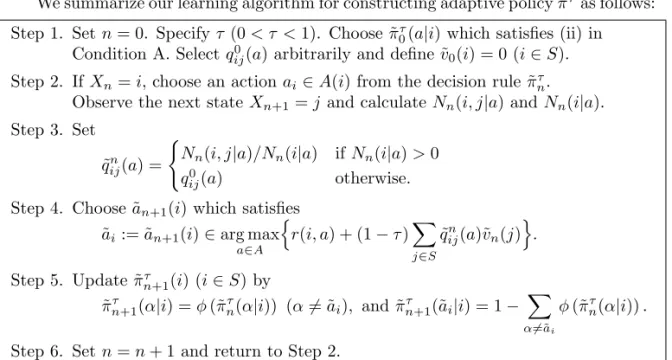
We summarize our learning algorithm for constructing adaptive policy ˜πτas follows:
Step 1. Set n = 0. Specify τ (0 < τ < 1). Choose ˜πτ
0(a|i) which satisfies (ii) in
Condition A. Select q0
ij(a) arbitrarily and define ˜v0(i) = 0 (i∈ S).
Step 2. If Xn= i, choose an action ai∈ A(i) from the decision rule ˜πnτ.
Observe the next state Xn+1= j and calculate Nn(i, j|a) and Nn(i|a).
Step 3. Set ˜
qnij(a) =
{
Nn(i, j|a)/Nn(i|a) if Nn(i|a) > 0 q0
ij(a) otherwise.
Step 4. Choose ˜an+1(i) which satisfies ˜
ai:= ˜an+1(i)∈ arg max a∈A { r(i, a) + (1− τ)∑ j∈S ˜ qnij(a)˜vn(j) } . Step 5. Update ˜πτ n+1(i) (i∈ S) by ˜
πn+1τ (α|i) = ϕ (˜πτn(α|i)) (α ̸= ˜ai), and ˜πn+1τ (˜ai|i) = 1 − ∑ α̸=˜ai
ϕ (˜πnτ(α|i)) .
Step 6. Set n = n + 1 and return to Step 2.
Figure 3.1: Learning Algorithm for vanishing rate τ .
4. A numerical experiment
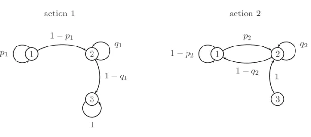
In this section, we give a simulation result for learning algorithm in Section 3. Consider the three state MDPs with S ={1, 2, 3} and A = {1, 2}, whose transition matrices are parameterized with 0 < p1, q1, p2, q2 < 1 and reward function r(i, a) (i∈
S, a∈ A) are given in Table 4.1 and Figure 4.1.
state action parameterized transition matrices reward
i a j = 1 j = 2 j = 3 r(i, a) 1 1 p1 1− p1 0 3 0 2 1− p2 p2 0 2.5 2 1 0 q1 1− q1 2 0 2 1− q2 q2 0 1.5 3 1 0 0 1 1 0 2 0 1 0 0.5
Table 4.1: Data of simulated MDPs.
From this table and figure, we observe that the transition matrix q has a property of communicating provided that 0 < p1, q1, p2, q2 < 1. We denote by ˜ψn the average
1 2 3 1 − p1 p1 q1 1 − q1 1 action 1 1 2 3 p2 1 − p2 q2 1 − q2 1 action 2
Figure 4.1: Transition diagrams parameterized with 0 < p1, q1, p2, q2< 1.
present value until n-th time, which is defined by
˜ ψn = 1 n n∑−1 t=0 r(Xt, ∆t) (n= 1).
To calculate the quantity explicitly, we set ˜πτ
0(·|i) = (12, 1
2) for each i∈ S and q0 with
p1=25, q1= 12, p2=103, q2= 103, i.e., q0= (q0ij(a)) = { (q0ij(1)) = 2 5 3 5 0 0 12 12 0 0 1 , (q0 ij(2)) = 7 10 3 10 0 7 10 3 10 0 0 1 0 }.
We use a strictly increasing function ϕ such that
ϕ(x) =
( xN
1 + xN
)1/N
where N denotes the number of states in S. Let{bn} be such that b0 = 1 and bn = n−1/N(n≥ 1). It is easily checked that the property (i) in Condition A is satisfied with
bn+1= ϕ(bn) (n= 0).
Now, we make numerical experiments with the true transition matrices whose pa-rameters are given by p1= p2= 13, q1= q2= 25, i.e.,
q = (qij(a)) = { (qij(1)) = 1 3 2 3 0 0 25 35 0 0 1 , (qij(2)) = 2 3 1 3 0 3 5 2 5 0 0 1 0 }.
values HHHHH τ n 103 5× 10³ 104 5× 10⁴ 105 106 ˜ ψn 0.5 2.1104 2.1437 2.1569 2.1801 2.1876 2.2002 0.2 2.1214 2.1468 2.1585 2.1805 2.1878 2.2002 0.1 2.1224 2.1470 2.1586 2.1805 2.1878 2.2002 0.01 2.1184 2.1462 2.1581 2.1804 2.1878 2.2002 decision rules HHHH H τ n 103 5× 10³ 104 5× 10⁴ 105 106 ˜ πτn(1|1) 0.5 0.9003 0.9416 0.9536 0.9729 0.9785 0.9900 0.2 0.8980 0.9413 0.9535 0.9728 0.9785 0.9900 0.1 0.8983 0.9413 0.9535 0.9728 0.9785 0.9900 0.01 0.8937 0.9409 0.9533 0.9728 0.9784 0.9900 ˜ πτn(2|2) 0.5 0.8996 0.9415 0.9536 0.9729 0.9785 0.9900 0.2 0.9002 0.9415 0.9536 0.9729 0.9785 0.9900 0.1 0.9002 0.9415 0.9536 0.9729 0.9785 0.9900 0.01 0.9002 0.9415 0.9536 0.9729 0.9785 0.9900 ˜ πτ n(2|3) 0.5 0.9002 0.9415 0.9536 0.9729 0.9785 0.9900 0.2 0.9002 0.9415 0.9536 0.9729 0.9785 0.9900 0.1 0.9002 0.9415 0.9536 0.9729 0.9785 0.9900 0.01 0.9002 0.9415 0.9536 0.9729 0.9785 0.9900 Table 4.2: The simulation value of ˜ψn and ˜πτ
n for each τ = 0.5, 0.2, 0.1, 0.01.
steps of learning algorithm
a v e ra g e p re se n t v a lu e ˜ ψn 0 1/6 1/3 1/2 2/3 5/6 1 ×10⁶ 2.1 2.14 2.18 2.22
Figure 4.2: The trajectories of ˜ψn(τ = 0.01). The dotted line means the optimal value of average reward.
Considering the optimal average reward ψ(q) = 42/19≈ 2.2105 and the q-optimal stationary policy f∗ with f∗(1) = 1, f∗(2) = f∗(3) = 2, it is seen that ˜ψn → ψ(q) =
42/19 and ˜πτ
n(1|1), ˜πτn(2|2), ˜πτn(2|3) → 1 as n → ∞ hold from the above Table 4.2 and
Figure 4.2. The results of the above simulation show that the learning algorithm is practically effective for the communicating class of transition matrices.
References
Bather, J. (1973). Optimal decision procedures for finite Markov chains. II. Communi-cating systems. Adv. in Appl. Probab., 5:521–540.
Bertsekas, D. P. and Tsitsiklis, J. H. (1996). Neuro-Dynamic Programming. Athena Scientific.
Billingsley, P. (1961). Statistical inference for Markov processes. The University of Chicago Press.
Federgruen, A. and Schweitzer, P. J. (1981). Nonstationary Markov decision problems with converging parameters. J. Optim. Theory Appl., 34(2):207–241.
Hern´andez-Lerma, O. (1989). Adaptive Markov control processes. Springer-Verlag. Hern´andez-Lerma, O. and Marcus, S. I. (1985). Adaptive control of discounted Markov
decision chains. J. Optim. Theory Appl., 46(2):227–235.
Kemeny, J. G. and Snell, J. L. (1960). Finite Markov chains. D. Van Nostrand. Kurano, M. (1972). Discrete-time Markovian decision processes with an unknown
pa-rameter. Average return criterion. J. Operations Res. Soc. Japan, 15:67–76.
Kurano, M. (1983). Adaptive policies in Markov decision processes with uncertain tran-sition matrices. J. Inform. Optim. Sci., 4(1):21–40.
Kurano, M. (1987). Learning algorithms for Markov decision processes. J. Appl.
Probab., 24(1):270–276.
Lakshmivarahan, S. (1981). Learning algorithms. Springer-Verlag.
Leizarowitz, A. (2003). An algorithm to identify and compute average optimal policies in multichain Markov decision processes. Math. Oper. Res., 28(3):553–586.
Lo`eve, M. (1963). Probability theory. D. Van Nostrand.
Mandl, P. (1974). Estimation and control in Markov chains. Adv. in Appl. Probab., 6:40– 60.
Martin, J. J. (1967). Bayesian decision problems and Markov chains. John Wiley & Sons Inc.
Meybodi, M. R. and Lakshmivarahan, S. (1982). ε-optimality of a general class of learning algorithms. Inform. Sci., 28(1):1–20.
Puterman, M. L. (1994). Markov decision processes: discrete stochastic dynamic
pro-gramming. John Wiley & Sons Inc.
Ross, S. M. (1970). Applied probability models with optimization applications. Holden-Day.
Schweitzer, P. J. (1968). Perturbation theory and finite Markov chains. J. Appl.
Proba-bility, 5:401–413.
Solan, E. (2003). Continuity of the value of competitive Markov decision processes. J.
Theoret. Probab., 16(4):831–845 (2004).
Sutton, R. S. and Barto, A. G. (1998). Reinforcement Learning: An Introducution.
MIT Press.
Received June 7, 2006 Revised February 25, 2007