Panel Data Research Center at Keio University
DISCUSSION PAPER SERIES
DP2017-003 May, 2017
Changes in Household Income Inequality over the Business Cycle:
Husbands’ Earnings and Wives’ Labor Supply in Japan during the Global Financial Crisis
Yoshio Higuchi*
Kayoko Ishii**
Kazuma Sato***
【Abstract】
This study examines how household income inequality in Japan is impacted by changes in a couple’s income and employment status after economic crises, using the Keio Household Panel Survey (KHPS). Our analysis of the periods before and after the Global Financial Crisis yields three notable findings. First, during the recession, incomes stagnated for households in the middle- and high-income brackets, with many experiencing income declines. Conversely, many low-income households saw incomes increase even during the recession, and the overall income gap may have shrunk. Second, concerning the impact of changes in the husband’s income on the wife’s employment, we show that when the husband’s income declines, the added worker effect is observed. This effect was larger in households whose income was originally low. Third, we calculate the Gini coefficient both by using only the husband’s labor income, and also with the wife’s labor income added. We find that the wife’s labor income reduced household income inequality, in particular for several years following the 2008 recession. In conclusion, when focusing only on married households, income inequality appears to shrink during economic recessions.
* Faculty of Business and Commerce, Keio University
**Faculty of Economics, Keio University
*** Faculty of Political Science and Economics, Takushoku University
Panel Data Research Center at Keio University
Keio University
Changes in Household Income Inequality over the Business Cycle:
Husbands’ Earnings and Wives’ Labor Supply in Japan during the Global
Financial Crisis
*
Yoshio Higuchi
Kayoko Ishii¶¶
Kazuma Sato¶¶¶
Summary
This study examines how household income inequality in Japan is impacted by changes in a couple’s income and employment status after economic crises, using the Keio Household Panel Survey (KHPS). Our analysis of the periods before and after the Global Financial Crisis yields three notable findings. First, during the recession, incomes stagnated for households in the middle- and high-income brackets, with many experiencing income declines. Conversely, many low-income households saw incomes increase even during the recession, and the overall income gap may have shrunk. Second, concerning the impact of changes in the husband’s income on the wife’s employment, we show that when the husband’s income declines, the added worker effect is observed. This effect was larger in households whose income was originally low. Third, we calculate the Gini coefficient both by using only the husband’s labor income, and also with the wife’s labor income added. We find that the wife’s labor income reduced household income inequality, in particular for several years following the 2008 recession. In conclusion, when focusing only on married households, income inequality appears to shrink during economic recessions.
J11 Demographic Trends, Macroeconomic Effects, and Forecasts J30 Wages, Compensation, and Labor Cost General
I31 General Welfare, Well-Being
* In conducting this research I received Keio Household Panel Survey microdata produced by the Panel Data Research Center at Keio University. I would like to take this opportunity to express my appreciation.
¶ Faculty of Business and Commerce, Keio University ¶¶ Faculty of Economics, Keio University
1 Introduction
There has been a great deal of societal concern about income inequality since the lengthy recession that followed the bursting of the asset bubble in Japan. There has been a variety of research from an economics perspective in response, investigating the status of and background to income inequality. To summarize previous research, until the mid-2000s, analysis primarily focused on factors behind income inequality. This revealed the aging population and increase in single-person households as main causes (Ohtake 2005). From the mid-2000s onward, research focused on the question of whether income
inequality was increasing, and found that it was not continuously widening1 (Oshio
2010). For example, Oshio (2010), using the Comprehensive Survey of Living Conditions,
found that the Gini coefficient rose from 1997 until 2000, but that it declined in 2003, and rose again in 2006. The latest data from the Ministry of Health, Labour and
Welfare’s 2014 Survey on the Redistribution of Income, released in September 2016,
showed a slight decline in the Gini coefficient compared with the previous survey from 2011, based on equivalent income following redistribution in 2014. These results suggest that there has not been a continuous increase in income inequality since 2000.
What kinds of factors affect changes in income inequality? There is a variety of conceivable causes. This paper focuses on income inequality among married households of working age, focusing on the impact of economic fluctuations, which may affect household incomes via two pathways. The first is through the income of the head of the household (typically the husband in Japan), the main breadwinner. During an economic recession, the household head’s income declines in many cases. If adjustments during a recession are made via reduced bonuses rather than redundancies and other employment adjustment measures, and there is a large income decline in high-income brackets, where bonuses are a large share of income, this may reduce income inequality. When the economy recovers, job creation, which provides major benefits to the low-income brackets, may indeed contribute to shrinking low-income inequality. However, when those in high-income brackets experience major benefits from rising income, this may work to widen income inequality.
The second pathway is female employment, particularly changes to the wife’s
employment. As pointed out in the Cabinet Office’s 2014 White Paper on Gender
Equality, in Japan an increasing number of males are in non-regular employment, and
average incomes are trending downward, so the wife’s income has come to play an increasingly important role in bolstering household income. If the head of the household’s income declines in an economic recession, the shortfall may be filled by the wife getting a job or working longer hours. If the increased supply of labor from the wife is observed mainly among low household-income brackets, this could be expected to narrow income inequality. Conversely, if additional labor from the wife is supplied mainly in high household-income brackets, this could be expected to widen income inequality. In this manner, changes in female employment due to economic fluctuations, in particular changes in the employment of wives, may also contribute to widening or shrinking income inequality.
The impact of economic fluctuations on income inequality has not been adequately
investigated, nor has the actual situation been clarified2. However, investigating these
issues would demonstrate the mechanism behind changes in income inequality, a matter
of considerable research significance. This paper uses the Keio Household Panel Survey
(KHPS) and focuses on working-age married households to investigate the impact on income inequality of changes in the incomes and employment statuses of husbands and wives due to economic fluctuations, through the following two pathways. The first analyzes the relationship between economic fluctuations and changes in the husband’s income. It investigates how the husband’s income changes by quintile, using the KHPS from 2004 until 2015. It focuses on what sort of impact the recession that followed the Global Financial Crisis in 2008 had on the incomes of married men. The second focuses on the interrelationship between the incomes and employment of married couples. This also uses the KHPS to perform quantitative analysis on changes to the wife’s employment behavior when the husband’s income declines, by income quintile. Further, in order to clarify the impact of the wife’s employment on income inequality, we calculated the Gini coefficient using only the husband’s income and also using the couple’s combined incomes, and then compared them.
In consideration of income inequality, it is important to take into account of single-person, single-mother, and elderly households. However, the main focus of this paper is to analyze the impact on income inequality of the interrelationship between employment and incomes for married couples. Therefore, it restricts analysis to working-age married households. To this end, in the next section, we discuss the significance and issues
2 Although Mori (2002), Hamada (2007), and Urakawa (2007) have investigated the impact of the wife's
involved in setting this restriction. In addition, we assess the impact of the Global Financial Crisis on the labor market, the subject of this analysis. In the third section, we investigate the relationship between economic fluctuations and changes in the husband’s income. In the fourth section, we investigate changes in the wife’s employment behavior when the husband’s income declines. In the fifth section, we examine the impact of the wife’s income on household income inequality.
2 Analysis subjects and characteristics
This section considers the significance of limiting analysis to married working-age households when researching income inequality. It then assesses what sort of impact the Global Financial Crisis had on the labor market, the focus of this analysis.
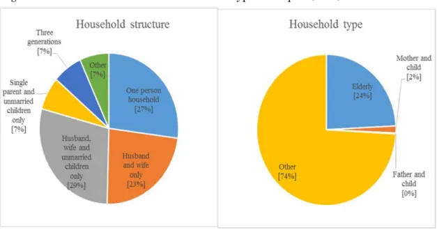
Figure 1: Household structure and household types in Japan (2014)
Source: Prepared by the author based on figures from the Ministry of Health, Labor and Welfare, Comprehensive Survey of Living Conditions 2014.
The subjects of this research are working-age married households—specifically, married households in the KHPS from 2004 until 2015 where the husband is aged
between 20 and 593 in the survey year. Limiting the scope to married households
enabled analysis of not only what sort of impact changes in the household head’s (husband’s) income had on income inequality, but also the impact of changes in the wife’s
employment behavior. In recent years, as employment has become increasingly unstable, the wife’s income has become more important to the household, so it is meaningful to focus on the impact of changes to the husband’s and wife’s combined income on income inequality among households.
However, we should note that limiting the discussion to working-age married households means that households that are at high risk of having low incomes, such as single-person, single-parent and elderly households are excluded from the analysis. Figure 1 shows household structures and household types in Japan from the Ministry of
Health, Labor and Welfare’s Comprehensive Survey of Living Conditions 2014. By
structure, the only households excluded from this analysis are single-person households, which account for 27% of the total, and those with a sole parent and unmarried children,
which account for 7%. By type, elderly households4, which account for 24% of the total,
are excluded from the analysis.
Limiting analysis to working-age5 households, Figure 2 from the KHPS shows where
unmarried households (single-person and single-parent households, which are excluded from this analysis) lie in terms of income distribution. The lower the income bracket, the greater the share of unmarried households. However, it is necessary to point out that unmarried households form a very small proportion of working-age households in Japan.
Incidentally, Figure 3 shows the Gini coefficient6 for all households where the head was
aged 20–59 years, including single-person and single-parent households, calculated using the household head’s income in the KHPS data. In 2003, when the unemployment rate reached 5.3%, near its historical peak, the Gini coefficient was high at 0.325, and subsequently as the unemployment rate dropped, the Gini coefficient also declined, reaching 0.307 in 2008. In 2009, when the unemployment rate jumped to 5.1% due to the Global Financial Crisis, the Gini coefficient rose to 0.314. Subsequently, in line with the falling unemployment rate, the Gini coefficient also fell. In 2013, when the unemployment rate was in the 4.0% range, the Gini coefficient was 0.292. In this manner, income inequality for all working-age households based on the household head’s income behaves in a countercyclical fashion. It is necessary to reiterate that the research results of this paper do not address income inequality for society as a whole. The discussion is limited solely to income inequality among working-age married households.
4 Comprising households of people aged at least 65 years, or that also contain unmarried members under 18. 5 Defined here as households where the head (the husband in a couple) is aged 20–59 years.
6 Due to the nature of panel data, inequality may be in a secular decline, but aggregate results show considerable movement.
Figure 2: Proportion of married and unmarried households by income quintile
Note 1:Estimated by pooling data from the KHPS 2004–2015.
Note 2: Unmarried households are households where the head is not married and aged from 20–59 years, excluding students.
Note 3: Quintiles calculated every year based on labor income of the household head aged 20–59 years (husband in case of married households).
Source: Author’s estimates, based on KHPS 2004–2015
Figure 3: Unemployment rate and time-series estimates of Gini coefficient for all working-age households
Note 1: Gini coefficient calculated using labor income of household head, where the head (husband in case of married households) is aged 20–59 years. Households where the head is a student were excluded from calculations.
Note 2: Sample limited to cases where data on labor income for the next year available, so data are until 2013
0% 20% 40% 60% 80% 100% 1st quintile 2nd quintile 3rd quintile 4th quintile 5th quintile Married Unmarried
(KHPS 2014).
Source: Author’s estimates, based on Ministry of Health, Labour and Welfare Labor Force Survey and KHPS 2004– 2015.
Features of the impact of the GFC, the focus of the analysis, on the labor market are
summarized here7. The GFC was triggered by the collapse of the American investment
bank Lehman Brothers in September 2008. It had a severe impact on Japan’s labor
market. According to the Labor Force Survey from the Ministry of Internal Affairs and
Communications, the number of unemployed men grew by 440,000 from 2008 to 2009, and the number of unemployed women grew by 260,000. The unemployment rate for men rose by 1.2 percentage points, from 4.1% to 5.3%, and that for women rose by 1.0 percentage points, from 3.8% to 4.8%. Since the early 2000s, the number of unemployed people in Japan had been declining, partly due to economic recovery, so the large rise in the number of unemployed people illustrates the severity of the shock.
Also, the same survey showed changes in employment status from 2008 to 2009. Among men, the number of regular employees shrank by 220,000, and the number of non-regular employees shrank by 330,000. Among non-non-regular employees, the biggest decline was for temporary workers, with a fall of 180,000. In contrast, regular female employees grew in number by 70,000, and there was a decline of just 50,000 in the number of non-regular female employees. In the non-non-regular category, the number of female temporary workers declined by 130,000, less than the decline for male workers in this category. For women, the number of contract, short-term contract, and part-time workers rose from 2008 to 2009. This ameliorated the decline in non-regular employees
.
Looking at changes in employee numbers by industry from 2008 to 2009 in the Labor
Force Survey, the number of male employees declined by 570,000 overall8. The decline
was mainly in manufacturing, with about 340,000 fewer employees9. The number of
female workers rose by 10,000. By industry, the number of women in manufacturing fell by 250,000, similar to the number for men, but there was an increase of 170,000 women in the medical and welfare sectors, as well as gains in other service industries, which offset the decline in manufacturing.
7 See Appendices 1-4 for detailed figures regarding impact of global financial crisis on labor market.
8 Changes in employee numbers by industry include changes in the numbers of executives and regular and non-regular employees.
9 Sectors with large drops in employment for males outside the manufacturing sector included construction (120,000) and services not elsewhere classified (140,000)
What sort of relationship was there between unmarried working-age households, which
are excluded from this analysis, and the GFC? According to the Labor Force Survey,
prior to the GFC (in 2007)10, married men accounted for 69% of the total among male
employees overall11 over age 15 years. Only 40% of male temporary workers, for whom
the global financial crisis resulted in the most unemployment, were married. That is, more than half of the male temporary employees, who were greatly affected by the shock of the GFC, were unmarried at the time and so not included in this analysis. Nevertheless, it is important to note that they were strongly affected by the GFC.
To summarize the above results, the number of employees fell sharply during the GFC, with the effects particularly notable among male temporary workers. As pointed out by Nagahama (2012), the background to this was a strong impact from the GFC on the manufacturing sector, where men are heavily employed, due to a slump in global consumption. In contrast, female employment increased in some cases during the GFC, so the impact was the opposite. Female employment patterns and the industries they worked in showed employment growth even during the GFC, so it may have been easier for women to find work during this time.
Finally, we touch upon data used. The KHPS, which provided data used in the analysis in this paper, is a survey conducted in February every year. Questions on income ask about income in the previous year and those on employment status ask about employment status in the previous month (January). As a result, when data from KHPS from 2004 until 2015 are used, information on income covers the period from 2003 until 2014. In this paper, we refer to years according to the year the data are from, not the survey year.
3 Economic fluctuations and changes in husband’s income
The section uses data from KHPS from 2004 to 2015 to investigate the relationship between economic fluctuations and changes in income, limiting analysis to married men. Specifically, we assess changes in husband’s income from the current year (period t) to the next year (period t+1), by husband’s income bracket. We examine the descriptive data to see whether there are differences between developments at the time of the GFC and
10 Refer to Appendix 4.
other periods.
Before discussing analysis, Table 1 shows characteristics of the sample used in analysis
in this section. They cover married men12 aged from 20–59 years for each period t who
were employed in period t. Table 1 shows aggregate values for pooled data from KHPS from 2004 to 2015, by income quintile. The income quintiles were calculated for each year based on the husband’s income from work over the year (before deducting taxes and insurance premiums). The sample contains self-employed respondents, so there is a possibility that business income is included. Looking at husband’s age by income quintile shows that in the fifth quintile, the highest, the husband’s age is greater; in the first, the lowest income quintile, the husband’s age is on average around the middle of the range. The husband’s employment status varies markedly between the lower quintiles and the others. For the lower income brackets, and for the first quintile in particular, the share of regular employment is notably low while that of non-regular employment is high. Furthermore, the share of self-employed and family-business workers is larger than that
in the middle- and high-income brackets13.
Table 1: Characteristics of analysis subjects
Note 1: Pooled data from KHPS from 2004 to 2015.
Note 2: Subjects were married men aged 20–59 years employed during period t. Income brackets aggregated every year based on income (annual income before tax and social security deductions) of married men aged 20-59.
Source: Author’s estimates using KHPS from 2004 to 2015.
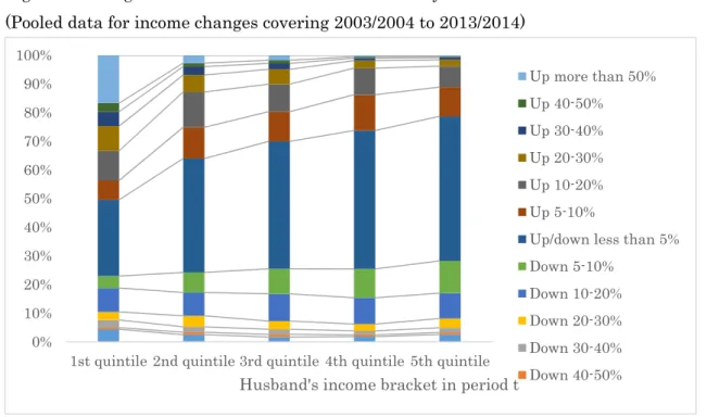
Figure 4 shows to what extent income increased (resp., declined) from period t to period t+1 by husband’s income quintile in period t, using pooled KHPS data from 2004 to 2015. As discussed previously, the KHPS asks about the previous year’s income, so the years shown in the figure do not refer to the survey year but the year in which income was
12 Restricted to cases where the survey subject and partner are in that age range
13 Here we examine to what extent the first income quintile in this section's analysis overlaps with the poor demographic in society overall. Comparing equivalent gross income of the subjects in this section with the relative poverty line (half of the median equivalent disposable income) published by the MHLW’s Comprehensive Survey of Living Conditions, 11.5% of the subjects in the first quintile are classified as poor under the relative poverty concept. The relative poverty line referenced in the Comprehensive Survey of Living Conditions covers 2003 to 2012, the closest corresponding periods to the KHPS survey years.
Regular Non-regular Self-employed Family business worker
1st quintile 2,485 44.9 250 46 19 30 4
2nd quintile 2,704 42.7 414 76 5 17 2
3rd quintile 2,911 43.9 543 82 3 14 1
4th quintile 2,720 46.6 709 91 1 8 0
5th quintile 2,624 49.3 1,049 90 1 9 0
N Husband’s average age
(years)
Husband’s average income (million JPY)
earned. As the figure clearly shows, the lower the income of the married man, the greater proportion of rising incomes the following year. Around half of those in the first quintile experienced income gains of more than 5% the next year (an increase of 120,000 JPY on average), and around 15% experienced income gains of more than 50% (1.25 million JPY on average). Wherever the cutoff point is set, the lower the income in the earlier period, the greater the share of respondents whose income grew in period t+1.
Looking at the share of respondents whose income declined a year later, there is not a great difference among income brackets, with roughly 20–30% of households in each experiencing declines of more than 5% in the husband’s income (120,000 JPY on average for the lowest quintile, and 500,000 JPY for the highest). The proportion of respondents who saw declines of more than 10% (250,000 JPY on average in the lowest quintile and more than 1 million JPY for the highest quintile) were generally higher for the lower income brackets.
Figure 4: Changes in husband’s income from t to t+1 by income classes (Pooled data for income changes covering 2003/2004 to 2013/2014)
Note 1: Estimates using pooled KHPS data from 2004 to 2015.
Note 2: Subjects were married men aged 20–59 years employed during period t. Income brackets aggregated every year based on income (annual income before tax and social security deductions) of married men aged 20–59 years. Source: Author’s estimates using KHPS data from 2004 to 2015.
Figure 4 shows pooled movements in husband’s income over two-year periods from 2003
0% 10% 20% 30% 40% 50% 60% 70% 80% 90% 100%
1st quintile 2nd quintile 3rd quintile 4th quintile 5th quintile
Husband's income bracket in period t
Up more than 50% Up 40-50% Up 30-40% Up 20-30% Up 10-20% Up 5-10%
Up/down less than 5% Down 5-10%
Down 10-20% Down 20-30% Down 30-40% Down 40-50%
to 2014. If these movements are shown as a time series, will there be any differences around the time of the GFC? That is, is it possible to observe an impact of the GFC that varies by income bracket? Figure 5 shows the share of households in which the husband’s income rose more than 10% from period t to period t+1, by husband’s income bracket. As shown in Figure 4, there was a markedly high proportion of income gains in the first quintile, up to 60% in some years, and even in years when the proportion was less, 30% saw income gains of more than 10%. Of particular interest is that in income brackets outside the first quintile, there is a sharp decline in the number of households that experienced income gains of more than 10% during the GFC (2008–2009). However, in the first quintile, this phenomenon was not observed. A similar phenomenon was observed when we changed the cutoff point for income gains from 10% to 5%. That is, the lower the income bracket, the greater the share of households with income gains. Except for the first quintile, there was a large increase in the number of households whose income declined at the time of the GFC.
Figure 5: Share of respondents where husband’s income increased more than 10% from period t to period t+1, by income bracket
Note 1: The values in the figure show a time series of the percentage of households where the husband’s income rose more than 10% from period t to period t+1 by husband’s income bracketin period t.
Note 2: Subjects were married men aged 20-59 employed during period t. Income brackets aggregated every year based on income (annual income before tax and social security deductions) of married men aged 20-59.
Source: Author’s estimates using KHPS from 2004 to 2015
0% 10% 20% 30% 40% 50% 60% 70%
1st quintile 2nd quintile 3rd quintile 4th quintile 5th quintile
Figure 6: Share of respondents where husband’s income declined more than 10% from period t to period t+1, by income bracket
Note 1: The values in the figure show a time series of the percentage of households where the husband’s income declined more than 10% from period t to period t+1 by husband’s income bracketin period t.
Note 2: Subjects were married men aged 20–59 years employed during period t. Income brackets aggregated every year based on income (annual income before tax and social security deductions) of married men aged 20–59 years. Source: Author’s estimates using KHPS data from 2004 to 2015.
Figure 6 shows the share of households where the husband’s income declined more than 10% from period t to period t+1, by income bracket. It is apparent that in each income bracket, a higher proportion of households experienced lower income from 2008 to 2009. While there is not a major difference among the income brackets in the share of households where income declined more than 10%, if the cutoff point is set at a relatively small income drop of 5%, the lower the income bracket, the smaller the shock. Surprisingly, incomes in the middle- and high-income brackets were particularly stagnant during the GFC, and not just low-income brackets but medium- and high-income brackets were subject to the shock of lower high-incomes, suggesting that the GFC may have reduced income inequality.
As a check, we review data on why married working males experienced a decline in income. Figure 7 shows the share of respondents who lost or changed jobs by income bracket among respondents who experienced income declines of more than 10%. On the left side, it shows the aggregate results pooled from 2003 to 2014. On the right side, it
0% 10% 20% 30% 40%
1st quintile 2nd quintile 3rd quintile 4th quintile 5th quintile
shows aggregates for the GFC period alone. Married males in the first quintile were most likely to experience job loss: around 10% over the entire time frame and 20% at the time of the GFC. There is also a difference among income brackets regarding changing jobs. Similarly, a greater proportion of those in the lower-income brackets tend to change jobs. In the lower-income bracket, job loss or changing jobs is one factor in income decline, but it is not the primary cause.
Figure 7: Proportion who lost or changed jobs among those whose income declined by more than 10% from period t to period t+1 (by husband’s income bracket)
Note 1: Subjects were married men aged 20–59 years employed during period t, whose income declined more than 10% from period t to period t+1. Income brackets aggregated every year based on income (annual income before tax and social security deductions) of married men aged 20-59.
Source: Author’s estimates using KHPS from 2004 to 2015.
What then, is the cause of income decline among high-income brackets? Figure 8 shows aggregate figures on whether respondents who experienced income declines of more than 10% while continuing employment at the same company experienced decreased bonuses. Similar to before, the left-hand side shows aggregate data pooled for 2003 through 2014, while the right-hand side shows aggregate data for the time of the GFC alone. This shows that the higher the income bracket, the greater the proportion of respondents who experienced decreased bonuses. Further, this proportion is particularly large at the time
of the GFC14.
14 In the low-income brackets, there are more workers in non-regular employment and other formats with no
0% 10% 20% 30% 40% 50% 60% 70% 80% 90% 100% Changed job Lost job Continued employment 0% 10% 20% 30% 40% 50% 60% 70% 80% 90% 100% Changed job Lost job Continued employment
Figure 8: Share of employees who experienced decreased bonuses while continuing employment at the same company among employees whose income fell more than 10% from period t to period t+1
Note 1: Subjects were married men aged 20–59 years employed during period t, whose income declined more than 10% from period t to period t+1. Income brackets aggregated every year based on income (annual income before tax and social security deductions) of married men aged 20–59 years.
Source: Author’s estimates using KHPS data from 2004 to 2015.
From the above results, the following two points are clear. First, incomes stagnate for middle- and high-income brackets in particular when there is a major economic recession. Also, not just low-income brackets, but middle- and high-income brackets experience the risk of decreasing incomes, so the GFC may have reduced income inequality. The second point is that in a recession, while there is a higher risk of job loss or unemployment for lower-income brackets, other changes, such as adjustments via bonuses and other wage measures, are common, particularly for high-income brackets. It is not the case that during recessions, only low-income brackets experience damage from unemployment. No matter what the bracket, there are widespread declines in income, suggesting this may also reduce income inequality during recessions.
4 Relationship between decline in husband’s income and changes in wife’s employment
bonuses than in other income brackets.
0% 10% 20% 30% 40% 50% 60% 70% 80% 90% 100%
Bonus not cut Bonus cut
0% 10% 20% 30% 40% 50% 60% 70% 80% 90% 100%
This section focuses on the impact of changes in the husband’s income, declines in particular, on the wife’s employment status. When the husband’s income declines due to an economic recession or unemployment, it is possible that a working wife will increase her overtime hours or one who has not been in the workforce will start working, thus increasing the supply of labor, in order to maintain a certain living standard. This is
called the “added worker effect”15 (Higuchi 2001). This added worker effect is thought to
be related to household income inequality. Specifically, when a household’s income level is originally high, the impact of lowered income from the husband is negligible, and the added worker effect from the wife is also small. However, if the household income is low to start with, the impact of a decline in the husband’s income is severe, so the added worker effect from the wife is expected to be larger. As such, even if the husband’s income declines, it is possible that there will be a strong added worker effect among brackets with low household-income levels, which will work to suppress the expansion of household income inequality. This section examines the mechanisms by which the wife’s employment reduces household income inequality. The data used are from the KHPS from 2004 to 2015. The subjects are married couples where the husband is younger than 60 years.
4.1 Estimation methodology
We estimate three models to analyze the added worker effect attributable to the wife. The first analyzes whether a wife who had withdrawn from the labor market re-enters due to a decline in the husband’s income. The second examines whether a working wife continues to work at her current job due to a decline in the husband’s income. The third analyzes whether a working wife increases her employment hours due to a decline in the husband’s income.
The discussion below starts with the first estimated model. Analysis of the wife re-entering the labor market uses the logit model below.
15 There has been a great deal of research into the added worker effect in Japan and abroad. Much non-Japanese
research points to the existence of the added worker effect (Heckman and MaCurdy 1980, 1982; Lundberg 1985; Stephens 2002; Skoufias and Parker 2006). One representative study is by Stephens (2002). It analyzes the wife's labor supply before and after the husband's unemployment. This showed that the wife's added worker effect is not apparent just at the time of the husband's unemployment, but subsequently as well. Much Japanese research points out the presence of the added worker effect, similar to outside Japan (Higuchi and Abe 1999, Kuroda and Yamamoto 2007; Kohara 2007; Kohara 2010; and Sato 2012). One representative study by Kohara (2007) analyzes the impact of the husband's unemployment on the wife's labor supply. This shows that the husband's
unemployment increases the wife's working hours and that the fewer financial assets in a household, the larger the impact.
∗ ∙ (1) is a dummy variable that takes a value of 1 when the wife changes her status to employed or looking for work from not in the labor force, and 0 if she remains out of the
labor force. is a vector of individual attributes, including educational history
dummies for the husband and wife, wife’s age, a dummy for presence of a child under three years old, number of children, savings (in millions of JPY 10,000, debts (in millions
of JPY), job-offers-to-applicants ratio by prefecture, and a year dummy. is a dummy
variable that takes a value of 1 when the husband’s income declines more than 10% from
period t-1 to period t and 0 otherwise. is a household income quintile dummy, and
indicates equivalent household income at period t-1. In this analysis we prepared by quintile dummies (for the first, second, third, fourth, and fifth quintiles). The first quintile dummy (for the lowest household income quintile) and the fifth quintile dummy (for the highest household income quintile) were used as explanatory variables.
Reference group are second, third, and fourth quantiles. ∙ is the cross term
between whether the husband’s income declines more than 10% dummy and the household-income fifth-quintile dummy. are unobservable fixed effects and
indicates error terms.
Of these variables, those of most interest in this analysis are the estimation results for
the cross term ∙ for the husband’s income declines more than 10% dummy and
the household-income fifth-quintile dummy. This cross term shows for which household income brackets the impact of declining husband’s income is greatest. If the sign is positive, the wife’s added worker effect is stimulated; if negative or found to be insignificant, it means there is no added worker effect from the wife. We examine this
using pooled logit and random effect logit models16. In the estimates, we incorporated
analysis using the cross term for the job-offers-to-applicants ratio by prefecture and the year-ago household-income dummy as an additional independent variable to investigate whether changed labor market supply-and-demand conditions affect the wife’s re-entering the workforce.
The second analysis regarding continued employment is estimated using the logit model below.
∗ ∙ (2)
16 We investigated using a fixed-effect model, but there was not enough variation in the dependent variable, making it impossible to obtain estimates, so we abandoned this approach.
The dependent variable is a dummy variable set to 1 if a wife who was working at period t-1 continued working at the same company at period t and 0 if not. This analysis applies to only employed workers. Just as in Formula (1), it uses ( ) for individual
attributes and a dummy for when the husband’s income declines by more than 10% ( ).
Whereas Formula (1) used a dummy for household income at t-1, Formula (2) uses ( )
as a dummy for husband’s income quintile at period t-1. This is because in the case of a working wife, her labor income is reflected in household income at period t-1, becoming an endogenous variable and potentially causing a bias in the estimation results. The use of a dummy for the husband’s income quintile deals with this bias. Formula (2) uses the
cross term ( ∙ ) for the dummy of whether husband’s income declines by more than
10% against husband’s income quintile dummy, and we focus on the estimation results. Estimations are made using the pooled logit and random-effect logit models.
Third, analysis regarding an increase in the wife’s working hours is estimated using ordinary-least-squares minimization in the model below.
∆ ∙ (3)
∆ is the difference in the wife’s weekly working hours between period t-1 and period
t. The analysis covered only workers with jobs and the explanatory variables include a regular employment dummy added to Formula (3). Note that the estimates use pooled OLS, fixed-effect OLS, and random-effect OLS.
Using the above estimation methodology, we investigated the impact of a decline in husband’s income on wife’s employment behavior. An examination of previous research, including that by Kuroda and Yamamoto (2007) and Kohara (2010), shows that the wife’s added worker effect primarily takes the form of an unemployed wife entering the workforce (by a wide margin). In this research as well, we focus on whether similar trends are apparent. Basic statistics regarding the variables used in the estimations are shown in Table 2.
Source: Author’s estimates using KHPS data from 2004 to 2015.
4.2 Estimation results
Table 3 shows the results of investigating the impact of the decline in husband’s income on wife’s entry into the labor market. (A1) and (A3) in the table are pooled logit estimation results, and (A2) and (A4) are estimation results from the random-effect logit model. The values in the table are marginal effects.
Looking at the husband’s income decline dummy and year-ago household income dummy cross terms for (A1) and (A2) shows that, in both cases, the cross terms for the decline of 10% or more dummy and first-quintile household income dummy are significant and positive. This result means that when the husband’s income declines, the percentage of wives newly entering the labor market in the low household-income bracket increases. In contrast, the cross term for the husband’s income declines more than 10% dummy and the fifth-quintile household income dummy was not significant. This means that even if the husband’s income declines by more than 10%, in households that were originally in a high-income bracket, there is no impact on the wife’s employment behavior. The above results mean that the lower the household’s household income level, the more sensitive to a decline in husband’s income, and the more labor supply is increased. Because the added worker effect from the wife is present, there is a possibility that the wife’s employment suppresses the widening of income inequality Average Standard deviation Average Standard deviation Average Standard deviation
Wife’s new employment dummy 0.13 0.34
Wife’s continued employment dummy 0.95 0.21
Difference in wife’s weekly work hours 0.51 15.02
Husband’s income declined more than 10% dummy 0.15 0.36 0.18 0.38 0.17 0.38
Year-ago household-income quintile 5th quintile 0.15 0.36 2nd-4th quintile 0.61 0.49
1st quintile 0.24 0.43
Year-ago husband’s income quintile 5th quintile 0.19 0.39 0.19 0.39
2nd-4th quintile 0.62 0.49 0.62 0.48
1st quintile 0.19 0.39 0.19 0.39
Job-offers-to-applicants ratio by prefecture 0.87 0.33 0.89 0.34 0.89 0.35
Husband’s education dummy Junior/senior high 0.44 0.50 0.54 0.50 0.53 0.50
Technical/junior c 0.06 0.24 0.07 0.26 0.08 0.27
University gradua 0.45 0.50 0.34 0.47 0.34 0.47
Wife’s education dummy Junior/senior high 0.45 0.50 0.50 0.50 0.50 0.50
Technical/junior c 0.32 0.47 0.29 0.45 0.29 0.45
University gradua 0.16 0.37 0.13 0.34 0.13 0.34
Wife’s age 42.47 8.36 45.12 7.29 44.75 7.28
Wife’s employment status dummy Regular employment 0.28 0.45
Non-regular employment 0.72 0.45
Child under three dummy 0.23 0.42 0.05 0.22 0.06 0.24
Number of children 1.83 0.98 1.88 0.92 1.88 0.92
Savings millions of JPY 6.42 10.93 5.26 8.45 5.07 8.23
Debt millions of JPY 8.63 11.73 8.17 11.95 8.17 11.78
Variable
Analysis of wife’s new employment
Analysis of wife’s continued employment
Analysis of changes to wife’s work hours
among households17.
In other variables, the coefficient for the job-offers-to-applicants ratio by prefecture, which shows changes to supply-and-demand conditions in the labor market due to economic fluctuations, shows positive and significant results for (A1) and (A2). These results mean that new employment by the wife increases when the job-offers-to-applicants ratio rises in an economic recovery. Further, these results may also show that new job creation is suppressed during an economic downturn and there is a discouraged worker effect, whereby an increasing number of wives remain outside the labor force. If the discouraged worker effect has a different impact on different household income brackets, the impact of the added worker effect on reducing household income inequality may vary. In order to assess this point, we conducted estimations with the addition of cross terms between the job-offers-to-applicants ratio by prefecture and year-ago household income dummy in (A3) and (A4). The results (A3) and (A4) showed that cross terms between the job-offers-to-applicants ratio by prefecture and year-ago household income dummy were not significant. This implied that there were no variations in the impact of the discouraged worker effect among different household income brackets.
Table 3: Impact of decline in husband’s income on wife’s entry into labor market
17 This research focuses on households where there is an unemployed wife during recessions, but it is possible that there are households in which a wife who had already been working loses income due to a recession. In this case, particularly in low-income households, if the wife loses her job and the household faces a decline in income, an economic recession will not necessarily reduce household income inequality. In order to assess this, we carried out logit analysis using an unemployment dummy a dependent variable with a value of 1 when the working wife lost her job and 0 when she continued working. This analysis focused on the cross terms of the job-offers-to-applicants ratio by prefecture and year ago household income dummy. The analysis showed that neither of the cross terms for the job-offers-to-applicants ratio by prefecture or year ago household income dummy was significant. This means that wives in low-income households do not necessarily lose their jobs and face a decline in income.
Note 1: ***, **, and * indicate that the respective estimated coefficients are significant at the 1%, 5% and 10% levels. Note 2: Figures in parentheses ( ) are standard errors robust to non-uniform distribution.
Note 3: Table figures show marginal effects.
Note 4: In the estimates, educational history dummies for the husband and wife, wife’s age, number of children, savings in millions of JPY, debts in millions of JPY, and a year dummy are used as explanatory variables.
Source: Author’s estimates using KHPS from 2004 to 2015.
Table 4 shows the results of investigating the impact of a decline in husband’s income on wife’s continued employment. Among the estimation results, looking at the cross terms between the dummy for decline in husband’s income and husband’s year-ago income quintile dummy, no cross terms were significant. These results mean that even if income levels were different, there was no difference in the probability that the wife would continue working due to a decline in husband’s income. We considered that there may be a higher probability of the wife remaining employed if a decline in the husband’s income prevented her from leaving her job, but we found no impact on this from changes in the
husband’s income18.
Table 4: Impact of decline in husband’s income on wife’s continued employment
18 We also conducted analysis dividing wife's employment status one year prior into regular and non-regular employment, but the cross terms with the husband's income decline dummy and year-ago household income dummy were not significant. Further, we also conducted analysis taking into consideration not just the wife leaving employment, but whether or not she changed jobs, but none of the cross terms was significant.
(A1) (A2) (A3) (A4)
Husband’s income declined more than 10% dummy -0.018 -0.027 -0.018 -0.027 (0.022) (0.023) (0.022) (0.023) Year-ago household-income quintile dumm5th quintile -0.034 -0.026 -0.076 -0.034
ref: 2nd-4th quintile (0.025) (0.029) (0.058) (0.062)
1st quintile 0.019 0.025 -0.004 0.013 (0.016) (0.019) (0.038) (0.043) Year-ago household-income quintile dumm5th quintile 0.043 0.044 0.042 0.044 Husband’s income declined more than 10% dummy (0.057) (0.054) (0.057) (0.054)
1st quintile 0.059* 0.064* 0.061* 0.065* (0.034) (0.038) (0.035) (0.038) Job-offers-to-applicants ratio by prefecture 0.094*** 0.093*** 0.083*** 0.088**
(0.025) (0.032) (0.028) (0.035) Year-ago household-income quintile dumm5th quintile 0.046 0.009 Job-offers-to-applicants ratio by prefecture (0.058) (0.057)
1st quintile 0.025 0.013
(0.039) (0.043) Estimation methodology Pooled Probit RE Probit Pooled Probit RE Probit
Log-likelihood -1166.851 -1144.097 -1166.424 -1144.053
Sample size 3,185 3,185 3,185 3,185
Note 1: ***, **, and * indicate that the respective estimated coefficients are significant at the 1%, 5% and 10% levels. Note 2: Figures in parentheses ( ) are standard errors robust to non-uniform distribution.
Note 3: Table figures show marginal effects.
Note 4: In the estimates, educational history dummies for the husband and wife, wife’s age, number of children, savings in millions of JPY, debts in millions of JPY, and a year dummy are used as explanatory variables.
Source: Author’s estimates using KHPS data from 2004 to 2015
Table 5 shows the results of investigating the impact of a decline in husband’s income on wife’s work hours. Looking at the cross terms for (C3) husband’s income decline dummy adopted using the Hausman test and husband’s year-ago income quintile dummy, none of the cross terms was significant. This means that even at different income levels, there is no impact on the wife’s working hours from a decline in the husband’s income. Just as in previous research by Kuroda and Yamamoto (2007) and Kohara (2010), there is no observable added worker effect from changes in the working wife’s work hours. Table 5: Impact of decline in husband’s income on working wife’s work hours
(B1) (B2)
Husband’s income declined more than 10% dummy -0.011 -0.284
(0.009) (0.222)
Year-ago husband’s income quintile dumm5th quintile -0.013* -0.357
ref: 2nd-4th quintile (0.008) (0.220)
1st quintile -0.003 -0.082
(0.008) (0.219)
Year-ago husband’s income quintile dumm5th quintile -0.006 -0.118
Husband’s income declined more than 10% dummy (0.017) (0.410)
1st quintile 0.006 0.221
(0.017) (0.435)
Job-offers-to-applicants ratio by prefecture 0.000 0.022
(0.010) (0.288)
Estimation methodology Pooled Probit RE Probit
Log-likelihood -1073.519 -1065.804
Sample size 5,926 5,926
Note 1: ***, **, and * indicate that the respective estimated coefficients are significant at the 1%, 5% and 10% levels. Note 2: Figures in parentheses ( ) are standard errors.
Note 3: In the estimates, educational history dummies for the husband and wife, wife’s age, a dummy for wife’s regular employment, number of children, savings (JPY10,000)/100, debts (JPY10,000)/100, and a year dummy are used as explanatory variables.
Source: Author’s estimates using KHPS data from 2004 to 2015.
Summarizing the above results, two points have become clear. First, when the husband’s income declines, there is an added worker effect observed, whereby a wife who had not been previously working supplies additional labor. This effect was observed mainly in households that originally had low incomes. Because the added worker effect is stronger in the lower income households, it is possible that the wife’s employment helps to constrain the expansion of household income inequality when the husband’s income declines. The second point is that when the husband’s income declines there is
no observable change in the supply of labor from working wives19.
5 Impact of wife’s income on household income inequality
Regarding income inequalities in society as a whole, publications from the Ministry of
Health, Labor and Welfare (Survey on the Redistribution of Income) and Ministry of
Internal Affairs and Communications (Comprehensive Survey of Living Conditions) both
show that from the late 2000s through the 2010s, the representative indicator of income
19 In Table 4 and Table 5, we added cross terms for the job-offers-to-applicants ratio by prefecture and husband's year-ago income quintile dummy to analyze the impact of economic fluctuations on working hours and continued employment, but virtually all of the cross terms were insignificant. This result suggests that even if there are differences in the husband's income, economic fluctuations do not result in changes to the wife's working hours or continued employment.
(C1) (C2) (C3)
Husband’s income declined more than 10% dummy 0.385 0.513 0.385 (0.676) (0.860) (0.676) Year-ago husband’s income quintile dummy 5th quintile 0.514 0.160 0.514
ref: 2nd-4th quintile (0.606) (1.332) (0.606)
1st quintile -0.706 -0.554 -0.706 (0.595) (1.161) (0.595) Year-ago husband’s income quintile dummy x 5th quintile -0.724 -0.959 -0.724 Husband’s income declined more than 10% dummy (1.418) (1.850) (1.418)
1st quintile 0.607 0.905 0.607 (1.328) (1.632) (1.328) Job-offers-to-applicants ratio by prefecture 0.411 1.457 0.411
(0.823) (2.106) (0.823)
Estimation method Pooled OLS FE OLS RE OLS
Hausman test
R2 0.004 0.004 0.004
Sample size 5,742 5,742 5,742
Explanatory variables
inequality, the Gini coefficient, was declining20. It is impossible to grasp yearly
fluctuations in the Gini coefficient or the impact of income source on the Gini coefficient from official published statistics. Therefore, in this section, we look at a time series of the Gini coefficient estimated using only the husband’s income, versus one that includes the wife’s income as well, to see the impact of wife’s income on reducing household income inequality21.
Figure 9 shows the time series for the Gini coefficient calculated using only the husband’s income from work and that using the husband’s and wife’s combined income from work. From the figure, it is clear that the wife’s income has a leveling effect on
household income inequality. There is a secular downtrend in the Gini coefficient22. The
most salient feature is that there is a watershed around the GFC in 2008 and subsequently until 2011: there is a major impact on lessening the Gini coefficient due to the wife’s income. As shown in the previous section, in particular for low-income brackets, disparities among households improved as wives began to work to compensate a decline in the husband’s income due to the GFC.
Figure 9: Gini coefficient calculated using only husband’s income and including wife’s income
20 According to the Ministry of Health, Labour and Welfare’s Survey on the Redistribution of Income, the Gini coefficient measured using equivalent disposable income was 0.322 in 2004 (from survey year 2005, here and after), 0.327 in 2007, 0.322 in 2010, and 0.316 in 2013. According to the Ministry of Internal Affairs and Communications’ Comprehensive Survey of Living Conditions, the Gini coefficient measured using equivalent disposable income was 0.278 in 2004, 0.283 in 2009, and 0.281 in 2014.
21 In Europe and the US there is much reported research into what sort of impact the wife's income has on household income inequality against the backdrop of rising wives’ employment. Researchers have come to different conclusions. Lerman and Yitzhaki (1985) analyze the Gini coefficient in the US and report that since 1979, female incomes have widened household income inequality. Using the same methodology, Urakawa comments that from the early 1990s to the beginning of the 2000s in Japan, the wife's income has contributed to widening the household income inequality in working-age households. Conversely, Harkness, Machin and Waldfogel (1997) and Cancinan and Reed (1999) conclude from their analysis that wives’ income reduces household income inequality or, if it does widen it, the impact is negligible.
22 Changes in the Gini coefficient time series may be affected by problems such as sample dropouts in the panel data and aging of the sample.
Note 1: Analysis subjects are the same as used in the analysis in Section 3, married males aged 20–59 years in employment in period t for whom information was available through period t+1, so aggregate results are until 2013. Income (before deducting tax and social security payments) for husband and wife obtained through their respective work over the period of a year was used for income.
Source: Author’s estimates using KHPS data from 2004 to 2015.
6 Conclusions
This study examines how household income inequality in Japan is impacted by changes in a couple’s income and employment status after economic crises, using the Keio Household Panel Survey (KHPS). Our analysis of the periods before and after the Global Financial Crisis yields three notable findings. First, during the recession, incomes stagnated for households in the middle- and high-income brackets, with many experiencing income declines, typically bonus declines. Conversely, many low-income households saw incomes increase even during the recession, and this suggests that during economic downturns, income inequality between low-income and high-brackets shrinks. Second, concerning the impact of changes in the husband’s income on the wife’s employment, we show that when the husband’s income declines, the added worker effect is observed. This effect was larger in households whose income was originally low. Third, we calculate the Gini coefficient both by using only the husband’s labor income, and also with the wife’s labor income added. We find that the wife’s labor income reduced household income inequality, in particular for several years following the 2008 recession.
To summarize the above, when focusing only on married households, income inequality appears to shrink during economic recessions. The background to this is income declines by the husband in medium- and high-income brackets and assumption of work by wives in low-income brackets. These results show that a couple’s employment and income affect income inequality at times of economic fluctuation, a new finding not pointed out in previous research.
We showed that the Gini coefficient for all households by considering household head’s income, including that of unmarried households (single-person and single-parent households) shows countercyclical movements. During economic recoveries, income inequality shrinks. When the economy worsens, inequality expands. Single-person and single-parent households suffer a strong impact from increased unemployment when the economy worsens, but the effect is smaller on household heads in married households, and indeed there is a strong impact from bonuses and overtime pay. Furthermore, in addition, increased employment opportunities for women encourage wives to start working, particularly in low-income households, increasing income and reducing income inequality during recessions. In the future, it will be necessary to ascertain whether these developments are specific to the Global Financial Crisis, or whether they may be observed as general trends during other processes in the economic cycle. It is nonetheless undeniable that changes in labor supply by household and attribute have a major impact on household income inequality.
Appendix 1 Number of unemployed persons and changes in unemployment rate by gender
Source: Labor Force Survey, Statistics Bureau, Ministry of Internal Affairs and Communications Numbers
(10,000 persons)
Year-on-year
change Unemployment rate
Year-on-year change Numbers (10,000 persons) Year-on-year
change Unemployment rate
Year-on-year change 2002 219 5.5 140 5.1 2003 215 -4 5.5 0 135 -5 4.9 -0.2 2004 192 -23 4.9 -0.6 121 -14 4.4 -0.5 2005 178 -14 4.6 -0.3 116 -5 4.2 -0.2 2006 168 -10 4.3 -0.3 107 -9 3.9 -0.3 2007 154 -14 3.9 -0.4 104 -3 3.7 -0.2 2008 159 5 4.1 0.2 107 3 3.8 0.1 2009 203 44 5.3 1.2 133 26 4.8 1 2010 207 4 5.4 0.1 127 -6 4.6 -0.2 2011 187 -20 4.9 -0.5 115 -12 4.2 -0.4 2012 173 -14 4.6 -0.3 112 -3 4 -0.2 2013 162 -11 4.3 -0.3 103 -9 3.7 -0.3 2014 141 -21 3.7 -0.6 95 -8 3.4 -0.3 2015 134 -7 3.6 -0.1 88 -7 3.1 -0.3
Appendix 2 Number of workers by employment status and gender
Source: Labor Force Survey, Statistics Bureau, Ministry of Internal Affairs and Communications
Appendix 3 Number of male and female employees by industry
Source: Labor Force Survey, Statistics Bureau, Ministry of Internal Affairs and Communications
Appendix 4 Marital status of male employees over 15-years-old by employment status
(A) males (10,000 persons)
Part-time worker Temporary worker 2002 3165 2867 2437 431 229 63 166 10 70 2003 3152 2853 2410 444 235 63 171 13 71 2004 3152 2851 2385 466 236 70 166 28 66 2005 3165 2864 2357 507 247 77 171 42 69 2006 3194 2897 2378 519 247 79 168 49 71 2007 3240 2947 2408 539 255 83 172 54 69 2008 3220 2928 2367 560 248 82 166 55 77 2009 3162 2874 2345 527 250 84 166 37 67 2010 3148 2865 2324 540 259 87 172 35 66 2011 3163 2885 2313 571 276 94 182 39 62 2012 3147 2865 2300 566 272 97 175 36 61 2013 3140 2878 2267 610 301 101 200 48 147 72 42 2014 3151 2889 2259 630 304 103 201 48 159 76 43 2015 3158 2896 2261 634 312 108 204 50 154 75 42 Change from 2008 to 2009 -58 -54 -22 -33 2 2 0 -18 -10 (B) females (10,000 persons) Part-time worker Temporary worker 2002 2172 2073 1052 1021 825 655 170 33 55 2003 2191 2095 1034 1061 855 685 170 37 58 2004 2220 2124 1025 1098 860 693 166 57 62 2005 2243 2144 1018 1126 872 703 169 64 60 2006 2292 2195 1036 1159 878 713 165 78 70 2007 2332 2237 1041 1196 911 741 170 81 68 2008 2337 2248 1043 1205 906 741 165 85 71 2009 2341 2250 1050 1200 906 733 173 72 73 2010 2361 2273 1051 1223 937 764 172 62 73 2011 2369 2279 1039 1241 954 779 173 59 66 2012 2375 2288 1041 1247 969 792 177 55 67 2013 2405 2323 1027 1296 1019 826 192 68 126 43 40 2014 2436 2351 1019 1332 1042 840 202 71 133 44 42 2015 2473 2388 1042 1345 1053 852 201 76 133 43 41 Change from 2008 to 2009 4 2 7 -5 0 -8 8 -13 2 152 163 157 7 119 130 133 137 142 149 111 181 197 197 -6 Contract employee Entrusted employee 108 Employees Employees excluding executives Regular employee Non-regular employee Other 122 Part-time/tempora ry worker 136 149 151 162 180 174 Dispatched worker from temporary labor agency Other 125 Part-time/tempora ry worker Dispatched worker from temporary labor agency Contract employee Entrusted employee Employees Employees excluding executives Regular employee Non-regular employee
(A) males (10,000 persons)
Total culture and forgricultural industries Fisheries Mining and
quarrying of stone and gravel Construction Manufacturi ng Electricity, gas, heat supply and water Information and communicati ons Transport and postal activities Wholesale and retail trade Finance and insurance Real estate and goods rental and leasing Scientific research, professional and technical services Accommodat ions, eating and drinking services Living related and personal services and amusement services Education, learning support Medical, health care and welfare Compound services Services, not elsewhere classified Government, except elsewhere classified 2008 3226 25 3201 6 2 372 760 29 137 268 470 76 63 97 113 73 123 123 34 255 173 2009 3169 27 3142 5 3 360 726 31 140 272 462 77 62 97 114 74 124 129 31 241 172 Change from 2008 to 2009 -57 2 -59 -1 1 -12 -34 2 3 4 -8 1 -1 0 1 1 1 6 -3 -14 -1 (B) females (10,000 persons)
Total culture and forgricultural industries Fisheries Mining and
quarrying of stone and gravel Construction Manufacturi ng Electricity, gas, heat supply and water Information and communicati ons Transport and postal activities Wholesale and retail trade Finance and insurance Real estate and goods rental and leasing Scientific research, professional and technical services Accommodat ions, eating and drinking services Living related and personal services and amusement services Education, learning support Medical, health care and welfare Compound services Services, not elsewhere classified Government, except elsewhere classified 2008 2320 21 2298 2 0 67 324 3 45 60 474 82 35 53 187 105 136 444 22 188 51 2009 2321 24 2297 3 0 66 299 4 46 63 476 84 35 51 193 109 138 461 20 180 52 Change from 2008 to 2009 1 3 -1 1 0 -1 -25 1 1 3 2 2 0 -2 6 4 2 17 -2 -8 2
(2007 average)
Source: Labor Force Survey, Statistics Bureau, Ministry of Internal Affairs and Communications
Never
married Married Widowed or divorced
Total employees 27% 69% 4% Agriculture 12% 82% 6% Non-agriculture 27% 69% 4% Self-employed 12% 82% 6% Piece worker 0% 100% 0% Family worker 52% 43% 4% Employee 29% 67% 4% Executive 7% 90% 4% Regular employee 28% 68% 3% Part-time/temporary worker 58% 37% 5%
Dispatched worker from temporary labor
agency 55% 40% 6%
Contract/entrusted employee 26% 68% 6%
References
Cancian, M. and Reed, D. (1998), “Assessing the effects of wives’ earnings on family income inequality,” The Riview of Economics and Statistics, 80(1):73‒79. Cancian, M. and Reed, D. (1999), “The impact of wives’ earnings on income inequality:
Issues and estimates,” Demography, 36(2):173-184.
Esping-Andersen, G. (2007), “Sociological explanations of changing income distribution,” American Behavioral Scientist, 50(5):639-58.
Hamada, K. (2007), “Contribution of the Wife’s Income to Couples’ Household Income Inequality,” The Japan Society of Household Economics, 25: pp. 93-104.
Harkness, S. (2010), “The contribution of women’s employment and earnings to household income inequality: A cross-country analysis,” LIS???
Harkness, S. (2010), “Women’s employment and household income inequality,” in Income
and Inequality: Economic disparities and the middle class in affluent countries,
edited by Gornick,J.C. and Jantti, M. Stanford, California: Stanford University Press.
Harkness, S., Machin, S. and Waldfogel, J. (1997), “Evaluating the pin money hypothesis: The relationship between women’s labour market activity, family income and poverty in Britain,” Journal of Population Economics, 10:137-58.
Harkness, S. and Evans, M. (2011), “The employment effects of recession on couples in the UK: women’s and household employment prospects and partners’ job loss,” Journal of Social Policy, 40(4):675-93.
Heckman, J J. and MaCurdy, T. E. (1980)"A Life Cycle Model of Female Labour Supply," Review of Economic Studies, 47(1), pp. 47-74.
Heckman, J J., and MaCurdy, T. E. (1982)"Corrigendum on a Life Cycle Model of Female Labour Supply," Review of Economic Studies, 49, pp. 659-60.
Higuchi, Y., and Abe, M. (1999), “Economic Fluctuations and Analysis of Fixed and Variable Factors in the Timing Of Women’s Marriage, Childbirth and
Employment,” in Modern Women’s Marriage, Childbirth, Employment,
Consumption and Savings as Seen in Panel Data, edited by Higuchi, Y. and Iwata, M., Toyo Keizai Inc., pp. 25-65
Higuchi, Y. (2001), “Economics of Employment and Unemployment,” Nihon Keizai Shimbun-sha
Higuchi, Y., Ishii, K. and Sato, K. (2015), “Income inequality and income change in Japan: dynamic approach through international comparison and time series comparison,” Mita Business Review, 59 (3)
Ishii, K. and Higuchi, Y. (2015), “Rising Non-Regular Employment and Income Inequality: Individuals and Households in Income Inequality–Japan’s Characteristics as Revealed by International Comparisons,” Mita Business Review, 58 (3), pp. 37-55.
Jenkins, S. (1995), “Trends in the UK income distribution,” in The Personal Distribution of Income in an International Perspective, edited by Hauser, R. and Becker, I. Berlin: Springer.
Karoly, L. A. and Burtless, G.(1995), “Demographic change, rising earnings inequality, and the distribution of personal well-being,” Demography, 32(3):379-405.
Kohara, M. (2007), “Husband’s Unemployment Risk and Wife’s Labor Supply,” in The
Causes and Systems of Economic Stagnation, edited by Hayashi, F., Keiso Shobo, pp. 325-340.
Kohara, M. (2010) “The response of Japanese wives’ labor supply to husbands’ job loss,” Journal of Population Economics, Online publication date: 22-May-2009. Kuroda, Y. and Yamamoto, I. (2007), “How has Labor Supply Elasticity Changed? From
Macro and Micro Perspectives,”PIE/CIS Discussion Paper, No. 339.
Lerman, R. and Yitzhaki, S. (1985), “Income inequality effects by income source: A new approach and applications to the United States,” Review of Economics and Statistics, 67(1):151-156.
Lundberg, S. (1985)"The Added Worker Effect," Journal of Labor Economics, 3(1), pp. 11-37.
Mori, T. (2002), “Impact of Changes in Couples’ Combined Income on Income Inequality,” Journal of Ohara Institute for Social Research, 524, pp. 33-45.
Nagahama, T. (2012), “Men’s Recession,” Toyo Keizai Inc.
Ohtake, F. (2005), “Inequality in Japan,” Nihon Keizai Shimbun-sha
Oshio, T. (2010), “Welfare Analysis on Redistribution: Fairness and Efficiency,” Nippon Hyoron Sha
Sato, K. (2012), “Changes in Wife’s Employment Behavior Before and After Husband’s
Unemployment,”Economic Analysis, 186, pp. 116-136.
Sato, K. (2013), “Survey of Income Inequality and Related Research,” in Beyond
Inequality—Considering Perceived Inequality, Education and Public Assistance, 21st Century Public Policy Institute, Chapter 1, pp. 1-36.
Skoufias, E. and Parker, S. W. (2006) “Job loss and family adjustment in work and schooling during the Mexican peso crisis,” Journal of Population Economics, 19, pp. 163-181.
Labor Economics, 20(3), pp. 504-537.
Urakawa, K. “An Empirical Analysis for Changes in Family Structures and the Imparity of Willingness for Education,” Kobe University Economic Analysis, 54: 107-126