Search for charged Higgs bosons in the H± →
tb decay channel in pp collisions at √s = 8
TeV with the ATLAS detector
著者
Nagata Kazuki
year
2017
その他のタイトル
ATLAS実験における重心系衝突エネルギー8 TeVでの
陽子-陽子衝突のデータを用いたトップクォークと
ボトムクォークに崩壊する荷電ヒッグス粒子の探索
学位授与大学
筑波大学 (University of Tsukuba)
学位授与年度
2016
報告番号
12102甲第7974号
URL
http://hdl.handle.net/2241/00147753
Search for charged Higgs bosons
in the H
±
→ tb decay channel
in pp collisions at
√
s = 8 TeV
with the ATLAS detector
Kazuki Nagata
Search for charged Higgs bosons
in the H
±
→ tb decay channel
in pp collisions at
√
s = 8 TeV
with the ATLAS detector
Kazuki Nagata
Doctoral Program in Physics
Submitted to the Graduate School of
Pure and Applied Sciences
in Partial Fulfillment of the Requirements
for the Degree of Doctor of Philosophy in Science
Abstract
The discovery of a Higgs boson with a mass of approximately 125 GeV has prompted the question of whether or not this particle is part of a larger and more complex Higgs sector than that envisioned in the Standard Model. We search for charged Higgs bosons with a mass heavier
than the top quark in proton-proton collision data at√s = 8 TeV corresponding to an integrated
luminosity of 20.3 fb−1 with the ATLAS detector at the CERN Large Hadron Collider. Charged
Higgs bosons are produced with the top quark via the subprocess gb → tH±, and decay into a
pair of the top and bottom quarks,H± → tb. The search region for the charged Higgs mass is
from 200 GeV to 600 GeV. We search for the heavy charged Higgs bosons in the semileptonic decay channel of the top quark pair, leading to the final state containing multiple jets and one charged lepton (electron or muon). In this analysis, we implement multivariate techniques using several kinematic variables to separate signal events from the Standard Model background. We see the deviation from the expectation on the production cross section, which is expressed by
σ(gb → tH±) multiplied by the branching fraction BR(H± → tb), in the broad charged Higgs
mass region. Though the local smallestp0-values correspond to 2.3-2.4σ at charged Higgs masses of 250, 300 and 450 GeV, they are not statistically significant and the observed limit does not have the peak structure expected from the charged Higgs bosons. We set the upper limit of 6.28 pb at the charged Higgs mass of 200 GeV and 0.24 pb at the charged Higgs mass of 600 GeV. We exclude the region of the reference model, which is one of the Minimum Super-symmetric Standard Model
modified by the discovered Higgs boson mass, from 200 to 300 GeV for 0.5≤ tan β ≤ 0.6 and
Acknowledgements
Firstly, I would like to thank all the people who support this analysis and my activity in the doctoral program. Without their help, I could not have written my thesis.
I would like to express my sincere gratitude to my adviser Prof. Shinhong Kim for his devoted guidance and support through my study. Motivation for the charged Higgs search is greatly in-fluenced by his suggestion. I am often impressed by his deep insight and knowledge for physics analysis. I should model his way of thinking and attitude towards physics analysis. I would like to thank Prof. Koji Sato. He gave me good advice through my study. I discussed the problems on the charged Higgs analysis with him frequently. I would like to thank Prof. Kazuhiko Hara. His advice in the meetings helps my qualification task greatly. I want to thank the staff members and colleagues in my home institution, Prof. Fumihiko Ukegawa, Prof. Yuji Takeuchi, Prof. Hideki Okawa, Dr. Ken-ichi Takemasa, and Dr. Ryosuke Fuchi.
I would like to express the deepest appreciation to Jie Yu. If it had not been for his help, I could not have continued doing the charged Higgs analysis at CERN. He often took me physics meetings at CERN and answered my questions. I learned a lot of things from discussions with him. I would like to express my gratitude to Jana Schaarschmidt for her invaluable support and encouragement. Her help greatly contributed to my study. I would like to thank Andrei Nikiforov and Andrea Knue for crosschecking the data used for the charged Higgs analysis with me. I would like to thank Liron Barak, Martin zur Nedden, Arnaud Ferrari, Alexander Madsen, Gabriela Navarro, Flera Rizatdinova and Carlos Sandoval for giving me some pieces of advice. Special thanks to Gabriela Navarro who supports my participation in the conference of SILAFAE. I would like to thank Susumu Oda, Koichi Nagai and Dave Robinson for supporting my initial qualification task greatly.
I would like to thank all members of the SCT group and all members of the charged Higgs analysis group. I want to thank the ATLAS collaboration.
Last but not the least, I would like to thank my parents, brother and sister for supporting me spiritually and financially throughout my four years as the Ph.D. student and my life in general.
Contents
Abstract 5
Acknowledgements 7
1 Introduction 1
1.1 Gauge Bosons and Fermions . . . 1
1.2 Standard Model and Higgs Boson . . . 2
1.3 Beyond the Standard Model . . . 8
1.4 Charged Higgs Bosons in Two Higgs Doublet Model . . . 9
1.5 Production and Decay of Charged Higgs Bosons . . . 12
1.6 Cross Section Calculation in Hadron Collider . . . 14
1.7 Search for Charged Higgs Bosons by the Other Experiments . . . 21
1.7.1 LEP Combined Result . . . 21
1.7.2 CDF Experiment Result . . . 21
1.7.3 D0 Experiment Result . . . 21
1.7.4 ATLAS Experiment Result . . . 22
1.7.5 CMS Experiment Result . . . 24
1.8 Outline of this Thesis . . . 24
2 Large Hadron Collider 27 2.1 LHC Performance . . . 27
2.2 Luminosity Measurement . . . 28
2.2.1 Instantaneous Luminosity Estimation . . . 28
2.2.2 Detectors for the Luminosity Measurement . . . 30
2.2.3 Luminosity Algorithm . . . 30
2.2.4 Calibration of the Measured Luminosity . . . 31
2.2.5 Integrated Luminosity . . . 31
3 ATLAS Detector 33 3.1 Short Summary of the ATLAS Detector . . . 33
3.2 Magnet System . . . 35
3.3 Cryostat System . . . 36
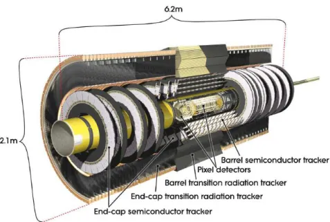
3.4 Inner Detector . . . 36
3.4.1 Pixel Detector . . . 38
3.4.2 SemiConductor Strip Tracker . . . 38
3.4.3 Transition Radiation Tracker . . . 38
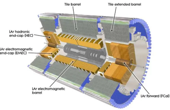
3.5 Calorimeter . . . 39
3.5.2 Electromagnetic Calorimeter . . . 42
3.5.3 Hadronic Calorimeter . . . 43
3.6 Muon Spectrometer . . . 46
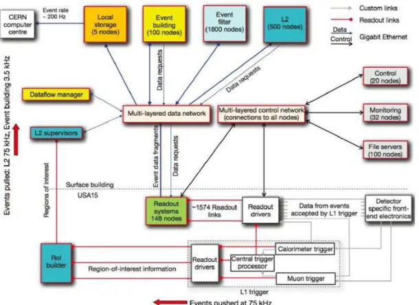
3.7 Trigger and Data Acquisition System . . . 50
3.7.1 Outline of Data Flow . . . 50
3.7.2 Level 1 Trigger System . . . 51
3.7.3 High Level Trigger System . . . 54
3.8 Detector Control System . . . 55
3.9 Pile-up Event . . . 55
3.10 Minimum Bias Event and Underlying Event . . . 56
4 Particle Identification and Event Selection 57 4.1 Electrons . . . 57
4.1.1 Electron Trigger . . . 58
4.1.2 Electron Reconstruction . . . 58
4.1.3 Calorimeter Operating Condition . . . 60
4.1.4 Electron Identification . . . 60
4.1.5 Electron Isolation . . . 62
4.1.6 Detector Alignment . . . 62
4.1.7 Electron Energy Scale . . . 62
4.1.8 Electron Energy Resolution . . . 64
4.1.9 Electron Efficiency Measurement in the Central Region . . . 64
4.2 Muons . . . 68
4.2.1 Muon Trigger . . . 69
4.2.2 Muon Reconstruction . . . 70
4.2.3 Muon Quality Requirement . . . 73
4.2.4 Muon Momentum Scale and Resolution . . . 74
4.3 Jets . . . 78
4.3.1 Cell Clustering Algorithm . . . 78
4.3.2 Jet Reconstruction Algorithm . . . 82
4.3.3 Jet Constituents . . . 84
4.3.4 Local Cluster Weighting Calibration . . . 85
4.3.5 Jet Energy Correction . . . 86
4.3.6 Jet Energy Resolution . . . 98
4.3.7 Track Jet . . . 99
4.3.8 Jet Vertex Fraction . . . 100
4.3.9 b-Flavor Tagging . . . 101
4.3.10 b-Jet Energy Correction . . . 105
4.4 Missing Transverse Energy . . . 110
4.5 Overlap Removal . . . 111
4.6 Event Selection . . . 112
5 Background Estimation 113 5.1 Summary of a Monte Carlo Simulation . . . 113
5.1.1 Event Generator . . . 113
5.1.2 Parton Shower Generator with Event Generator . . . 114
5.1.3 Merging Procedure of Matrix-element and Parton Showering . . . 115
5.1.5 Detector Simulation . . . 119
5.1.6 Configuration . . . 119
5.2 Background Samples . . . 120
5.2.1 Simple Summary . . . 120
5.2.2 Top Quark Pair with Additional Jets . . . 121
5.2.3 Top Quark Pair with Vector Bosons . . . 121
5.2.4 Single Top Quark . . . 121
5.2.5 Vector Bosons with Additional Jets . . . 122
5.2.6 Dibosons . . . 122
5.2.7 Top Quark Pair with Higgs Boson . . . 122
5.2.8 Fake Lepton . . . 123
5.3 Signal Sample of Charged Higgs Bosons . . . 128
5.4 Control and Signal Regions . . . 128
5.5 Boosted Decision Trees Analysis . . . 137
6 Systematic Uncertainties 143 6.1 List of Systematic Uncertainties . . . 143
6.1.1 Systematic Uncertainties for Luminosity Uncertainty . . . 143
6.1.2 Systematic Uncertainties for Reconstructed Objects . . . 145
6.1.3 Systematic Uncertainties on Flavour Tagging . . . 145
6.1.4 Systematic Uncertainties on the Background Estimation . . . 145
6.1.5 Systematic Uncertainties for Monte Calro Modeling of the Signal Process 147 6.2 Fitting Procedure . . . 148
6.2.1 Statistical Test to Search for a New Signal Process . . . 148
6.2.2 Approximate Distribution of the Profile Likelihood Ratio . . . 150
6.2.3 Asimov Data Set . . . 151
6.2.4 CLsMethod with the Statistical Test by Using the Ratio ofLs+bandLb . 152 6.2.5 Likelihood Function in the Control and Signal Regions . . . 154
6.3 Systematic Uncertainties on Fitting Procedure . . . 154
6.4 Post-fit Table and Plots . . . 157
7 Results and Discussions 161 7.1 Estimation of the Sensitivity . . . 161
7.2 Upper Limit Setting . . . 164
7.3 Limit Setting by Using theCLsTechnique . . . 164
7.4 Cross Section Limit . . . 165
7.5 Comparison with the Results from the Other Experiments . . . 166
8 Conclusions 169 A Supplementation in Theory Parts 171 A.1 Crystal-Ball Function . . . 171
A.2 MSSM Benchmark Scenarios after the Discovery of the Higgs Boson . . . 171
A.3 Sudakov Form Factor . . . 173
A.4 Treatment ofW Boson with Two Jets Process . . . 174
A.4.1 Color Flow . . . 174
A.4.2 Leading Logarithmic Term . . . 176
A.5 Parton Distribution Function . . . 177
A.5.2 Parton Parametrization . . . 177
A.5.3 Theoretical Uncertainty . . . 178
A.6 Distributions of Kinematic Variables for the Reweighting intt + jets Samples . . 178
A.6.1 ToppT andtt pT SequentialpT Reweighting . . . 178
A.6.2 tt+b-jets Reweighting by Using the NLO SHERPA Sample . . . 180
B Supplementation in Detector Parts 183 B.1 Absolute Luminosity for ATLAS Detector . . . 183
B.2 Luminosity Algorithms . . . 183
B.2.1 EventOR and EventAND Algorithm . . . 183
B.2.2 Online Algorithm . . . 184
B.3 ATLAS Electronics . . . 184
B.3.1 Front-end Electronics . . . 184
B.3.2 Back-end Electronics . . . 185
List of Figures
1.1 Feynman diagram of the charged Higgs production process for the 4FS. . . 13
1.2 Feynman diagram of the charged Higgs production process for the 5FS. . . 13
1.3 Charged Higgs Branching ratio fortan β = 10 (left) and tan β = 50 (right). . . . 15
1.4 Production cross section multiplied by the branching ratio of H± → tb in the
combination of the 4FS and the 5FS. . . 15
1.5 Summary of the measurements of αs as a function of the energy scale Q. The
brackets indicate the degree of the QCD perturbation theory used in the extraction
ofαs(NLO: the next-to-leading order; NNLO: the next-to-next-to-leading order;
res. NNLO: the NNLO matched with resummed the next-to-leading logs; N3LO:
the next-to-NNLO). The black lines indicateαsevolving fromαs(MZ) =0.1181±0.0011. 18
1.6 Relation between the parton (x, Q2) variables and the kinematic variables
corre-sponding to the final state of the massM produced with the rapidity y at the LHC
collider with √s =14 TeV. The region surrounded by green lines in the figure
indicates the reachable region by utilizing the Hadron-Electron Ring Accelerator
(HERA) and a experiment by using a fixed target. . . 20
1.7 Excluded region oftan β and mH±parameter space in the MSSM for themhmax
scenario. The limit is derived from theH+ → cs and H+ → τν analyses at the
D0 experiment. . . 22
1.8 Excluded region of tanβ and mH±parameter space in the MSSMmmod−
h scenario
for the low mass region (left) and for the high mass region (right). The limit is
derived from theH+→ τ+ν analysis at the ATLAS experiment. . . 23
1.9 Excluded region of tanβ and mH±parameter space in the MSSMmmod−
h scenario
for the low mass region (left) and for the high mass region (right). The limit is
derived from theH+→ tb and H+ → τν analyses at the CMS experiment. . . . 24
2.1 Schematic view of the LHC accelerator chain. . . 29
2.2 Cumulative luminosity versus time forpp collisions at the center of mass collision
energy of 8 TeV during 2012. . . 32
3.1 Schematic view of the ATLAS detector. . . 33
3.2 Interactions between particles and the sub-detectors. . . 34
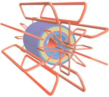
3.3 Schematic view of the magnetic system and the hadronic tile calorimeter system.
The orange color rings indicate the toroid magnets, and the orange color tube located at the most inner cylinder indicates the solenoid magnet. The other tubes indicate the tile calorimeter layers and the outer return yoke. . . 36
3.4 End-cap cryostat system including the calorimeters, feed-throughs and front-end
crates. An outer radius of the cryostat vessel is 2.25 m and a length of the cryostat is 3.17 m. . . 37
3.6 Schematic view of the electromagnetic and the hadronic calorimeters. . . 39
3.7 Schematic view of development of a shower. . . 40
3.8 Electromagnetic calorimeter geometry. . . 42
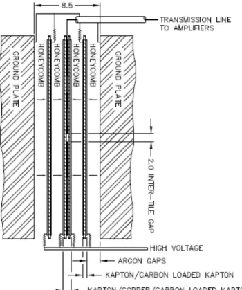
3.9 Schematic view of the hadronic tile calorimeter module. . . 44
3.10 Schematic view of the HEC module. . . 45
3.11 Sectional view of the HEC readout structure. . . 45
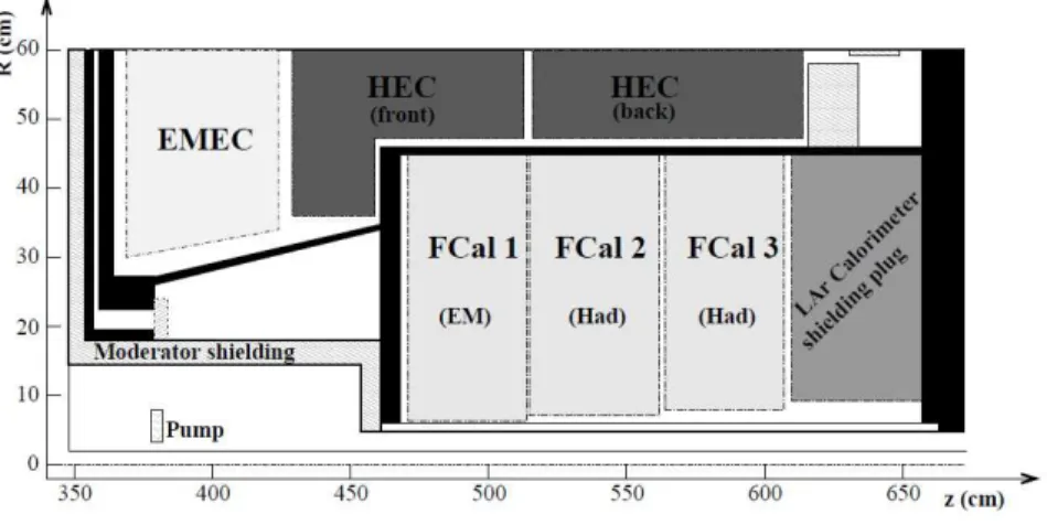
3.12 Sectional view of the Forward Calorimeter and the peripheral detectors. . . 46
3.13 Schematic view of the Muon spectrometer. . . 47
3.14 Schematic view of the muon trigger system. . . 49
3.15 Schematic view of the trigger system and the DAQ system. . . 50
3.16 Level 1 trigger blockdiagram. The red line in the figure indicates a path of the timing, trigger and control distribution (TTC) to detector front-ends. The blue line in the figure indicates a path of the RoI to the L2 trigger. The black dash line in the figure indicates a path to the DAQ. . . 51
3.17 Signal and the readout chain of the L1 barrel muon trigger. . . 53
3.18 4 × 4 sliding window algorithm on the cluster processor of the calorimeter trigger. 54 3.19 Schematic view of theETlocal maximum test for a cluster. . . 54
3.20 Schematic view of the Jet trigger algorithm. The shaded area indicates the RoI for a jet. . . 55
4.1 Trigger efficiency of the electron at the Level 1 trigger with the trigger options, which are L1 EM16 and L1 EM16VH, in the region of|η| < 2.47. We measure the efficiency by using the data at pp collisions of 7 TeV and with an integrated luminosity of 2.4 fb−1. . . 59
4.2 Electron identification efficiency, which is obtained by multiplying the combined scale factor by the efficiency computed from the Z → e−e+ MC simulation, is expressed by a function ofη (coarse binning) on the transverse momentum region 40 < ET < 45 GeV. The black plots indicate loose selection, the red plots indicate medium selection, the blue plots indicate tight selection. . . 69
4.3 Efficiency of the single muon triggers, which are mu24i and mu36, in the region of|η| < 1.05. We measure the efficiency by using the data at pp collisions of 8 TeV and with an integrated luminosity of 20.3 fb−1. The error band of the MC simulation includes both statistic and systematic errors. The lower panel shows the ratio of the data and MC simulation efficiencies. . . 71
4.4 Efficiency of the single muon triggers, which are mu24i and mu36, in the region of|η| > 1.05. We measure the efficiency by using the data at pp collisions of 8 TeV and with an integrated luminosity of 20.3 fb−1. The error band of the MC simulation includes both statistic and systematic errors. The lower panel shows the ratio of the data and MC simulation efficiencies. . . 71
4.5 Muon reconstruction efficiency as a function of η. The muons originate from Z → µ−µ+events and havep T > 10 GeV. The different color plots indicate the type of muon reconstruction. We employ the Chain1 for the reconstruction. The plots for the CaloTag muons are only shown in the region of|η| < 1. The error bars in the upper panel indicate the statistical uncertainty. The plots in the lower pannel show the ratio between the efficiency derived from the MC simulation and the data. The error bars in the lower panel indicate the combination of the statistical and systematic uncertainties. . . 73
4.6 Noise distributions for the 2010 operations are evaluated by using the MC
simula-tion with the average ofpp collisions per bunch crossing of µ = 0 and the center
of mass collision energy of 7 TeV. The distribution is shown as a function of|η|. The different colours indicate the different type of the calorimeters and layers. . . 80
4.7 Noise distributions for the 2011 operations are evaluated by using the MC
simula-tion with the average ofpp collisions per bunch crossing of µ = 8 and the center
of mass collision energy of 7 TeV. The distribution is shown as a function of|η|. The different colours indicate the different type of the calorimeters and layers. . . 80
4.8 Schema of a precluster pair in the anti-kt algorithm. . . 84
4.9 Average reconstructed transverse momentumpjetT,EM on the EM scale for jets in
MC simulations as a function of the number of reconstructed primary vertices
NPVand7.5 ≤ µ < 8.5 in various bins of a truth-jet transverse momentum ptruthT . 89 4.10 Average reconstructed jet transverse momentumpjetT, EMon the EM scale as a
func-tion of the average number of collisionsµ at a fixed number of primary vertices
NPV = 6. . . 89 4.11 Average jet energy response for the EM-scale as a function of|ηdet|. The different
color plots correspond to the different jet energy: the green plots are 30 GeV, the black plots are 60 GeV, the yellow plots are 110 GeV, the blue plots are 400 GeV
and the red plots are 2000 GeV. We employ the anti-ktalgorithm withR = 0.6
for the jet clustering. . . 90 4.12 Average difference∆η = ηtruth− ηorigin in(Etruth, ηdet) bins as a function of
|ηdet| and EEM+JESjet . . . 91 4.13 Relative jet response1/c to the probe jet with 40 ≤ pavgT ≤ 55 GeV as a function
of the probe jetηdetby using the central reference method and the matrix method. We employ the probe jets calibrated by the EM+JES scale and reconstructed by
the anti-ktalgorithm withR = 0.4. The lower panel shows the ratio of the MC
simulation and the data. . . 94 4.14 R(pjetT , η) derived from the mean pT balance in Z+jets events as a function of
the reference jetpT by using the MC simulation generated by PYTHIA and the
data taken at the center of mass collision energy of 7 TeV and with an integrated luminosity of 4.7 fb−1. The gray band indicates the total uncertainty. . . 95 4.15 Average jet responsehpjetT /pγTi, which is measured by the DB method, to γ+jets
events as a function of the photon transverse momentum. The lower panel shows the ratio of the MC simulation and the data. The error bars on the plots indicate the statistical uncertainty. . . 96
4.16 Average jet responsehRMPFi, which is measured by the MPF method, to γ+jets
events as a function of the photon transverse momentum. The lower panel shows the ratio of the MC simulation and the data. The error bars on the plots indicate the statistical uncertainty. . . 96 4.17 Systematic uncertainties on the ratio of the MC simulation and the data measured
by the DB method. . . 97
4.18 Systematic uncertainties on the ratio of the MC simulation and the data measured
4.19 Multiple jets balance as a function of the recoil systemprecoilT by using the MC simulation generated by the PYTHIA and the data taken at the center of mass col-lision energy of 7 TeV and with an integrated luminosity of 4.7 fb−1. The circular plots in the lower panel show the ratio of the MJB between the MC simulation and the data. The green line in the lower panel shows the ratio of the calorimeter response, which is the ratio of the jetpTand the reference photonpγTor the refer-enceZ boson pZT, between the MC simulation and the data as a function of thepγT
orpZT. . . 98
4.20 Definition of coordinates and variables used in the bi-sector technique. . . 99
4.21 Left and right plots show the light-flavor jet rejection and the c-jet rejection as a function of the b-tag efficiency, respectively. We derive the efficiencies from the MC simulation sample of thett single lepton and dilepton events with pT > 15 GeV and |η| < 2.5 at pp collisions of 7 TeV. . . 101
4.22 Distribution of the dilepton invariant mass in theeµ + 2 jets channel. . . 103
4.23 Distribution of the transverse momentum of the dilepton system in theeµ + 2 jets channel. . . 103
4.24 Distribution of the jetpTin theeµ + 2 jets channel. . . 103
4.25 Distribution of the jetη in the eµ + 2 jets channel. . . 103
4.26 b-tag efficiency of the data and simulation. . . 106
4.27 b-tag scale factor as a function of the b-jet pT. . . 106
4.28 Calorimeter responseRrtrk tob-jets in the inclusive jets sample as a function of the jetpT. . . 108
4.29 Calorimeter responseRrtrk tob-jets in the tt sample as a function of the jet pT. . 108
4.30 Difference in the calorimeter response betweenb-jets and inclusive jets by using the inclusive jets sample. . . 108
4.31 Difference in the calorimeter response betweenb-jets and light-flavor jets by using thett sample. . . 108
4.32 Relative response of theb-jets with semileptonic decay B hadron decays to the inclusiveb-jets as a function of the average pTof dijet. . . 109
5.1 Hard scattering event along with the underlying event from remnant particles and gluon emissions in app collision. . . 114
5.2 Schematic view of the merging procedure in the CKKW thechnique. . . 117
5.3 MSTW 2008 NLO Parton Distribution Functions at scales ofQ2 = 10 GeV2and Q2 = 104GeV2with the one-sigma-confidence-level-uncertainty bands related to theαsuncertainty. . . 119
5.4 Single top production process at the NLO level is described as the subsequent top decay in the thett pair production. . . 122
5.5 Real efficiencyεrand fake efficiencyεf in thee+jets channel as functions of the different variables and the trigger options. The variables are electron cluster eta |η|e, electron transverse energypeT, and the minimum∆R between electron and jets. e60 indicates high pT trigger, e24vh indicates lowpT trigger without the isolation cut, e24vhi indicates lowpTtrigger with the isolation cut. . . 126
5.6 Real efficiency εr and fake efficiency εf in the e+jets channel as functions of the different variables and the trigger options. The variables are leading jet pT
pleading jetT , the number of jets njet, the number of b-tagged jets nb-jet, and the
angle in the transverse plane between the electron and the MET ∆φ(e, ETmiss).
e60 indicates highpTtrigger, e24vh indicates lowpTtrigger without the isolation
cut, e24vhi indicates lowpTtrigger with the isolation cut. . . 126
5.7 Real efficiencyεr and fake efficiencyεf in theµ+jets channel as functions of the different variables and the trigger options. The variables are muon eta|η|µ, muon transverse momentumpµT, and the minimum∆R between muon and jets. mu36 indicates highpTtrigger, mu24 indicates lowpTtrigger without the isolation cut, mu24i indicates lowpTtrigger with the isolation cut. . . 127
5.8 Real efficiency εr and fake efficiency εf in the µ+jets channel as functions of the different variables and the trigger options. The variables are leading jet pT pleading jetT , the number of jetsnjet, the number ofb-tagged jets nb-jet, and the angle in the transverse plane between the muon and the MET ∆φ(µ, ETmiss). mu36 indicates highpTtrigger, mu24 indicates lowpTtrigger without the isolation cut, mu24i indicates lowpTtrigger with the isolation cut. . . 127
5.9 Pie charts for all background compositions in the control and the signal regions. . 130
5.10 HadronicHTon 4 jets and 2b-tags region. . . 131
5.11 HadronicHTon 4 jets and≥ 3 b-tags region. . . 131
5.12 HadronicHTon 5 jets and 2b-tags region. . . 132
5.13 HadronicHTon≥ 6 jets and 2 b-tags region. . . 132
5.14 Average∆Rbbon 4 jets and 2b-tags region. . . 132
5.15 mbbfor theb-pair that is closest in ∆R on 4 jets and 2 b-tags region. . . 132
5.16 Second Fox-Wolfram moment calculated from the jets on 4 jets and 2b-tags region. 133 5.17 pTof the leading jet on 4 jets and 2b-tags region. . . 133
5.18 Average∆Rbbon 4 jets and≥ 3 b-tags region. . . 133
5.19 mbbfor theb-pair that is closest in ∆R on 4 jets and ≥ 3 b-tags region. . . 133
5.20 Second Fox-Wolfram moment calculated from the jets on 4 jets and≥ 3 b-tags region. . . 134
5.21 pTof the leading jet on 4 jets and≥ 3 b-tags region. . . 134
5.22 Average∆Rbbon 5 jets and 2b-tags region. . . 134
5.23 mbbfor theb-pair that is closest in ∆R on 5 jets and 2 b-tags region. . . 134
5.24 Second Fox-Wolfram moment calculated from the jet on 5 jets and 2b-tags region. 135 5.25 pTof the leading jet on 5 jets and 2b-tags region. . . 135
5.26 Average∆Rbbon≥ 6jets and 2 b-tags region. . . 135
5.27 mbbfor theb-pair that is closest in ∆R on ≥ 6 jets and 2 b-tags region. . . 135
5.28 Second Fox-Wolfram moment calculated from the jets on≥ 6 jets and 2 b-tags region. . . 136
5.29 pTof the leading jet on≥ 6 jets and 2 b-tags region. . . 136
5.30 Schematic view of a decision tree.xi, xj, and xk represent discriminant variables. c1, c2, and c3 indicate the best points to discriminate between a signal process and a background process. The algorithm starts from the root node. An event is classified into the one of the leaf nodes at the bottom end of the tree for signal, labelled as S in the figure, or the leaf nodes at the bottom end of the tree for background, labelled as B in the figure. . . 137
5.31 Distributions of background-like events and signal-like events, which originate from charged Higgs bosons with mass of 500 GeV, in the BDT input variables. . 140
5.32 Second Fox-Wolfram moment calculated from the jets. . . 141
5.33 Average∆Rbb. . . 141
5.34 pTof the leading jet. . . 141
5.35 mbbfor theb-pair that is closest in ∆R. . . 141
5.36 HadronicHT. . . 141
5.37 Distribution of the BDT output on 300 GeV. . . 142
5.38 Distribution of the BDT output on 500 GeV. . . 142
6.1 Illustration of the relation between the observedtµvalue and thep value. . . 150
6.2 Illustration of the relation between the Z and thep value. . . 150
6.3 Post-fit pulls and the impact on the measured signal strength of the 15 most rele-vant uncertainties on the signal plus background hypothesis ofmH±= 300 GeV. 155 6.4 Post-fit pulls and the impact on the measured signal strength of the 15 most rele-vant uncertainties on the signal plus background hypothesis ofmH±= 500 GeV. 155 6.5 Correlation plot between the nuisance parameters and the signal strength on the three mass hypotheses ofmH± = 200, 400, and 600 GeV. . . 156
6.6 Hadronic Ht on 4 jets and 2b-tags region. . . 158
6.7 Hadronic Ht on 4 jets and 3b-tags region. . . 158
6.8 Hadronic Ht on 5 jets and 2b-tags region. . . 158
6.9 Hadronic Ht on 6 jets and 2b-tags region. . . 158
6.10 Distribution of the BDT output on 300 GeV. . . 158
6.11 Distribution of the BDT output on 500 GeV. . . 158
6.12 Distribution of the BDT output withmH+ of 300 GeV on 4 jets and 2b-tags region.159 6.13 Distribution of the BDT output withmH+ of 300 GeV on 4 jets and 3b-tags region.159 6.14 Distribution of the BDT output withmH+ of 300 GeV on 5 jets and 2b-tags region.159 6.15 Distribution of the BDT output withmH+ of 300 GeV on 6 jets and 2b-tags region.159 6.16 Hadronic Ht distribution on the signal region. . . 160
7.1 Illustration of thep-value corresponding to the median of qµassuming a strength parameterµ′. . . 161
7.2 Upper limits on the production cross section,σ(gb → tH+) × BR(H+→ tb), for charged Higgs bosons. . . 165
7.3 Observed localp0value in the search forgb → tH+withH+→ tb. . . 166
7.4 Upper limits on the production cross section,σ(gb → tH+) × BR(H+ → τ+ν), from ATLAS charged Higgs analysis at√s = 8 TeV. . . 167
7.5 Upper limits on the production cross section, σ(gb → tH+) × BR(H+ → tb), including the expected limit without systematic uncertainty. . . 167
7.6 Upper limits on the production cross section,σ(pp → t(b)H+) × Br(H+→ tb), in semileptonic channel for charged Higgs bosons at √s = 8 TeV at the CMS experiment. . . 168
7.7 Upper limits on the production cross section,σ(pp → tH+) × BR(H+ → tb), in combined channels for charged Higgs bosons at√s = 8 TeV at the CMS experiment.168 A.1 Feynman diagrams for theW boson + two jets process. The upper processes has a gluon emission from the internal line. The lower processes has a gluon emission from the external line. . . 175
A.2 Two examples of the color flow in theW boson + two jets process with the soft gluon p1. The left diagram is the leading color flow. The right diagram is the sub-leading color flow. . . 176
A.3 Normalized differential cross section for the transverse momentum of the hadroni-cally decaying top quark. The green circles indicate the values from ALPGEN+HERWIG. The red squares indicate the values from MC@NLO+HERWIG. The blue circles indicate the values from POWHEG+HERWIG. The pink triangles indicate the values from POWHEG+PYTHIA. The gray bands indicate the total uncertainty on the data in each bin. . . 179
A.4 Normalized differential cross section for the transverse momentum of thett
sys-tem. The green circles indicate the values from ALPGEN+HERWIG. The red squares indicate the values from MC@NLO+HERWIG. The blue circles indicate the values from POWHEG+HERWIG. The pink triangles indicate the values from POWHEG+PYTHIA. The gray bands indicate the total uncertainty on the data in each bin. . . 179 A.5 Differential cross section for the transverse momentum of the first light-flavour jet. 180 A.6 Differential cross section for the invariant mass of the first and secondb-flavour jets.180
A.7 Differential cross section for the transverse momentum of the first b-flavour jet. . 181
List of Tables
1.1 Properties of quarks and leptons. . . 2
1.2 Properties of gauge bosons. . . 2
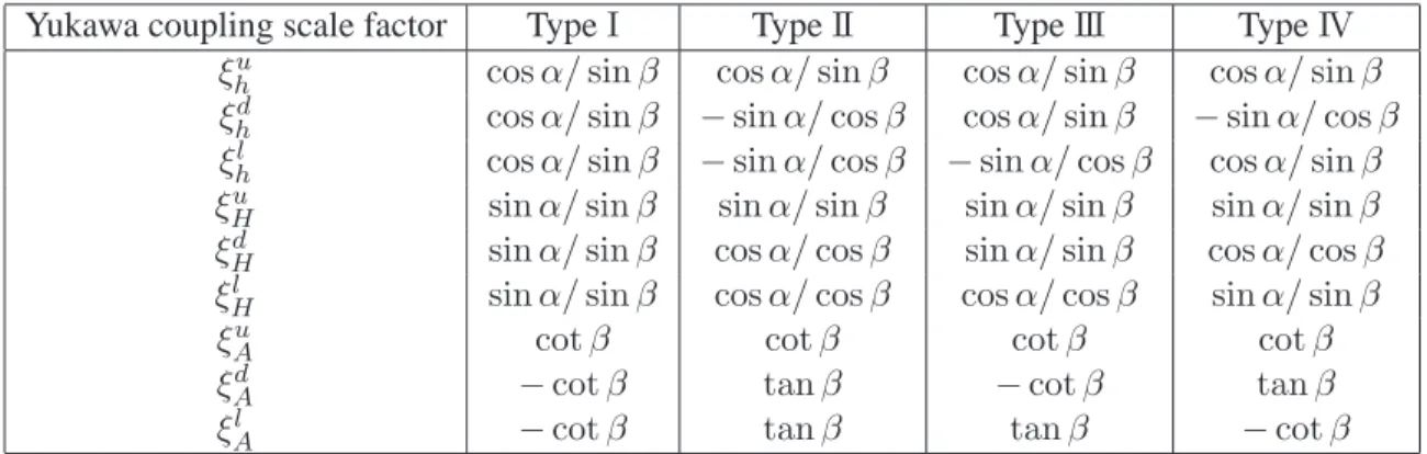
1.3 Yukawa couplings to the fermions in four types of the THDM. . . 12
2.1 Summary of the LHC main parameters. . . 28
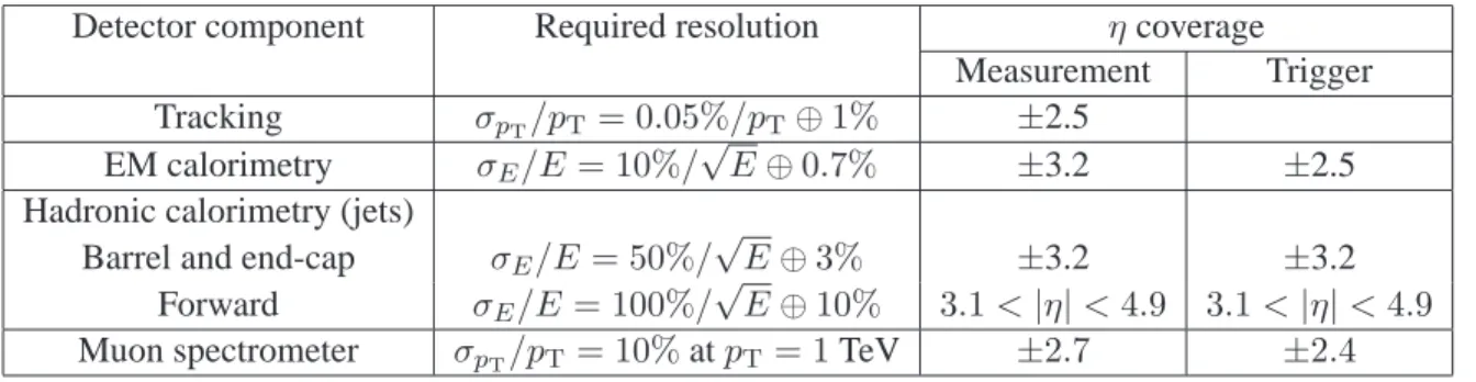
3.1 Requirement for the detector components in the ATLAS detector. . . 35
3.2 Main parameters of the pixel detector. . . 38
3.3 Main parameters of the SCT. . . 39
3.4 Granularity and coverage of the electromagnetic calorimeters. . . 43
3.5 Main parameters of the hadronic tile calorimeter. . . 43
3.6 Main parameters of the FCal modules. . . 46
4.1 Definition of variables used for the identification selection. . . 61
4.2 Parameters of a tower building for the electromagnetic calorimeter (EM) and a
combination of electromagnetic and hadronic calorimeters (Combined) in the
win-dow algorithm. . . 78
4.3 Parameters of the precluster finding for the EM calorimeter in the window algorithm. 79
4.4 Cluster sizeNηcluster×Nφclusterfor different particle types in the barrel and end-cap regions. . . 79 4.5 Parameters used to build two types of the topological cluster available in the
stan-dard ATLAS reconstruction. . . 81
5.1 Pre-fit number of events for the background and the signal processes in all regions. The upper rows indicate the numbers in the muon channel. The lower rows indi-cate the numbers in the electron channel. The uncertainty in the table includes the only statistic uncertainty.±0 in the “Tot. data” row indicates that the obtained-real
data is just a number. . . 129
5.2 Options for the BDT training. . . 138
6.1 Summary of systematic uncertainties. . . 144
6.2 Fractional uncertainties on the signal strength for various systematic sources. . . 155
6.3 Post-fit number of events for the background and the signal processes in all
re-gions. We sum the numbers in the muon channel and the numbers in the electron channel. The uncertainty in the table includes the statistic and systematic uncer-tainties. ±0 in the “Tot. data” row indicates that the obtained-real data is just a number. . . 157
7.1 Comparison of expected 95 % CL limits on σ(gb → tH+) × BR(H+ → tb)
Chapter 1
Introduction
Symmetry and relativeness are essential principles in modern particle physics. Concept of symmetry breaking brought reasonable explanations to unexplained phenomena. Now, we try to explain some unsolved issues such as hierarchy problem and dark matter by introducing a new symmetry, Supersymmetry (SUSY), and its breaking. However, we have not discovered a new particle from the symmetry yet. It is important for us to search for a SUSY particle, but I think how to break symmetry is also important. Prof. Nambu imported the concept of the symmetry breaking in particle physics from the superconductivity in solid state physics. Prof. Nambu’s intuition that particle physics has relation with solid state physics is great. Superconductivity has complex phenomena such as ferromagnetic superconductors and odd frequency superconductors. In addition to this complexness of the system with symmetry breaking, there is a room to expand the Standard Model Higgs sector with only one Higgs doublet. It is a motivation of this charged Higgs bosons search to consider new extended Higgs sectors.
1.1
Gauge Bosons and Fermions
There are variety of things in the world. In spite of this diversity, all things are composed of leptons and quarks, and all interactions are mediated by gauge bosons in the sight of particle physics that deals with the very small particle, smaller than atomic scale. Four force fields, elec-tromagnetic, weak, strong, and gravitational fields, control interactions between particles. The Standard Model treats three interactions, electromagnetic and weak and strong interactions. Mod-ern particle physics is based on gauge symmetry related with the force fields [1, 2]. There are fermions which are half integer spin particles obeying Fermi-Dirac statistics and bosons which are integer spin particles obeying Bose-Einstein statistics. The bosons can be categorized by their spin and parity eigenvalues: scalar bosons with spin zero like Higgs boson, and vector bosons with spin one like gluon. The fermions are composed of quarks and leptons with the different interaction to the gauge bosons.
Massless photon mediates electromagnetic interaction. MassiveW± andZ bosons mediate
weak interaction. Massless gluon mediates strong interaction. Leptons do not couple with gluon, but quarks couple with gluon. Strong interaction is based on non-Abelian gauge field and this causes the quark confinement, therefore we cannot extract only one quark from nucleon. Quarks and leptons are described as isospin doublets in the Standard Model and there are three genera-tions. The particles of different generations have different masses, and the third generation is the heaviest. Quarks tend to have heavier masses than leptons in the same generation. Quarks are classified to six flavours, up and down, charm and strange, top and bottom. Leptons are classified
to six particles, electron and electron neutrino, muon and muon neutrino, tau and tau neutrino. Table 1.1 shows properties of quarks and leptons. Through weak interaction, quarks and leptons can change their flavours. However, flavor changing neutral current is strongly suppressed.
Table 1.1: Properties of quarks and leptons.
Generation Properties
1st 2nd 3rd Spin Electric charge Interaction
Quark u c t 1/2 +2/3 EM, Weak, Strong
d s b 1/2 −1/3 EM, Weak, Strong
Lepton νe νµ ντ 1/2 0 Weak
e µ τ 1/2 −1 EM, Weak
The gauge interactions have charges which are required from symmetry of the fields. The charges must conserve before and after the interactions. If a particle does not have a charge, the gauge boson related with the charge cannot interact with the non-charge particle. The distance of interactions is different between interactions. Photon can propagate to infinity. Gluon can
propa-gate to color confinement range. W±,Z bosons can propagate to the distance related with their
inverse masses. Table 1.2 shows properties of gauge bosons. The mass of gluon is a theoretical value.
Table 1.2: Properties of gauge bosons.
Gauge boson Force Spin Electric charge Mass
g (gluon) Strong 1 0 0 [3]
γ (photon) EM 1 0 < 1 × 10⁻¹⁸eV [3]
W±(weak bosons) Weak 1 ±1 80.385±0.015 GeV [3]
Z (weak boson) Weak 1 0 91.1876±0.0021 GeV [3]
Gauge theory requires that gauge boson is massless. This is a contradiction to the fact that weak gauge bosons have masses. If it were not for the Higgs mechanism, we would find a problem that the scattering amplitude between longitudinal W± bosons in s-channel, WL+WL− → WL+WL−,
becomes proportional tos, the center of mass collision energy for the process, and would diverge
at larges. We would also find another problem related to the origin of the fermion mass, where the
mass term of Lagrangian breaks invariance for a chiral transformation. To solve those problems related to gauge boson and fermion, the Higgs mechanism was introduced.
1.2
Standard Model and Higgs Boson
The Higgs boson plays an important part in the mechanism of giving mass to particles on
SU (2)L× U(1)Y gauge interactions. A simple summary of the Weinberg-Salam theory with the Higgs mechanism is described as follows. Potential of a complex scalar field has spontaneously breaking of symmetry, which is proposed by Nambu [4, 5]. All gauge bosons and fermions are massless before the symmetry breaking. The potential of the scalar field changes at a transition temperature for the symmetry breaking, and a vacuum state satisfying the symmetry drops into a
new vacuum state, which does not satisfy the symmetry. The broken potential looks like bottom of a wine bottle, and the breaking process seems that a state on the top of the convex fall to a state on the bottom of the concavity around the convex. In this breaking process, the Nambu-Goldstone boson, which is component of the complex scalar field at the bottom state, is eaten by
masslessSU (2)LandU (1)Y gauge bosons corresponding to the weak bosons and the photon. The
SU (2)LandU (1)Y gauge bosons get to have the longitudinal state. Therefore, the gauge bosons become massive. Using the analogy of a wine bottle, a freedom of rotating around the convex represents the Nambu-Goldstone boson and fixing the rotating state to the particular point of the bottom represents eating of the Nambu-Goldstone boson by the massless gauge bosons. This is the key point of the Higgs mechanism. Equations (1.1) and (1.2) express the process of eating
Nambu-Goldstone boson by using simpleU (1) equation,
φ = r 1 2(v + η(x) + iξ(x)) (1.1) ≃ r 1 2(v + η(x)) exp (iξ(x)/v), (1.2)
whereφ is a complex scalar field on U (1), v is an expectation value, and x indicates a parameter
ofU (1) local gauge transformation. η is the real part of fluctuation around v, and this real field is
called the Higgs field in the Standard Model.ξ in Equation (1.1) indicates fluctuation of the scalar
field along complex axis like Nambu-Goldstone boson. ξ is shown to be the phase variation on
U (1) local gauge transformation in Equation (1.2). This formula deformation also indicates that
φ → φ exp (iξ(x)/v), (1.3)
Aµ → Aµ+ 1
e∂µ ξ(x)
v , (1.4)
whereAµisU (1) gauge field with a charge e. By fixing the particular gauge, which remains the
only real part of the complex scalar field, the filed shown in Equation (1.3) becomesp1/2(v +
η(x)), furthermore the U (1) gauge filed loses a degree of freedom related to the gauge
transfor-mation. The fixing leads to the symmetry breaking of the gauge symmetry.
One of theSU (2)Lfields and theU (1)Y field are mixed by the Weinberg-Salam angle. This
mixing leads to mixing the right-handed and left-handed components in weak neutral current,
and the vacuum state is unbroken forU (1)em gauge transformations with a charge operator Q≡
T3+ Y/2. Two of the SU (2)Lfields are mixed by making the weak charged currents. Finally, we
get three massive weak bosons,Z and W±, and one massless boson,γ. The Higgs boson is the
fluctuation to a remained component of the complex scalar field around the vacuum expectation. Masses of fermions are given by Yukawa coupling, the Higgs boson mediates the interaction between left-handed fermions and right-handed fermions. fermion mass terms in the Standard Model Lagrangian is characterized by the Yukawa coupling constant, the Higgs field, and the expectation value. After the vacuum expectation value getting non-zero value, fermion masses become non-zero, in other wards, the left-handed states and the right-handed states are mixing. Therefore, the vacuum phase transition leads to breaking of the chiral symmetry of fermions.
The Standard Lagrangian on the Weinberg-Salam model after the symmetry breaking is ex-pressed by
L = −14Wµν· Wµν− 1 4Bµν · B µν + Lγµ(i∂µ− g1 2τ · Wµ− g ′Y 2Bµ)L + Rγµ(i∂µ− g′ Y 2Bµ)R + |(i∂µ− g1 2τ· Wµ− g ′Y 2Bµ)φ| 2 − V (φ) − (G1LφR + G2LφcR+ hermitian conjugate), (1.5) with Wµν = ∂µWν− ∂νWµ− gWµ× Wν, (1.6) Bµν = ∂µBν− ∂νBµ, (1.7) g′/g = tan θW, (1.8) V (φ) = µ2φ†φ + λ(φ†φ)2+ · · · , with µ2 < 0 and λ > 0, (1.9) φ = Ã 0 v+h(x) √ 2 ! , φc= Ã v+h(x) √ 2 0 ! . (1.10)
The first and second terms in Equation (1.5) indicate theW±,Z, and γ kinematic energies and
self-interactions. Wµis anSU (2)Lvector composed of three gauge fields,Wµawitha = 1, 2, 3.
Bµis aU (1)Y vector boson. Under a local gauge transformation ofSU (2)L, which is expressed by α(x) (αa(x) with a = 1, 2, 3), Wµtransforms as
Wµ → Wµ− 1
g∂µα(x) − α(x) × Wµ. (1.11)
Under a local gauge transformation ofU (1)Y, which is expressed byβ(x), Bµtransforms as
Bµ → Bµ−
1
g′∂µβ(x). (1.12)
α× Wµterm in Equation (1.11) means that Wµrotates around an orthogonal axis to a α-Wµ
plane by the non-Abelian gauge transformation α. The third and fourth terms in Equation (1.5)
indicate lepton and quark kinematic energies and their interactions withW±, Z, γ. R is
right-handed quark singlets and right-right-handed lepton singlets, and L is left-right-handed quark doublets and left-handed lepton doublets. τ indicates the Pauli spin matrices. Y is a generator of theU (1)Y
gauge field. g is a coupling constant between the SU (2)Lgauge field and the weak isospin
cur-rent,g′ is a coupling constant between theU (1)Y gauge field and the hypercharge current. The
Weinberg-Salam angle,θW, is determined by experiment. Under a local gauge transformation of
theSU (2)L× U(1)Y, the left-handed and right-handed components are transformed as
L→ exp(iα(x) · T + iβ(x)Y)L, (1.13)
We can transform the third and fourth terms in Equation (1.5) as Lγµ(i∂µ− g1 2τ· Wµ− g ′Y 2Bµ)L + Rγ µ(i∂ µ− g′Y 2Bµ)R = iψγµ∂µψ − g 1 2Lγ µτ · W µL− g′ψγµ Y 2Bµψ = iψγµ∂µψ − gψγµT· Wµψ − g′ψγµY 2Bµψ = iψγµ∂µψ − gJµweak· Wµ− g′ JµhyperBµ 2 = iψγµ∂µψ − g(J1, weakµ W1, µ+ J2, weakµ W2, µ)
− Ã g′J µ hyperBµ 2 + gJ µ 3, weakW3, µ ! , (1.15) with ψ = L + R, ψ = L + R. (1.16)
T is a generator of theSU (2)Lgauge field. The second term in Equation (1.15) becomes
J1, weakµ W1, µ+ J2, weakµ W2, µ = Lγµ1 2(τ1W1, µ+ τ2W2, µ)L = Lγµ r 1 2(τ+W + µ + τ−Wµ−)L = r 1 2(J µ +, weakWµ++ J−, weakµ Wµ−), (1.17) where τ+ = 1 2(τ1+ iτ2), τ− = 1 2(τ1− iτ2), (1.18) Wµ+= r 1 2(W1, µ− iW2, µ), W − µ = r 1 2(W1, µ+ iW2, µ), (1.19) J+, weakµ = Lγµτ+L, J−, weakµ = Lγµτ−L. (1.20) J±,weakµ andW±
µ indicate the charged currents and W± bosons in the electroweak interaction,
respectively. The third term in Equation (1.15) becomes
g′Jhyperµ Bµ 2 + gJ µ 3, weakW3, µ = Ã g sin θWJ3, weakµ + g′cos θWJhyperµ 2 ! Aµ + Ã g cos θWJ3, weakµ − g′sin θWJµ hyper 2 ! Zµ, (1.21) where
Aµ = cos θWBµ+ sin θWW3, µ, (1.22)
Zµ = − sin θWBµ+ cos θWW3, µ. (1.23)
θW indicates the Weinberg-Salam angle. By substituting Jemµ = J3, weakµ +
Jhyperµ
2 with Q ≡
T3+ Y/2, the final form of the third term in Equation (1.15) becomes
eJemµ Aµ+ e sin θWcos θW (J3, weakµ − sin2θWJemµ )Zµ, (1.24) where e = g sin θW (1.25) = g′cos θW. (1.26)
AµandZµcorrespond to the photon and theZ boson, Jemµ is the electromagnetic current. We go back to Equation (1.5): −14Wµν · Wµν− 1 4Bµν· B µν = −1 4[(∂µWν − ∂νWµ− gWµ× Wν) · (∂ µWν − ∂νWµ− gWµ× Wν) +Bµν· Bµν]. (1.27)
Then, we consider the component without terms related with the vector product Wµ× Wν:
(∂µWν− ∂νWµ) · (∂µWν − ∂νWµ) + Bµν· Bµν = (∂µWν,1− ∂νWµ,1)(∂µW1ν− ∂νW1µ) + (∂µWν,2− ∂νWµ,2)(∂µW2ν− ∂νW2µ) +(∂µWν,3− ∂νWµ,3)(∂µW3ν − ∂νW3µ) + (∂µBν− ∂νBµ)(∂µBν − ∂νBµ) = 2(∂µWν+− ∂νWµ+)(∂µW−,ν− ∂νW−,µ) +(∂µZν − ∂νZµ)(∂µZν − ∂νZµ) + (∂µAν − ∂νAµ)(∂µAν − ∂νAµ) = 2Wµν+W−,µν+ ZµνZµν+ FµνFµν, (1.28)
where we use some deformations such as
∂µWν,1∂µW1ν + ∂µWν,2∂µW2ν = ∂µWν,1∂µW1ν+ i∂aW1b∂aW2,b− i∂aW1b∂aW2,b+ ∂µWν,2∂µW2ν
= ∂µWν,1∂µW1ν+ igaµgaµ′gbνgbν′∂µW1,ν∂µ ′
W2ν′ −i∂aW2,b∂aW1b+ ∂µWν,2∂µW2ν
= ∂µWν,1(∂µW1ν + i∂µW2ν) − i∂µWν,2(∂µW1ν+ i∂µW2ν)
= (∂µWν,1− i∂µWν,2)(∂µW1ν+ i∂µW2ν)
= 2∂µWν+∂µW−,ν (1.29)
∂µWν,3∂µW3ν+ ∂µBν∂µBν = sin2θW∂µWν,3∂µW3ν + cos2θW∂µBν∂µBν
+ cos2θW∂µWν,3∂µW3ν+ sin2θW∂µBν∂µBν
= sin2θW∂µWν,3∂µW3ν+ cos θWsin θW∂µBν∂µW3,ν
+ sin θWcos θW∂µW3ν∂µBν + cos2θW∂µBν∂µBν
+ cos2θW∂µWν,3∂µW3ν− cos θWsin θW∂µBν∂µW3,ν
− sin θWcos θW∂µW3ν∂µBν+ sin2θW∂µBν∂µBν
= ∂µ(cos θWBν+ sin θWW3ν)∂µ(cos θWBν+ sin θWW3,ν)
+∂µ(− sin θWBν + cos θWW3ν)∂µ(− sin θWBν+ cos θWW3,ν)
= ∂µAν∂µAν+ ∂µZν∂µZν. (1.30)
Equation (1.28) indicates kinetic energies of W±, Z, and γ. The term related with the vector
product, which is removed from the above calculation, indicates the self interactions.
The fifth, sixth and seventh terms in Equation (1.5) indicate W±, Z, γ, and Higgs boson
masses and the Yukawa couplings, respectively. The vacuum expectation value of the Higgs
dou-blet withT = 1/2, T3 = −1/2, and Y = 1 is written as
hφi = r 1 2 µ 0 v ¶ , (1.31)
wherev is the vacuum expectation value, v = 246 GeV. This provides masses of the gauge bosons
by ¯ ¯ ¯ ¯ µ i∂µ− g 1 2τ · Wµ− g ′Y 2Bµ ¶ φ ¯ ¯ ¯ ¯ 2 = 1 2 ¯ ¯ ¯ ¯ µ −g12τ· Wµ− g′ 1 2Bµ ¶ µ 0 v ¶¯¯¯ ¯ 2 = 1 8 ¯ ¯ ¯ ¯ µ gWν,3+ g′Bµ g(Wν,1− iWν,2) g(Wν,1+ iWν,2) −gWν,3+ g′Bµ ¶ µ 0 v ¶¯¯¯ ¯ 2 = 1 8v 2g2[(W µ,1)2+ (Wµ,2)2] + 1 8v 2(g′B µ− gWµ,3)(g′Bµ− gWµ,3) = (1 2vg) 2W+ µWµ,−+ 1 8v 2(gW µ,3− g′Bµ)2+ 0(gWµ,3+ g′Bµ)2. (1.32)
In Equation (1.32),vg/2 in the first term indicates W±mass,vpg2+ (g′)2/2 in the second term
indicates Z mass, and 0 in the third term indicates photon mass. V (φ) in Equation (1.5) is the
scalar potential with the Higgs field after the symmetry breaking, andφ is the Higgs doublet after
the symmetry breaking.µ2is the parameter related with the Higgs boson mass, which is expressed
byp−2µ2. µ2 has a positive value before the symmetry breaking and has a negative value after
the symmetry breaking. λ is a coupling strength for the self coupling. The charge conjugation
Higgs doublet is expressed by−iτ2φ∗. Therefore, the charge conjugation doublet hasY = −1.
h(x) is the Higgs field. The Higgs boson mass is also expressed by m2h = 2v2λ.
For fermion mass terms related with the up quark and the down quark, the interaction between the Higgs potentialφ and the quarks is expressed by
[G1LφR + G2LφcR+ hermitian conjugate]up-quark, down-quark = r 1 2Gd ¡ u, d ¢L µ 0 v + h(x) ¶ dR+ r 1 2Gu ¡ u, d ¢L µ v + h(x) 0 ¶ uR + r 1 2GddR ¡ 0, v + h(x) ¢ µ u, d ¶ L + r 1 2GuuR ¡ v + h(x), 0 ¢ µ u, d ¶ L = r 1 2Gd(dLdR+ dRdL)(v + h(x)) + r 1 2Gu(uLuR+ uRuL)(v + h(x)), (1.33)
whereGdandGu are coupling constants between down quark and the Higgs field, up quark and
the Higgs field, respectively. In this calculation, L, R, L and R indicate not the flavour eigen state but the mass eigen state. The coupling constants are also expressed by
Gd= md √ 2 v , Gu= mu √ 2 v , (1.34)
wheremdandmuare masses of the down quark and up quark, respectively.
The existence of the Higgs boson was the last piece for the Standard Model. In 2012 year, the ATLAS and the CMS collaborations published the discovery of the Higgs boson [6–8].
1.3
Beyond the Standard Model
We discovered the Higgs boson, and the Standard Model became more robust. However, there are some unsolved issues such as hierarchy problem and dark matter in the Standard Model. Therefore, we need the Beyond Standard Model (BSM). We can expand the Higgs sector in the Standard Model because there is no reasons for the minimal Higgs sector. In order to achieve the expansion of the Higgs sector, we must satisfy requirements from two experimental observation facts:
• ρ parameter, which represents the relative strength of the weak neutral interaction to the
weak charged interaction, is one.
• There is no Flavour Changing Neutral Current (FCNC) at the tree level.
The ρ parameter is expressed by using the Weinberg-Salam angle θW, a Higgs isospinIi and a Higgs hyper chargeYi:
ρ = M 2 W M2 Zcos θW2 = PN i=1vi2 £ Ii(Ii+ 1) − 14Yi2 ¤ PN i=112vi2Yi2 , i = 1, ..., N. (1.35)
Suffixi indicates the number of Higgs scalars whose charge-zero members acquire vacuum
expec-tation values,vi. In the Standard Model, the Higgs isospin is one-half and the Higgs hyper charge is one. We can add Higgs scalars as far as the calculation result is one. For example, theρ
Higgs sector. This model is Two Higgs Doublet Model (THDM) and charged Higgs bosons appear in the THDM [9, 10]. Our charged Higgs search is model independent search, but it is convenient for us to assume the Two Higgs Doublet Model. Hence, we consider charged Higgs bosons in the Two Higgs Doublet Model and explain the behaviour in Section 1.4. The requirement from no flavour changing neutral current gives different couplings of quarks, leptons and vector bosons to the Higgs fields.
1.4
Charged Higgs Bosons in Two Higgs Doublet Model
First, we assume that the Higgs scalar potential in Two Higgs Doublet Model is given by
V (Φ1, Φ2) = m211Φ†1Φ1+ m222Φ2†Φ2− m212(Φ1†Φ2+ Φ†2Φ1) + λ1 2 (Φ † 1Φ1)2+ λ2 2 (Φ † 2Φ2)2 +λ3Φ†1Φ1Φ†2Φ2+ λ4Φ†1Φ2Φ†2Φ1+ λ5 2 [(Φ † 1Φ2)2+ (Φ†2Φ1)2]. (1.36)
Two complex scalarSU (2) doublets are expressed by eight parameters.
Φa= µ φ+a (va+ ρa+ iηa)/√2) ¶ , (a = 1, 2.). (1.37)
After the symmetry breaking, the scalar fields acquire vacuum expectation values as
hΦ1i0= Ã 0 v1 √ 2 ! , hΦ2i0 = Ã 0 v2 √ 2 ! . (1.38)
The vacuum state takes no charge, and the expectation values of the charged scalar fields become zero. Three Nambu-Goldstone bosons composed of eight parameters are eaten by massless gauge bosons. Therefore, we get three massive gauge bosons,W±andZ0, and five Higgs scalar bosons;
h0,H0,A0,H±. A charged scalars mass term in the Lagrangian is expressed by
Lφ±mass= [m212− (λ4+ λ5)v1v2] ¡ φ−1, φ−2 ¢ µ v2 v1 −1 −1 v1 v2 ¶ µ φ+1 φ+2 ¶ . (1.39)
A pseudo-scalars mass term in the Lagrangian is expressed by
Lηmass= m2A (v12+ v22) ¡ η1, η2 ¢µ v22 −v1v2 −v1v2 v12 ¶ µ η1 η2 ¶ . (1.40)
A neutral scalars mass term in the Lagrangian is expressed by
Lρmass = −¡ ρ1, ρ2 ¢ µ m2 12vv21 + λ1v 2 1 −m212+ λ345v1v2 −m212+ λ345v1v2 m212vv12 + λ2v 2 2 ¶ µ ρ1 ρ2 ¶ , (1.41) where λ345= λ3+ λ4+ λ5. (1.42)
• α: A rotation angle between the neutral scalar bosons for diagonalizing the mass-squared
matrix of the scalar bosons.
• tan β: We define tan β ≡ v2/v1 andv ≡ (v21 + v22)1/2. Theβ indicates A rotation angle for diagonalizing the mass-squared matrix of the charged scalars, and the pseudo-scalars. • mA: A mass of the pseudo-scalar Higgs boson,A0.
These parameters depend on the Beyond Standard Model and affect the strength of couplings between the Higgs fields and fermions or gauge bosons. We can describe the relation between the parameters and additional scalar bosons.
G0 = η10cos β + η02sin β. (1.43) A0 = η10sin β − η20cos β. (1.44) G±= φ±1 cos β + φ±2 sin β. (1.45) H±= φ±1 sin β − φ±2 cos β. (1.46) h0 = ρ01sin α − ρ02cos α. (1.47) H0= −ρ01cos α − ρ02sin α. (1.48)
G0 andG±are Nambu-Goldstone bosons eaten by gauge bosons,Z0 andW±. H± are charged
scalar bosons.A0is a CP odd neutral scalar boson.h0andH0are CP even neutral scalar bosons. Theh0mass is smaller than theH0mass. The pairs of the scalar fields,G0andA0,G±andH±,
h0 andH0, are orthogonal. The Standard Model Higgs boson is expressed by
HSM = ρ01cos β + ρ02sin β (1.49)
= h sin(α − β) − H cos(α − β). (1.50) The weak boson masses are the same as the Standard Model, when we define the vacuum expec-tation value for the THDM by< Φ1,2>0= v1,2/√2.
Here after, we assume Minimum Super-symmetric Standard Model (MSSM) to understand properties of the charged Higgs bosons by treating a concrete example [11–15]. The reason why Minimum symmetric Standard Model requires the THDM comes from presence of Super-partners of the Higgs bosons. The THDM enables a charge-conjugate of a Higgs Super-partner, where the charge-conjugate has different chirality from the Higgs Super-partner, to be associated with an additional Higgs field. The THDM also cancels anomaly of a higgsino coupling with gauge bosons triangularly.
The mass-squared of the scalar bosons have relationships as follows [2].
m2A0 = m212 v12+ v22 v1v2 . (1.51) m2H± = m2A0 + m2W±. (1.52) m2h0 = 1 2 · m2A0+ m2Z0 − q (m2A0 + m2Z0)2− 4m2A0m2Z0cos22β ¸ . (1.53) m2H0 = 1 2 · m2A0+ m2Z0 + q (m2 A0 + m2Z0)2− 4m2A0m2Z0cos22β ¸ . (1.54)
And tan 2α = m 2 A0+ m2Z0 m2 A0− m2Z0 tan 2β, −π 2 ≤ α ≤ 0. (1.55)
By considering the relations between the mass equations,
mH± > mW±, (1.56)
mH0 > mZ0 ≥ Min(mA0, mZ0) cos 2β ≥ mh0, (1.57)
m2H0+ m2h0 = m2A0 + m2Z0. (1.58)
At the tree level, the small neutral Higgs mass is lighter than theZ boson. In fact, we must consider
radiative corrections from the top quarks and SUSY particles when we calculate the Higgs boson masses accurately.
There are four types of the THDM without the FCNC at the tree level [10, 16]. The types have different couplings of quarks, leptons and vector bosons to the Higgs fields. We can distinguish the types in sight of the coupling to the right-handed fermions.
• Type I: One Higgs doublet couples to the vector bosons, while the other Higgs doublet couples to the fermions.
• Type II: One Higgs doublet couples to the up-type quarks, while the other Higgs doublet couples to the down-type quarks and the down-type leptons.
• Type III: One Higgs doublet couples to the quarks, while the other Higgs doublet couples to the down-type leptons.
• Type IV: One Higgs doublet couples to the down-type quarks, while the other Higgs doublet couples to the up-type quarks and the down-type leptons.
The Yukawa Lagrangian forA0,H±,h0 andH0is expressed:
LTHDMYukawa = − X f =u,d,l mf v (ξ f hf f h + ξ f Hf f H − iξ f Af γ5f A) − √ 2Vud v u(muξ u APL+ mdξAdPR)dH+ + √ 2mlξlA v νLlRH ++ hermitian conjugate. (1.59)
ξhf, ξfH, ξAf are parameters of the couplings to the fermions shown in Table 1.3. PR and PL are projection operators for the left- and right-handed fermions, respectively. Vud indicates the Kobayashi-Masukawa matrix.
There are different production and decay rates of the discovered-Higgs boson from them of the Standard Model Higgs boson if the additional Higgs bosons exist [17]. Discovery of the charged Higgs bosons will lead to proof of existence of the Beyond Standard Model.
Table 1.3: Yukawa couplings to the fermions in four types of the THDM.
Yukawa coupling scale factor TypeI TypeII TypeIII TypeIV
ξhu cos α/ sin β cos α/ sin β cos α/ sin β cos α/ sin β ξd
h cos α/ sin β − sin α/ cos β cos α/ sin β − sin α/ cos β
ξhl cos α/ sin β − sin α/ cos β − sin α/ cos β cos α/ sin β ξHu sin α/ sin β sin α/ sin β sin α/ sin β sin α/ sin β ξd
H sin α/ sin β cos α/ cos β sin α/ sin β cos α/ cos β
ξHl sin α/ sin β cos α/ cos β cos α/ cos β sin α/ sin β
ξuA cot β cot β cot β cot β
ξd
A − cot β tan β − cot β tan β
ξlA − cot β tan β tan β − cot β
1.5
Production and Decay of Charged Higgs Bosons
The main production process of the charged Higgs bosons depends on the charged Higgs boson masses [18, 19]. If the mass is smaller than the top quark, the charged Higgs bosons are mainly produced from the top quark decay. If the mass is larger than the top quark, the charged Higgs bosons are produced with the top quark. We search for the charged Higgs bosons with heavier masses than the top quark mass. We can calculate a cross section of the production with the top quark by using a combined calculation of schemes, four Flavor Scheme (4FS) and five Flavor Scheme (5FS). A difference of the schemes comes from an ordering perturbative theory
related with a running coupling constant for QCD,αS(Q2). On the 4FS, we assume that a mass
of the b-quark is the same order as a hard process scale, which is much lager than the QCD
cut-off scale. There is noquarks in Parton Distribution Function (PDF) of the proton and the
b-quarks appear in perturbative calculations from interactions between gluons in the charged Higgs
production process. On the 5FS, we assume that a hard scale is much larger than theb-quark mass,
mH± >> 4mb, and the b-quarks are collinearly produced from gluon splittings. This causes divergence in the 4FS calculation with a logarithm term,log (mH±/mb). If the Parton Distribution Function of the proton contains theb-quark and the b-quark interacts with the gluon at the lowest
order charged Higgs production process, we can avoid the divergence. The calculation scheme using the Parton Distribution Function with the bottom quark is called as the 5FS. The gluon splitting into a pair ofb-quarks in the hard process of the charged Higgs production is described
by a fixed-order perturbation theory in the 4FS and by the DGLAP-evolution equation of the PDF with five quark flavours in the 5FS. Figures 1.1 and 1.2 show the production processes on the 4FS and the 5FS, respectively.
We can combine the productions from the two schemes by using the Santander matching [23]. In sight of the total inclusive cross section of the charged Higgs bosons production, the calculations of the 4FS and the 5FS are theoretically identical. The 4FS cross section indicates a result in an
asymptotic limit,mH±/mb → 1. On the other hand, the 5FS cross section indicates a result in
an asymptotic limit,mH±/mb → ∞. The matching makes use of the calculation results in the
asymptotic limits and provides a reasonable description including different types of the higher order contributions. We perform the matching procedure by
g g b H+ ¯ t
Figure 1.1: Feynman diagram of the charged Higgs production process for the 4FS.
H+
g
¯b ¯t
Figure 1.2: Feynman diagram of the charged Higgs production process for the 5FS.
σmatched= σ 4FS+ wσ5FS 1 + w , (1.60) where w = lnmH± mb − 2. (1.61)
σ4FS and σ5FS are cross sections of the 4FS and the 5FS, respectively. w is a weight in the
matching calculation expressed by Equation (1.61). When we assume that the b-quark mass is
approximately 5 GeV, the matching cross section atmH± = 200 GeV is 0.37σ4FS+0.63σ5FSand
the cross section at mH± = 600 GeV is 0.26σ4FS+0.74σ5FS. A theoretical uncertainty for the
matching cross section is a linear combination of the cross section uncertainties of the 4FS and the
5FS with the weightw shown as
∆σ±matched= ∆σ
4FS
± + w∆σ±5FS
1 + w . (1.62)
The notation of ± in ∆σ indicates upper and lower uncertainty limits of the combined cross
section, respectively. ∆σ4FS and ∆σ5FS indicate theoretical uncertainties for the 4FS and the
5FS, respectively.
The main decay mode of charged Higgs bosons depends on charged Higgs boson masses,tan β
and radiative corrections from SUSY particles, mainly stop [24, 25]. Figure 1.3, fortan β = 10
in the left plot and fortan β = 50 in the right plot, shows a branching ratio of the charge Higgs
bosons on Minimum Super-symmetric Standard Model (MSSM) mh mod- scenario. The total
decay width of the charged Higgs bosons are calculated by using two codes, FEYNHIGGS [20] and HDECAY [21]. The total decay width is expressed by
ΓH± = ΓH± →τ ντ + ΓH±→µνµ+ ΓH±→hW + ΓH±→HW + ΓH±→AW ΓH± →tb+ ΓH± →ts+ ΓH± →td+ ΓH± →cb+ ΓH± →cs+ ΓH± →cd ΓH± →ub+ ΓH± →us+ ΓH± →ud, (1.63)
where a decay of the charged Higgs bosons to charginos, χ˜±1 andχ˜±2, and neutralinos, χ˜0i(i = 1, ..., 4) is also taken into account. The MSSM mh mod- scenario means that we consider the
discovered Higgs boson with the massmh of 125 GeV, and a sign ofXt, which is a parameter
related with a mixing term between right-handed and left-handed states on the stop quark, is
minus. In case of the charged Higgs boson masses is smaller than the top quark mass,H±→ τν
is the dominant decay mode. In case of the charged Higgs boson masses is larger than the top
quark mass, H± → tb is the dominant decay mode. The peaks around mH± = 230, 350, and
420 GeV in the left plot originate from the decay of the charged Higgs bosons to the charginos and the neutralinos. Both of charginos and neutralinos are generated by mixing of gauginos and
higginos after theSU (2) × U(1) symmetry breaking. ˜χ±1,2 are composed of charged gauginos,
˜
W±, and charged higgsinos, ˜H±. χ˜0
1,...,4 are composed of neutral gauginos, ˜W0 and ˜B0, and neutral higgsinos, ˜H0 and ˜h0. A mass of the charginos is expressed by
m2 ˜ χ±1,2 = M 2 2 + |µ|2+ 2MW2 2 ∓ r (M22+ |µ|2+ 2m2 W)2 4 − |M 2 Wsin 2β − µM2|2, (1.64)
whereM2is theSU (2) gaugino mass parameter, µ is the higgino mass parameter and MW is the
W boson mass. M2andµ depend on scenarios of the MSSM. In case of the neutralinos, four mass eigen states are obtained by diagonalizing a mass matrix of the neutoralinos with a unitary matrix. The mass matrix for states of( ˜W0, ˜B0, ˜Hu0, ˜Hd0) is expressed by
Y =
M1 0 −MZcos β sin θW MZsin β sin θW
0 M2 MZcos β cos θW −MZsin β cos θW
−MZcos β sin θW MZcos β cos θW 0 −µ
MZsin β sin θW −MZsin β cos θW −µ 0
,(1.65)
where ˜Hu0 is a SUSY partner of the Higgs field coupling to up-type quarks, ˜Hd0is a SUSY
part-ner of the Higgs field coupling to down-type quarks and MZ is the Z boson mass. By using
expectation values of ˜Hu0 and ˜Hd0,tan β is expressed by
tan β = v2 v1 = hH 0 ui hHd0i . (1.66)
Our charged Higgs analysis focuses on heavy charged Higgs bosons which have the mass,
mH±≥ 190 GeV, and decay into the top and bottom quarks.
Figure 1.4 shows a theoretical cross section on each value oftan β by considering the production
cross section combined the 4FS and the 5FS, times the branching ratio ofH±→ tb as a function
ofmH±.
1.6
Cross Section Calculation in Hadron Collider
When we deal with a cross section inpp collision, we consider interactions between partons
in two protons collided. Partons are components of protons, and partons consist of gluons and valence quarks, which statically constitute a proton as two up quarks and one down quark, and sea quarks, which are produced by pair productions from gluons in a proton. We assume that a
Figure 1.3: Charged Higgs Branching ratio fortan β = 10 (left) and tan β = 50 (right).
[GeV]
+ Hm
200 300 400 500 600 700 800 900
tb) [pb]
→
+)xBR(H
+t(b)H
→
(gg/gb
σ
-510
-410
-310
-210
-110
1
10
= 0.5
β
tan
= 7
β
tan
= 30
β
tan
= 60
β
tan
mod-hMSSM m
Figure 1.4: Production cross section multiplied by the branching ratio ofH±→ tb in the