動的負荷分散機能を備えたセル投影型並列ボリュームレンダリングシステムの実装

全文

(1)社団法人情報処理学会研究報告 IPSJ SIG Technical Report. 2004−MPS−50 (11) 2004／6／22. 動的負荷分散機能を備えたセル投影型並列ボリュームレンダリングシステムの実装高森. 山征大† 眞一郎†. 篠中. 本島. 雄康. 基† 彦††. 五富. 島田. 正裕† 眞治†. 本稿では非構造格子データの並列ボリュームレンダリングを行なうシステムを提案する. 提案するシステムでは, 動的負荷分散機構を実装することで, 投影処理における視点依存性や早期視線終端 (ERT) に伴う計算ノード間の負荷の不均衡を改善する.. Implementation of Cell-Projection Parallel Volume Rendering with Dynamic Load Balancing Motohiro Takayama,† Yuki Shinomoto,† Mahiro Goshima,† Shin-ichiro Mori,† Yasuhiko Nakashima†† and Shinji Tomita † A parallel volume rendering system for unstructured grid volume data is proposed in this paper. By implementing the mechanism for dynamic load balancing into the system, the authors solve the issue of load imbalance due to the view dependency and run-time features of early ray termination. An experimental implementation of the system achieved a 4.32-times performance improvement.. 1. Introduction PC-cluster based large-scale simulation has been rapidly increasing in popularity. We have noticed the strong demand for simultaneous visualization of large-scale simulation results on a PC cluster. Indeed, we have already been doing research on hardware acceleration techniques for structuredgrid volume rendering1),2) . Now, we are going to tackle unstructured grid volume rendering for simultaneous visulaization of large-scale simulation results on a PC cluster. The volume rendering of unstructured-grid volume data can be implemented by direct volume rendering or indirect volume rendering algorithms. The indirect volume rendering algorithm converts the unstructured grid volume data into structured grid volume data and then performs direct volume rendering with this structured grid volume data. Due to the regularity of the converted volume data, † 京都大学大学院情報学研究科 Graduate School of Informatics, Kyoto University †† 京都大学大学院経済学研究科/JST Graduate School of Economics, Kyoto University/JST. this direct volume rendering can benefit from hardware acceleration. On the other hand, however, it may suffer an unacceptable increase of data size in general. Direct volume rendering algorithms can be classified into either ray-casting or projection methods. Projection methods may be further categorized as cell-projected3) , slice-projected, or vortexprojected schemes4) . In this paper, we have focused on the cell-projection scheme, and we discuss its parallel implementation and dynamic load balancing. This paper is organized as follows. The next section introduces cell-projection volume rendering and its parallel implementation. Then, dynamic load balancing for cell-projection parallel volume rendering is discussed in Section 3. Section 4 shows some experimental results, followed by the conclusion in Section 5.. 2. Cell-Projection Volume Rendering In the cell-projection(CP) scheme3) , unstructured grid volume data is rendered by the following three steps(Figure 1). For simplicity of discussion,. −45− 1.

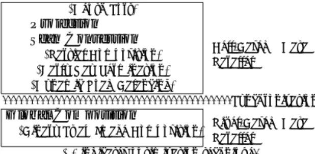
(2) we assume the cell to be a tetrahydra. ( 1 ) Projection Phase: Project a given threedimensional data(cell) into a two-dimensional screen and find the projection area(R) for each data(cell). ( 2 ) Scan Conversion Phase: Perform scan conversion for each projected cell. More precisely, for each pixel P (x, y) in the projection area(R) on the screen, calculate the cell’s contribution (color(RGB) and opacity(α)) to pixel P (x, y) and depth values (zf rontandzback ) for both the front and back intersection points where the ray corresponding to pixel P (x, y) intersects the cell. In the rest of this paper, we refer to the data structure consisting of these four parameters (RGB, α, zf ront andzback ) as ray segment. As the result of the scan conversion of a cell, ray segments for each pixel in the projection area(R) are computed. For every cell, compute the ray segments. After that, for each pixel on the screen, gather the ray-segments corresponding to the pixel and make a depthsorted list of these ray segments (Figure 2). ( 3 ) Composition Phase: Given the raysegment lists for all pixels on the screen, calculate the pixel value(color) by compositing the depth-sorted ray segments in the ray-segment list from front to back by alpha blending using Porter-Duff’s over operation5) . Now, we finally obtain the volume rendered image. Here, we have to note that, even in the scan conversion phase, one may perform composition of the neighboring ray segments in the ray-segment list for a ray if these two ray-segments are derived from the neighboring cells contacting each other along the ray. We refer to this composition in the scan conversion phase as partial composition6) (Figure 3). The resultant of the partial composition of two ray segments is again a ray segment. If we can apply partial composition successfully when a new ray-segment is inserted into the ray-segment list, we can reduce the length of the ray-segment list and list manipulation overhead due to the length of the list. Moreover, the opacity of a partially composed ray segment is higher than the opacity of each ray segment used in this partial composition. This feature greatly helps us to develop the optimization scheme. 2. scan convert. 1. project. 3. composite. 図1. Cell Projection. NULL 図 2 Ray-Segment List. Partial Composition. Partial Composition. 図 3 Partial Composition. described below.. 3. Parallel Implementation 3.1 Fundamental Implementation As we have mentioned before, the goal of our research is volume visualization of simulation results on a PC cluster. So, without a lack of generality, we can assume that the unstructured volume data has already been distributed among the nodes of the PC cluster. However, we have to remenber that the best data distribution pattern for the simulation may not be the best pattern for the visualization. This is the starting point of our parallel volume rendering(PVR) implementation. In the following discussion, we assume the system has N working nodes(WNs) for computation and one control node(CN) for global management of the load distribution and user interface including final image output. Once the data(cell) has been generated and distributed among the working nodes (WNs), the computation for the projection and scan conversion phases can easily be parallelized since there is no essential dependency between these computations. −46− 2.

(3) (Depth Sort). Projection Scan Conversion. Cell-Based Data (Partial Composition) Parallel (Early Ray Termination) (Dynamic Load Balancing) . . . . . . . . . . . . . . . . . . . . . . . . . . . . . . . . . . . . . . . . . . . Synchronization. Global Composition. Pixel-Based Data Parallel ( ) indicates optimization technique.. (Binary Swap Image Composition). 図 4 Parallel Implementation. for each cell. So, as the first step, each WN performs the projection and scan conversion of the cells which are assigned to the WN and generates its own ray-segment lists. When all WNs complete this computation, the composition phase starts as the second step. Now, we can utilize the pixel-level parallelism, so we assign the computation for a certain region of the screen to each WN and perform the parallel composition as follows. For each pixel in the assigned region, each node 1)gathers from other nodes the raysegment lists corresponding to the pixel, 2)merges them into a single depth-sorted ray-segment list, and then 3)calculates the pixel value(color) by compositing the depth-sorted ray segments in the raysegment list from front to back by alpha blending using Porter-Duff’s over operation5) . Now, each node finally obtains the volume rendered image for its own region. Then, each WN sends its image to the control node to output the overall volume rendered image onto the display. Though we cannot explain the detailed implementation of the global composition phase due to the page limit of this paper, we have adopted the Binary-Swap Image Composition(BSC) scheme7) to reduce both the communication overhead and the load imbalance. We also refer to this composition phase as the final composition phase or global composition phase if we need to distinguish it from the partial(local) composition in the scan conversion phase. Our fundamental parallel implementation itself is quite simple. The most important feature of our fundamental implementation is that it aggressively applies the partial composition in the scan conversion phase so that it can reduce the data size of each ray-segment list required for exchange in the final composition phase. The previous work by Ma, et al.4) proposed the parallel implementation which executes both the scan conversion and (global) composition processes. concurrently. Matsui, et al.8) have also adopted a similar technique for their structured-grid parallel volume rendering system. We also considered adopting this idea. But our conclusion has been negative so far, because 1)it may incur the problem of frequent asynchronous interprocessor communication, 2)our partial composition scheme may reduce the cost of global composition and also it can be thought of as a concurrent execution of the projection phase and the composition phase, and furthermore, 3)we are currently developing a technique like pipelining which may hide the cost(latency) of the global composition in some other work. 3.2 Optimizations 3.2.1 Approximate Depth Sorting By adopting partial composition, if the program could process the scan conversion of the cells in depth-sorted order, it could reduce the length of the ray-segment list, and thus it could reduce the list manipulation cost at the same time. So we have introduced an approximate depth sorting before the projection phase. 3.2.2 Early Ray Termination Erly ray termination(ERT)9) is an optimization technique which neglects the rendering of invisible or less contributed object (voxel, cell, and so on). Therefore, the ERT contribute too much to the reduction of the volume rendering cost, though its effect depends on the opacity of each object6) . Since ERT is a pixel-based optimization technique, it is easily implemented in the composition phase of our algorithm. However, the most time-consuming process in cell-projection parallel volume rendering(CP-PVR) is the scan conversion time. For this purpose, we have proposed an ERT technique which we call conservative early ray termination10),11) and implemented it into the Scan Conversion phase.. 4. Dynamic Load Balancing 4.1 Load Imbalance in CP PVR In this section, we first discuss the three major sources of load imbalance in our CP PVR program. 1. Load imbalance due to initial data distribution: As we have mentioned before, the goal of our research is volume visualization of simulation results on a PC cluster. In this case, the best data distribution pattern for the simulation may not be the best pattern for the. −47− 3.

(4) visualization. 2. Load imbalance due to view dependency of scan conversion time: The scan conversion time of each cell is proportional to the size of its projected area; thus, it may vary according to the viewpoint. This is what we call the view dependency of scan conversion time. 3. Load imbalance due to run-time feature of ERT : The effect of ERT strongly depends on the opacity of each cell and the viewing direction. Both the opacity and viewing direction are the fundamental parameters for volume visualization, and they frequently change during the visualization. Thus, it is impossible to estimate the effect on the computation of ERT in advance. Because of the irregularity of the unstructured volume data, static load distribution such as regional partitioning (3D-block cyclic8) , and so on) does not help too much. The simple static load distribution scheme which distributes an equal number of cells to each WN may reduce the degree of imbalance, but it cannot solve the second and third sources of load imbalance. The first two sources of load imbalance can be solved by preprocessing once a viewpoint is given. Previous work4),12) adopted such a preprocessing based load balancing scheme. In this scheme, researchers performed data redistribution as a preprocessing phase, taking the effect of view dependency into account. But, it cannot deal with the third source of load imbalance. Furthermore, it is hard to keep track of the quick movement of the viewpoint. In order to solve these three sources of load imbalance, we chose the distributed work-stealing scheme as the dynamic load balancing(DLB) scheme for postprocessing. In this scheme, when a working node(WN) completes the scan conversion of its own cells, it receives the cells from another WN which still has cells to be processed. Due to the dynamic behavior of this scheme, it can easily deal with the dynamic feature of the ERT effect. 4.2 Work Stealing As we mentioned in Section 3, our CP PVR program is composed of two different kinds of data parallel regions(Figure 4). According to our preliminary study10) , we find that the first region which utilizes cell-based data parallelism is quite dominant in the overall performance. We also find that the second region (global composition phase). is rather static compared to the first region, and the cost of data migration to implement DLB is relatively high in the second region. Therefore, we apply the DLB scheme only to the cell-based parallel region, while the static load balancing scheme is applied to the pixel-based parallel region. (1)Amount of Data(cells) To Be Migrated At a Time. In order to implement the DLB scheme for a PC cluster system, it is mandatory to lessen the frequency of data migration. Furthermore, the total of the data migration cost and the cost required to process the migrated data should be comparable to, or smaller than, the cost required to process the remainding data after migration. Therefore, the amount of data to be migrated at at time should be adapted according to the amount of remainding data. For this to be achievable, we chose a data size based on a somewhat guided self-scheduling. At the time of migration, 1/x of the remaining cells are sent to the idle WN on request. Currently, we have chosen 3 as x, based on the preliminary experimental results. (2)Node Selection Policy For the simplicity of implementation, our current DLB scheme relies on the CN to maintain the information required to make decisions on the source node of data migration. And inter-node communication to gather any DLB-related implementation is performed with polling-based asynchronous messages, where each node weak-periodically checks the arrival of messages. The following three policies have already been implemented as a node selection policy. Random Scheme : The CN maintains the list of busy WNs above a certain threshold which have remaining cells to be processed. When the CN receives requests for data migration from an idle WN, it chooses a busy WN at random from the list of busy WNs and informs the idle WN about the selected WN. Max-Remain Scheme: The CN maintains the list of busy WNs, as in the random scheme. But the CN also corrects the information about the amount of remaining cells on each of the busy WNs. When the CN receives requests for data migration from an idle WN, it chooses the WN which may have the biggest work to do from the list of busy WNs and informs the idle WN about the selected WN. Bounding Box Scheme: This scheme utilizes geometric information in order to find busy WNs. In. 4 −48−.

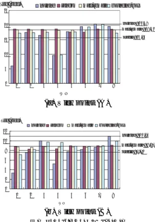
(5) Tsc (sec). random. nothing. max-remain bounding-box. 25 nothing : 20.38 max-remain : 18.40. 20. oracle : 15.85. 15. 10. 図 5 Sample Data (Human Aorta). 5. 0. 1. 2. 3. 4. 5. 6. 7. 8. WN. (a) Viewpoint (A) (a)Viewpoint(A). (b)Viewpoint(B). Tsc (sec) nothing. 図 6 Bounding Box Representations of Initial Cell Assignment Viewed from Two Orthogonal View Directions.. random. max-remain. bounding-box. 12. nothing : 10.93. 10 max-remain : 8.87. this scheme, each WN first computes the bounding box for all cells inside the node. This can be done simultaneously at an approximate depth-sorting time without paying any cost. Once the bounding box on each node is computed, WNs inform the CN of their bounding box information. When the CN receives requests for data migration from an idle WN, it chooses the WN whose bounding box overlaps the idle WN’s bounding box and informs the idle WN about the selected WN. This scheme is proposed in antcipation of the increase of the possibility of partial composition. We may possibly implement this scheme without any intervention of the CN if all WNs share their bounding box information.. 5. Evaluation In this section, we evaluate the effect of the dynamic load balancing schemes. For a relatively large sample of volume data, we used segmented human aorta simulation data(Figure 5). This dataset consists of 307,565 unstructured cells of tetrahydra, with 62,475 vertices in total. Figure 6 shows bounding box representations of the initial cell assignment viewed from two orthogonal view directions, (A) and (B). The rectangular boxes in these figures represent the bounding-box of each WN. A almost equal number of cells are assigned to each WN initially. An 8nodes PC cluster(Pentium4 3GHz, 1GbE) for WNs and a 1-node PC(Pentium4 2GHz, 1GbE) for the CN are used in our experiment. Figure 7 shows how our DLB schemes improve the load imbalance in the scan conversion phase with ERT. The y-axis of this figure indicates the. 8. oracle : 7.70. 6 4 2 0. 1. 2. 3. 4 WN. 5. 6. 7. 8. (b) Viewpoint (B) 図7. Comparison of DLB Schemes. scan conversion time(Tsc) at each WN and the horizontal line labeled oracle indicates the arithmetic mean of the scan conversion time of each WN without applying DLB. From this figure, we can confirm the effect of DLB. We can also confirm that the max-remain scheme achieves the best performance for both two viewpoints in this environment. The bounding-box scheme was expected to perform the best for the viewpoint (B), however, Figure 7(b) doesn’t show such a result. It is because our current implementation of the bounding-box scheme doesn’t consider the load imbalance among WNs whose bounding boxes do not overlap each other, and thus it somewhat restricts the possibility of the load balancing. We think this problem can be solved by combining the bounding-box scheme and max-remain scheme. Table 1 summarizes the overall effects of the optmization techniques used in our CP-PVR program. ”Base” stands for the parallel processing without ERT and DLB. From this table, we can confirm the 2.86- and 4.32-times speedup compared to the ”Base” implementation for viewpoint (A) and (B), respectively.. 5 −49−.

(6) 表 1 Overall Effects Scan Conversion Time Tsc[sec] Optimization Level (A) (B) Base 45.37 25.48 ERT 20.47 10.93 ERT + DLB 18.40 8.87 ERT + DLB + ERTsharing 15.82 5.89 ERT:Early Ray Termination DLB:Dynamic Load Balancing. 6. Conclusion We have proposed a cell-projection parallel volume rendering system for simultaneous visualization of simulation results on a PC cluster. By adopting the early ray termination and dynamic load balancing optimization techniques, it could achieve a 4.32-times performance improvement in our experimental environment. We would like to further investigate the various features of our program in the near future.. 7. Acknowledgment We would like to thank Prof. T. Matsuzawa and Dr. M. Watanabe of JAIST for providing the aorta dataset. Part of this research was supported by the Grant-in-Aid for Scientific Research (S)#16100001 and (B)#13480083 from JSPS.. 参. 考文. 献. 1) Mori, S., et al.: ReVolver/C40: A Scalable Parallel Computer for Volume Rendering – Design and Implementation–, IEICE Trans. Inf. & Syst., Vol.E86-D, No.10, pp.2006-2015, 2003. 2) Maruyama, Y., et al.: Parallel Volume Rendering with Commodity Graphics Hardware, IPSJ SIG Meeting(2003-ARC-154), Vol.2003, No.84, pp.61–66, Aug. (2003). 3) Max, N., et al.: Area and Volume Coherence for Efficient Visualization of 3D Scalar Functions, Computer Graphics (San Diego Workshop on Volume Visualization), Vol.24, No.5, pp.27–33 (1990). 4) Ma, K.-L. and Crockett, T. W.: Parallel visualization of large-scale aerodynamics calculations: A case study on the Cray T3E, IEEE Parallel Rendering Symposium, pp. 95– 104 (1997). 5) Porter, T. and Duff., T.: Compositing Digital Images, ACM Computer Graphics (SIGGRAPH ’84), Vol.18, No. 3, pp. 253-259 (1984).. −50− 6. 6) Lichtenbelt, B., et al.: Introduction to Volume Rendering, Hewlett-Packard Professional Books, Prentice Hall PTR, (1998). 7) Ma, K.-L., et al.: Parallel volume rendering using binary-swap compositing, IEEE Computer Graphics and Applications, Vol.14, No.4, pp.59–68 (1994). 8) Matsui, M., et al.: Reducing the Complexity of Parallel Volume Rendering by Propagating Accumulated Opacity, Technical Report of IEICE,Vol.103, No.249, pp.13–18(2003). 9) Levoy, M.: Efficient ray tracing of volume data, ACM Transactions on Graphics, Vol.9, No.3, pp.245–261(1990). 10) Takayama, M.: Dynamic Load Balancing on Parallel Visualization of Large Scale Unstructured Grid , Master’s Thesis, Graduate School of Informatics, Kyoto University, Feb. (2004). 11) Takayama, M., et al.: Cell-Projection Parallel Volume Rendering with Early Ray Termination, Visual Computing Symposium, June 2004(in printing). 12) Chen, L., et al.: Parallel performance optimization of large-scale unstructured data visualization for the earth simulator, Proc. of the Fourth Eurographics Workshop on Parallel Graphics and Visualization, Eurographics Association, pp. 133–140 (2002)..

(7)