A POLLING MODEL WITH RETRIAL CUSTOMERS

Journal of the Operations Research Society of Japan

Vol. 40, No. 4, December 1997

A POLLING MODEL WITH RETRIAL CUSTOMERS

Christos Langaris University of Ioannina

(Received July 31, 1996; Final June 4, 1997)

Abstract A polling model with n stations and switchover times is considered. The customers are of n different types, arrive t o the system according t o the Poisson distribution in batches of random size, and if they find the server unavailable, they start to make retrials until succeed to find a position for service. Each batch may contain customers of different types while the numbers of customers belonging to each type in a batch are distributed according t o a multivariate general distribution. The server, upon polling a station, stays there for an exponential period of time and if a customer asks for service before this time expires, the customer is served and a new "stay period" begins. Finally the service times and the switchover times are both arbitrarily distributed with different distributions for the different stations.

For such a model we obtain formulas for the expected number of retrial customers in each station in a steady state. Our results can be easily adapted to hold for zero switchover times and also in the case of the ordinary exhaustive service polling model with (without) switchover times and correlated batch arrivals. In all cases mentioned above (retrial model, exhaustive model, switchover times, zero switchover times) to find the expected queue lengths we need finally to solve a set of only n linear equations ( 0 ( n 3 ) arithmetic operations to compute the coefficients).

Tables of numerical values are finally obtained and used t o observe the system performance when we vary the values of the parameters.

1. Introduction

A polling model is a system of n queueing stations accessed by a single server in a prescribed order. This kind of systems has been proved useful particularly to model maintenance processes, multiprocessor computers, communication networks and manufacturing systems. There are many varietes of polling models depending on the service disciplines (exhaustive, gated, limited etc.), the existence or not of swit chover times between stations, the capacity of the buffers, the order in which the server polls the stations etc. For a complete survey on the earliest works in polling systems see Takagi [26]. More recently we have to mention the works of Resing [22], Eisenberg [8], Srinivasan et a1 [24] and Altman & Yechiali [2].

As far as we know, in all studies of polling models appeared till now in the literature the customers are assumed to form, upon arrival, a queue in each station and t o wait there until the server selects them for service. Thus the customer in such a model does not have the chance- when he finds, upon arrival, the server busy in one of the stations, or performing a switchover time - t o leave the system and to retry individually for service later.

Queueing systems with retrial customers have received considerable a t tention recently and are widely used in computer and communication networks and in telephone switching systems. They are characterized by the fact that an arriving customer, who finds the server busy, leaves the system and repeats his demand after a ra,ndom amount of time. A complete description of situations where such queues arise, and extensive reviews of the earliest work on the subject may be found in Yang & Templeton [27] and in Falin [g]. We have also to mention here the works of Kulkarni & Choi [17], Falin & Fricker [10], Grishechkin [14], Falin, Artalejo & Martin [ l l ] , Langaris & Moutzoukis [18], Moutzoukis & Langaris [21]. Both kind of models - polling models and systems with retrial customers - have been

used separately to model complex situations particularly in communication networks. Thus in the field of Local Area Networks (LANs) one can find a number of models handled as polling systems with queued up customers (Bux [6], Ferguson & Aminetzah [12], Fournier

fc

Rosberg [13], Borst [4]), while in the same area, various models with specific protocols have been discribed and analysed as retrial systems with a single station ( Kulkarni [16], Choi. Shin & Ahn [?l).

In the work here. we have tried to combine these two characteristics. and to study a polling model with retrial customers. Thus in the model considered, there are n types of customers (one for each station) arriving in batches of random size ( a batch may contain customers of all types) and making retrials in each station until they find t,he server available. There is only one server who polls the stations in a cyclic order and stays in each one of them for a random amount of time awaiting for customers seeking service. There is finally a switchover time when the server passes from a station to the next. For this model, we will describe a method to obtain the mean number of retrial customers in each sta,tion (and the mean waiting time, through Little's formula, consequently).

An interesting feature of the approach used is that we. can obta,in immediat'ely the corresponding quantities (queue length, waiting time) in the case of zero switchover times, simply by replacing in the obta,ined final formulas, the mean and the second moment of the switchover time by zero. Moreover by sending the mean retrial time and in the sequel the mean "stay period" to zero we a,rrive a.t the corresponding formulae of the ordinary exhaustive service polling model with or without, switchover times and correhted batch arrivals.

The mean queue lengths (waiting times), in all models described above are found, by solving finally a set of only n linear equations, while the number of arithmetic operations required to derive the coefficients of these equations is O(n3) or less. Note that,, for the exhaustive (and gated) polling model with swit chover times and single independent arrivals, Sarkar & Zangwill [23] derived (using the concept of "system time") the expected waiting times, by solving a set of n linear equations (for the variances of the cycle times) too. The mean waiting time in the corresponding model with correlated batch arrivals has been obtained in Levy & Sidi [l91 as a solution of a set of n3 linear equations while Boxma [S] derived for the same model a pseudoc~onservation law for t h e mean waiting times.

The paper is organised as follows. After the full description of the model in Section 2,

a system of equations satisfied by the steady state probabilities are obtained in Sect'ion 3. In Section 4 these equations are used to derive expressions for the mean number of retrial customers in ea,ch station. The case of the exhaustive service polling model with correla,ted batch arrivals is investigated in Section 5. Finally in Section 6 numerical results are obtained for the retrial model and used to observe the system performance under changes in the values of the parameters.

2. The Model

Consider a system consisting of n infinite capacity queueing stations S; i = l , 2, .

..,

n ar- ranged in a cyclic order. There is only one server who visits the stations in a prescribed cyclic order Sl, S2, . ..

,

Sn, Si, Sy,

...

Customers arrive into the system according t o the Poisson distribution with parameter A in batches of random size. Each batch may contain customers of different types

Pi

i =

l , 2 ,

...,

n and a

Pi

customer asks always for service at the Si station. If we denote by X{

A Polling Model with Retrial Customers 4 9 1

where in general X = (xi, .r2, . . . , a ' ^ ) and zx = Z ; ~ < ~ . . . Z : ~ .

If an arriving batch of customers finds the server in the Sz st'ation and idle then one of the P, customers of the batch (if any) commences service immediately and the remaining

c,

customers j = 1,2, . .

.,

n join the retrial group of the

6,

station respectively and seek for service individually after an exponentially distributed (parameter for the

,5',

station) amount of time.

If an arriving batch finds the server either busy in one of the stations or performing a switchover time then all customers of the batch join the corresponding retrial groups.

The server upon polling a station stays there for a n exponential amount of time (pa- rameter a, for the

6,

station). If a customer arrives (either from. outside or from the retrial group) before this time expires then the customer is served and afterwords a new exponen- tial "stay period'' begins. When for the first time the "stay period" ends before an arrival occurs, the server switches t o the next station. A switch from one station to another always requires a switchover time.

The service time of a customer in the ,Si station is distributed according t o an arbitrary distribution with distribution function (D.F) Udx), probability density function (p.d.f.)

u ; ' ( x ) with finite mean Gi and second moment G $ while the server switchover time between

the (i - a,nd ith station is assumed to be also arbitrarily distributed with D.F.

wx),

p.d.f. vi(x) and finite mean 6; and second moment for all i = 1 , 2 , . . .

,

n. All the processes defined a,bove are assumed to be independent t o each other.

3. S y s t e m State A n a l y s i s

We will start our analysis by considering firstly a more general model with arbitrarily dis- tributed "stay periods" instead of the exponential ones. Thus we assume that the "stay period" of the server in station

'5';'

i = l , 2,

...,

n follows a general distribution with p.d.f. 0;' ( t ) , D.F. B, ( t ) and finite mean h,.

Let now L? ( t ) be the number of customers in the retrial group of station S;' (the one in service-if any- is not included) at time t , and

Define

if the server is working in

Si

a t t

W =

if the server is staying idle in Si a,t t

if the server is switching from t o S;' at t , and let

pi(k, X , t)dx = Pr([(t) = là L ( < ) = k , z

<

c ( t )

5 x

+

dx)

where U;'(t), B i ( t ) , Vi(t) are at t , the ela,psed service time, the ela,psed "sta,y period" and the elapsed switchover time respectively. It is easy t o see that for X

>

0 and for all i = 1,2, . . . n

k

~ . ( k , X

+

dx, t

+

dx) = (1 - Adx - C,[x)dx)p;'(k, X, t)

+

Adx _{g ( k} - m)pi(rn, X , t ) m=0

k*

+

Adx ^(m;)qi(k - mI,x,t)

k

d i ( k , X

+

d x ,

t

+

d x ) = ( l - Adx - i ; i ( ~ ) d ~ ) d i ( k , X , t )

+

Adx g ( k - m ) d i ( m , X , t ) , m=0

where we use m: = ( m l ,

...,

mi_l,O,

...,

mn) and for any ~ . d . f . f ( t ) with D.F. ~ ( t ) we / ( O

denote by

j(t)

the age-specific failure rate i.e. f ( t ) =

m

.

For X = 0 finally

where we denote by 1; the n dimensional null row vector with a unit in the ith position and of course if i = 1 then z - 1 = n.

R e m a r k : If we put v i ( x ) = V i ( x ) where is Kronecker's delta, in (3.4) and replace the second integral of the right hand side (which becomes now d i ( k , 0 , t ) ) with the integral in (3.5), then it is easy to see that the first two relations in (3.2), relation (3.3) and the new relation (3.4) describe in fact the model with zero switchover times. Note that in this case the probability d i ( k , 0 , t ) in (3.5) corresponds to the point in time at which the server polls station z.

Assuming now that a, steady state exists and defining

CO P ; ( z , X ) =

E

lirn pi(k, X , t ) z k k=O t+OO 00 Q ~ ( z , X ) =

E

lim q i ( k , X , t ) z k k=O t+OO 0 0 Di ( z , X ) =

E

lim cli ( k , X , t ) z k , k=O t-OO we obtain from (3.2)

A Polling Model with Retrial Customers 493 while to handle equation (3.7) we have to consider (Gross & Harris [15],p.1 15 ) the system

By solving this system in the usual way, we arrive at

where U and V are constants. The general solution of (3.7) is now of the form V = F ( U )

and so by putting x = 0 in the above equation we obtain the unknown function F as F (W) =

Qi((%

...,

&-l, W , %+l,

...,

Zn\

0). Thus finally

To find now the unknown quantities in (3.9), (3.10) and (3.12) we will use the boundary conditions (3.3)- (3.5). Let us define

Then from (3.3) by forming the generating functions we obtain after manipulations

while from (3.4)) using (3.9) and (3.10)

(3.15) pi(z,O)~;(A - AG(z))

+

Di(z,O)<(A - AG(2)) = Qi(z,O),

with U * ( - ) , v,;(-) the Laplace transforms (L.T) of U , - ( - ) , vi(-) respectively. Finally from (3.5)

Let us consider now the generating function

Q,

(2). By s~bstit~uting Qi(z, X) from (3.12)

to (3.13) and evaluate the integral we arrive at

with b * ( - ) the L.T. of bi(-). In a similar manner (using (3.12) again)

00

(3.18) Qi(z, x)hi(x)dx = bz(A - AG(z;)

+

kipi)q;(k, O)zk .

k=0

Substituting fina,lly Qi(z, 0) and Pi(z7 0) from (:3.19) and (3.14) to (3.1.5) a,nd using (3.16), we arrive at

A Modified Model: Let us consider now a different "staying" policy in which the server is not allowed to repeat, t,he "stay period" each time a customer ~omplet~es service but, now the total time he is allowed to spend in an idle mode, from the instant he polls the station until the instant, he leaves it, is an arl~itrarily distributed rev. with p.d.f bi(t) and D.F. Bi(t) for the iih station respectively. In this case, let us replace the first and second of (3.1) by

where now Bl(t) is the total time the server alrea,dy spent in an idle mode before commencing his more recent service and z y ( t ) is the elapsed "stay period" counting from the last epoch the server becomes idle. If now we repeak the previous analysis t,hen, for :c

>

0, we obtain

while from the bo~mdary conditions

aQ{(z) + A G(z) - G(z:) -

pi- Q:(z) = P:(z7 0)

l?& zi

(3.22)

with Q:(z) E If now we write for Q (z)

and

JF

JF

Qi(z, y, x)bi(x

+

~ ) d x d ~ expressions similar to (3.17) and (3.18) we arrive again, a,fter manipulations, at the basic relation (3.20) (with ~ { ( z ) , D!(z, 0) instea,d of Qi(z), D.(z, 0) respectively).

Note here that, from the second and third of (3.22)

which is (3.15). Comparing (3.21), (3.22) wit h the corresponding relations in the original model, one realizes that the differences between the two models lie in fact in the formulae giving Qi(z, y

,

X ) D:(z, 0), where the term

L.

(y

+

-) does not allow a simple integration with respect to y . It is now cleax that if we assume exponential "stay periods" then this term becomes a constant, and, as it is expected, the two models become completely equivalent.

A Pollins Adodel with Retrial Cu.~tomers 495

Exponential exponent ia1 ') stay

stay periods: Let us assume now that bi(t) = aie-a2t i.e. we assume periods". In this case from (3.9) and (3.10) we obtain

while from the boundary conditions (3.14)) (3.16) we get

(3.26) Di(z, 0) = ai-lQi-l(z).

Substituting finally from (3.26) to (3.20) we arrive) for all i = l , 2,

...,

n, a t

Note t h a t ) as one can see from (3.21)) (3.221, relations (3.23)-(3.27) are also satisfied by

P/(z), Q;(Z)) D;(Z)) where P;(Z)

=

JF

JF

P:(z, y) x)dydx.

Note also that by putting U:(-) = l in (3.23)-(3.27) we obtain immediately the corre- sponding formulae for the model with zero switchover times.

4. Mean Queue We will try here to station for the case

Lengths in steady state

derive expressions for the expected number of retrial customers in each of exponential "stay periods".

Before starting our analysis we will obtain a necessary condition for the stability (bound- edness in probability of the total amount of work in the system a t any time t ) of our model. Let us define

'n,

then

Theorern 4.1 A necessa,ry conclition for stability is

ProoE The proof follows the steps of that in Theorem 3.1 in A l t ~ n a n & Levy [3]. Suppose that our system is stable and p

2

l . Consider? as an alternative system (System 0)) the ordinary exhaustive service polling model without switchover periods. System 0 is a system with greedy (the server never idles at a nonempty queue) and exhaustive service policy and one can ea,sily understand (see Liu & Nain [20] ) tha,t a t every moment t the a m o ~ ~ n t of unfinished work at this system is less than or equal to that of our original retrial model. Moreover it is known (see for example Altman et a1 [l] ) that a necessary (and sufficient) conclition for the stability of System 0 is p

<

1. Thus) for p

2

l , the amount of work in Systeni 0 converges in distribution to infinity and this is true consequently for our original retrial model too. It contradicts of course to the hypothesis that the retrial model is sta,ble? and this proves the t l ~ e o r e ~ n .

From here on a,nd all throngh the following sections we will assume p< l. We continue the analysis proving the following lemma.

Lemma 4. l The generating functions pi(z), Qi(z),

Di

(z) at the point z = l are given by

Qi(1) = l - P l

ui (Gm

+

G )

Proofi We will prove the lemma under more general assumptions on the system char- acteristics using arguments similar to that used in section 5 of Altman et a1 [l].

Let us consider the more general model with arbitrary stationary: total stay periods, switchover times, interarrival times with batch arrival rate A (gi is the mean number of

Pi

customers per arrival) and service times with mean iii for the ith queue. Suppose also that the workload is stationary and that the model admits a steady state.

Let finally

... <

T-l

<

To

5

0

< Tl

<

T2

<

...

be the time epoches the server arrives at queue l , N(t) the point process that counts the number of these arrivals until time t, P O the Palm probability related to AT, EO the expectation with respect to (w.r.t.) PO, v

>

0 the intensity of N(t) and Cn =

Tn+l

-

Tn

the nth cycle time. We assume that the cycle times are stationary and ECo

<

m.

The slope of the workload

W k ( t )

in queue k ats time t is equal to -1 if the server is working in queue

k

att t and equal to 0 in all other cases. 'Thus using Miyazawa's rate conservation principle and observing that the mean magnitude of the jump of VVk(t) is gkiik, we realize that

~ ~ ( 1 ) = P ( t ( 0 ) li) =-EW:(O) Agiiii,

where [(t) has been defined in page 3 and W:(-) means the right derivativeof

W i

(m). Thus

(4. l) holds.

Define now the sequences

{oil,

{yk}, { b i } m = 0, l , 2,

...

where

ok,

7& is the time spent by the server at the mth visit to queue i, in a busy mode and in an idle mode respectively and 6; is the switchover time between ( i - 1Ith and ith queue (at the mth visit to queue i ) .

Following the steps of Proposition 5.2 in Altman et a1 [l] we arrive easily at

(4s4) ~ ~ ( 1 ) = P([(O) = vi) = V E O ~ ;

But the cycle time CO can be written as CO = ~ : = ~ ( o ;

+

y;

+

6;) and as vE°C = l we obtain

Using (4.4) and (4.5) we arrive, in the case of our original retrial model, at (4.21, (4.3) and the lemma has been proved.

Define now, for all i = l, 2,

...,

n

where Lai represents the number of retrial customers in station j (in a steady state) and [ = lim [(t) is defined in page 3. Let also Rij = Agj(1

+-

uiGi

+

Aiiiri) with ri = ( l - G(1:)).

t+m

A Polling ,Vodcl with Retrial Cu.~tome~$ 497

Theoreh1 4.2 The mean numbers of retrial custon~ers L:', i , j = l , 2,

...,

n are given

where Q l ( l ) is known from (4.2).

ProofiBy putting z = l in (3.27) we obtain a i Q i ( 1 ) ~ i - l ~ i - , ( l ) or

while from (3.23), it is easy to see that

(4.10) ~ ~ ( 1 ) = GiPi(17 0 ) , i = 1,2

,...,

n.

Then from (3.25) using (4.10) we obtain

Using finally (4.1),(4.2) in (4.11) we arrive at (4.6) easily.

Differentiating now relation (3.27) w.r.t. zj ( j

#

i ) at the point z = l we obtain

i , j = 1 , 2

,...,

n,

_i

_{# j .} and so by putting j - /c instead of i in (4.12) we arrive at

aj-k-1 Q.j-k-l I Qj-k + ~ ~ R j - ~ j -

(4.13) = -

_4.

+

_{~ ( A g ~ ~ j - k G j - k L j - ~}

aj-k aj-k aj-k Q l ( 1 ) ) -

Putting k = -l in the above relation we obtain (4.7) for

i

= j

+

l . Putting k = -2? and

using (4.7) with z = j

+

l , we obtain (4.7) for

i

= j

+

2. It is clear now that we can obtain,

in the same way, relation (4.7) for all i , j = l , 2 ,

...,

n , i

#

j.

To derive finally relation (4.8) we will use (3.26) and (3.24). Thus from (3.26)

and it is easy to see that

To finish our analysis we have to evaluate L:

=v

lzz1

. From (3.251,

where (4.15)

By taking now derivatives in (3.23) w.r. t

.

z j a t z = l and using (4.10) and (4.1) we finally

arrive at, (4.16)

where L$' =

lzz1

.

Thus t o evaluate L? we need the n2 quantities L:' for all

i , j = 1 , 2 ,

...,

n. We will try t o find them in the sequel.

Differentiating relation (3.27) twice w.r.t. zi a t z = l we arrive at

(4.17) [2pi ( l - pi)

+

a;] L!' - a . L$'-' = HI ( i ) , i = 1 , 2

,...,

n , with

while by differentiating (3.27) twice w.r.t. z j ( j

#

i ) a t z = l we obtain

with

If now we put j - k instead of i in (4.19) we obtain

Summing the above equations for all k and adding the result in (4.17) we arrive, for all

i = 1 , 2

,...,

n , a t

which are the first equations in the n2 unknowns L::. To derive the remaining ( n - 1 ) n equations we will use again relation (3.27). DifFerentiating twice (3.27) w.r.t. zi and z j ( i

#

j ) we get

A Polling Model with Retrial Customers

with

i , j , k = l

,...,

n

(4.25) -

pi\gfii~$

- pi\gtiii~Qj'

+

U~L" Jk -

~ ~ - ~ ~ y i - ~

= H4(i, j, k),

w i # k

Summing the above relations for a,ll r and adding the result in (4.23) we arrive at

with

~ 2 ,

Am 0 for any quantity Am. Equations (4.22) and (4.27) con~tit~ute a system of n2 equations from which the n2 unknowns L$ i, j = 1,2, . .

.,

n can be found.

From here on we will try to make the computations, required to derive LT, simpler, by reducing the number of equations in (4.22) and (4.27). Let us define

and consider the two sets of indices

A=

{(k, i ) : k = 1,2,

...,

in(?), i = l, 2,

...,

n},

=

{(k,

i ) : k =

B,

i = l., 2, ...,

B,

n even} where in(m) means the integer part of m.

where h!"^ z 0, _Am 0 for all i and for any quantity Am, and

Note here that the indices are moving in cyclic order, i.e. if for example n = 10, i = 1,

- - - (Gi-k) -

r = 3, k 5 then /L;-T E /L-2 /Ln-2 = /I&, Pi-k = ;"G, Ui-fe G6, hieT - hc'6),

Remark: For k = 1, one can easily see, that all sums in (4.29) are empty and so the quantities h?-) are, for k = 1 and all i, r , completely known. Using these quantities in (4.29) again, we get immediately the h(.,-) 'S for k = 2 and all i, r (each sum has now at most one, completely known, term ). continuing in the same way we obtain recursively the quantities h!-'-) for all k, i, r. Let us denote now the sums as

Then the sums, appeared in (4.30), have together no more than k (< in{:)) terms and, it is easy to see that, for all i , r , k

[i-(k-l), i]

;p(,,

r ) = 6;"-"(i, r )

+

hi-T 7 e%i, k) = 0

[(i-l), (i-l)-(k-l)]

^\,,

r ) = 6[kU1)(i - l , r - l )

+

hkl)-(T-l) ? ; p ( i , 0) = 0.

Thus when we pass from k - 1 to k in (4.29) we need in fact to perform only one addition (of two completely known, from the case k - 1, terms) to construct the new sum i^{i, r). Consequently, to calculate each h(-7-) in (4.29) we need to perform at most seven multiplica- tion/divisions and four additionisubtractions and so the number of arithmetic operations required to obtain all h(-,.) is O(n3) or less. Similar observations hold for h " where now the number of arithmetic operations is 0 ( n 2 ) or less.

Define finally L: FF

5

^p'

and i=1

then

A Polling Model with Retrial Customers 501

where the n quantities N j j = l , 2 ,

...,

n can be found as the solution of the system of linear equations

with i = 1 , 2 ,

...,

n and

n ei ei

6,

=

+

X

H 2 ( m , i ) )

+

X

X

h^.+k'').

Proof: Relation (4.31) can be obtained from (4.16) easily. Also from (4.22) Q , - Agi A 1

n

Lii - -Ni

+

-(Hi ( 2 )

+

Y,

Hi ( m , i ) ) ,

2^- i = 1 , 2 ,

...,

n

Pi m = l m#i

and substituting in (4.27) we arrive at

i , j = l , 2

,...,

n , _i

_#

_{j ,}

while from (4.27) by interchanging i and j and adding the obtained equation to (4.27) we get,

(4.35)

li,~zi

+

&Q,'

- \gi N~ - \g& = K . . 2 ~ 1 i = 1 , 2 ,

...,

n - 1

j =

i

+

l , z'

+

2,

...,

n. Equations (4.34) and (4.35) can be written (with j = i - 1 ) in a matrix form as

and so

or, by putting i

+

1 instead of i in the first

where the quantities h(-'-) are given by (4.29). Now it is clear that we can repeat the procedure using again (4.34) and (4.35) with j = i - 2, i - 3 ,

...

to obtain for all i = 1, 2,

...,

n ,

Using finally the above relations and the definition of

TVi

(the first of (4.28)) we arrive at the system of linear equations (4.32) a'nd the theorem has been proved.

5 . The case of exhaustive service

Let us suppose now thai pi

=

p , a; G a for all i = 1 , 2 ,

...,

n. If we assume that p ~r CO then

the ret,rial chara.cteristics of our model are swept out and the model becomes a.n exhaustive service polling system with "stay periods". If we assume in the sequel that a -+ oo then we get t,he ordinary polling model with exhaustive service, switchover times and correlated batch arrivals. We will try in the present section to obtain the mean queue lengths

q i

,

F',

L:

,

of this polling model with exhaustive service, as limits of the corresponding quantities

L^\ L?, L: of the retrial system, when ,u --+ m, a -+ CO. From (4.6), (4.7) it is easy to see that

lirn L?' = 0,

u-+m

lim ,uL" = Aqi - ~ ( 1 - p ) ~ ~ _n

P - + W

n+a

v

G m

Thus, as it is expected, for all i , j

Zyi

EE lirn lirn £7 = 0, a- p+oo while using (5.1) in (4.8) D,

w"

l - p

L,

= lirn lirn = -- a ~ > - o o p - + ~ ₂

+

i'iPi-lj- \ ^ G

If now we use (5.1) in (4.18), ( 4.20), (4.24) and (4.26), we obta,in the quantities

g . ( - )

=

lirn lirn H . ( - ) as

a+oo uÑ>-o

and from (4.28) the corresponding quantities, in the case of the exhaustive service model, are

By defining finally /^-l lirn lirn h,(->+) and taking limits in (4.29) we obtain, for all

UÑi-c p- .

A Polling Model with Retrial Customers

i - T

1 i-l

$G-k) - -

+

-iÑÑ(Aui9,

E

A'm7i) + pi

E

$;i-*)

2 - T 2-T

m=z-k+l m=%-r

i-r i-l

^ - k 7 i ) =

3.

1 - (m,;-k)

z - T 2%-k I - , , (pi-k

E

L,'";"

+

A<?iui-),

E

hi-, )

m=i-k+l m = z - T

where

p)

=

0,

m

Am E 0 for all i and for any quantity Am, and

r = O r = O

y.

=

23

,

dij = r = k

otherwise otherwise.

Note that the observation concerning the cyclic movement of the indices in (4.29) and the Remark following it hold for (5.5) too. Now we are ready to state the theorem

Theorem 5.1 For the exhaustive service polling model,

ZT

is given, for all j = 1,2,

. . .

,

n,

by

where the n quantities

N,

j = 1,2,

...

,

n can be found as the solution of the system of linear equations

with i = 1,2,

...,

n and

Relations (5.2) and (5.6) allow us to calculate the mean queue length in each station

for the exhaustive service polling model with switchover times and correlated

batch arrivals.

Note that, for this model with correlated batch arrivals, numerical calculations have shown that our results for the mean waiting time (excluding service)

coinside with the results obtained from Levy & Sidi [l91 formulae (n3 linear equations), while if we assume that G(z) = _A&/ Ai, then we get results for the model with single independent arrivals (A; the arrival ra,te in

P

station), i.e. the model of Ferguson &

Aminetzah [l21 (n2 linear equations), Sarkar & Zangwill [23] ( n linear equations), etc.

Remark: From the observation made in the end of Section 3 and the analysis in Section 4 it is easy to understand that to obtain the corresponding results for the retrial polling model with zero switchover times and correlated batch arrivals we have only to put 6; = = 0, in Lemma 4.1, Theorem 4.2 and in (4.18), (4.20), (4.24), (4.26) of Section 4.

In a similar way by putting f i = 6:) = 0 in Section 4 and assuming in the sequel

p+ m, a + ca we obtain results for the exhaustive service polling model with zero switchover times and correlated batch arrivals. In this case it is easy to see that the mean queue length in station j is given by

where the quantities

N',

satisfy again system (5.7),

h['.)

satisfy (5.5),

I\^,

are given by (5.4) and

with T 72. = AgjUi - 61,

(h

is Kronecker's delta). If finally we assume, in the above model,

single independent arrivals i.e. if we put above wij = gi,? = 0, \gi = A;, then numerical calculations have shown that our results for the mea,n waiting time (excluding service), in this case of zero switchover times, coinside with the results obtained from Ta,kagi[25].

Note that, in all models studied in the present work, to find the mean queue lengths one has to calculate first the quantities h!-'-) (O(n3) arithmetic operations), and in the sequel to solve a set of n linear equations ( O(n3) operations again). Thus the total complexity t o obtain the mean queue lenghts is finally O(n3).

6. Numerical results

The mean number of retrial customers in the jth station of the original retrial polling model

is given by

and from (4.6), (4.7), (4.8) and (4.31) it is completely known. To observe the way in which this mean value

L-,

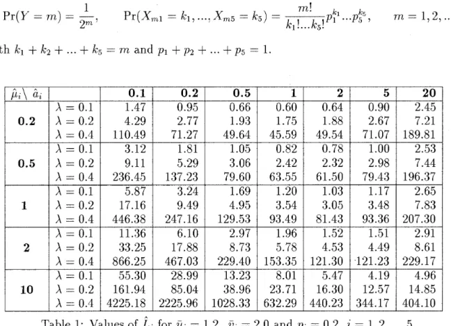
is affected when we vary the values of the parameters, we give here Tables

1 and 2. To construct the tables we assumed that n = 5, i.e. that we have a polling model with five stations, and that the service times and the switchover times follow exponential distributions,

A Polling Model with Retrial Customers 505 We a,ssume further that, if 1' denotes the batch size and Xmi i = l , 2, .

..,

5 the n u ~ n b e r of type i customers in a batch of size m, then

with k~

+

k-2

+

...

+

k5 = m and pi + p 2

+

... + p 5 = 1.

-

Table 1: Valuesof L; for i& = 1.2, 6; = 2.0 and pi = 0.2

Table 1 gives values of Li

(=L^

i = 1,2,

. .

.5) for the symmetric system (all parameters are statistically identical for all stations). We have used the symmetric system so as to have

a clearer picture of the way in which our models affected from changes in the mean stay period

hi

= I / a i , and in the mean retrial time

hi

= l / p i , particularly when the a,rrival rate A increases. In this table one can observe the large increase of L when we pa,ss from A = 0.1 to A = 0.2 a,nd particularly to A = 0.4, an increase which is more ampparent for large values of

,G,. Thus, for hi = 0.2 for example, L increases from 0.95 t o 71.27 when we pass from A = 0.1 to A = 0.4 in the case of ,hi = 0.2, while the corresponding values for

hi

= 10 are 28.99 and 2225.96. This means that in such kind of models, we should be careful with the permitted input. Sometimes, even small changes in the arrival rate, could increase dramatically the number of the retrial customers in the system.

An interesting phenomenon here is the behavior of L when we increase the mean stay period

&. It seems that, a t the beginning, when the mean stay period increa,ses it helps the

retrial customers t o find t,he server idle and t o start their service, which results of course t o a smaller

L.

This behavior continues until

&

becomes equal to a critical value. From this point and after any increa,se t o

a;

ceases to be useful1 for the system, on the contrary it prevent the server t o depart and t o start serving in the next station a,nd so L starts t o increase again and becomes large for large values of

2;.

Thus there is an optimal value,

a*.

say, of a;, a value with which we can achieve the minimal possible mean length L.

To observe in more details this optimal value of

a;

and the way in which it depends on the mean retrial time

fii

we present here Figures 1-4. In all figures we have used Mathematics

to plot L against

a;,

using for all i , A = 0.2, = 1.2, V i = 2.0 and pi = 0.2. In Fgr.1, where

with

Gi

= 0.5, = 1.66 and minL = 2.30, while in Fgr. 3 where the mean retrial time

A

increases to (i, = 2.0,

itl

= 3.2 and min L = 4.30. In Fgr.4 finally, {i, = 5.0 and we have

= 5.05, minL = 7.52. In all figures one observes a fast reduction of L, when

iii

increases

A

Figures 1-4: Plot of L for A = 0.2, iii = 1.2, = 2.0, pi = 0.2, i = 1,2,

...,

5.

Table 2: Values of for A = 0.4, = (0.2,0.2,0.5,1,2), ii = (0.2,0.2,0.5,0.5,1) and p = (0.05,0.1,0.15,0.3,0.4).

A Polling Model with Retrial Customers 507

froin small values to this optimal value

a*.

From this point and after, 1, starts to increase

again, but in a smoother way now. T h e general observation here is that the first thing that we have to do. if we operate a such kind of model, is to discover numerically this optimal 6"

and to arrange the mean time we will allow the server to stay in each station, accordingly. Table 2, finally, represents values of

L,

z = 1 , 2 ,

...,

5 for an asymmetric system now. with A = 0.4 and ,G = (0.2,0.2,0.5,1,2), 5 = (0.2,0.2,0.5,0.5, l ) , p = (0.05,0.1, 0.15,0.3,0.4), i.e.

a system with small values of t,he parameters for the first two and larger for the remaining three stations.

In t,his table one can observe the way in which t,he mean retrial lengths L, are affected from changes in the mean service times and in the mean switchover times v, (we have used the same value of i& and of for all stations). Thus, for = 0.5, L1 increases from 0.36 to 9.54 when we increase the mean service time from 0.2 to 1.2 while the corresponding values for the last station are

L5

= 4.03 and

L5

= 107.86 respectively. Similar observations hold for changes in the mean switchover times.

Acknowlegement

The author wishes to thank the Associate Editor and the two referees for their construc- tive comments which helped to improve the earlier version of the work.

References

[l] Altman, E., Konstantopoulos, P., Liu,

Z.,

Stabilit,~, inonotonicity and invariant quan- tities in general polling systems, Queueing Systems 11 (1992) 35-57.

21 Altman, E.. Yechiali, U., Polling in a closed network, Probability in the Engineering and Informational Sciences 8 (1994) 327-343.

3 Altman, E., Levy, H., Queueing in space, Adv. Appl. Prob. 26 (1994) 1095-1116. 41 Borst

,

S.C., Polling systems with multiple coupled servers, Queueing Systems 20 (1995)

369-393.

51 Boxrna, 0. J . , Workloads and waiting times in single-server systems wit h multiple customer classes, Queueing Systems 5 (1989) 185-214.

[G] Bux, W., Local area subnetworks: A performance comparison, IEEE Trans. Commun COM-29 (1981) 1465-1473.

[7] Choi, B.D., Shin, Y.W., Ahn, W.C., Retrial queues with collision arising from unslotted CSMA/CD protocol, Queueing Systems 11 (1992) 335-356.

8 Eisenberg, M., The polling system with a stopping server, Queueing Systems 18 (1994) 387-431.

[g] Falin, G., A survey of retrial queues, Queueing Systems 7 (1990) 127-168.

[l01 Falin, G., Fricker, C ; . , On the virtual waiting time in a M / G / l retrial queue, J . Appl. Prob. 28 (1991) 446-460.

[l11 Falin, G., Artalejo, J.R., Martin, M., On the single server retrial queue with priority customers, Queueing Systems 14 (1993) 439-455.

[l21 Ferguson, M., Aminetzah, Y

.,

Exact results for nonsymmetric token ring syst,ems, IEEE Trans, Commun. COM-33 (1985) 223-231.

[l31 Fournier, L., Rosberg, Z., Expected waiting times in polling systems under priority disciplines, Queueing Systems 9 (1991) 419-440.

[14] Grishechkin, S.A., Multiclass batch arrival retrial queues analyzed as branching pro- cesses wit 11 immigration, Queueing Systems 11 (1992) 395-418.

[l51 Gross, D., Harris, C., Fundamentals of Queuezng Theory, Wiley (1974), New York. [l61 Kulkarni, V.G., Expected waiting times in a multiclass batch arrival retrial queue, J.

Appl. Prob. 23 (1986) 144-154.

[l71 Kulkarni, V.G., Choi, B.D., Retrial queues with server subjedt to breakdowns and repairs, Queueing Systems 7 (1990) 191-208.

Langaris, C., Moutzoukis, E., A retrial queue with structured batch arrivals,priorities and server vacations, Queueing Systems 20 (1995) 341-368.

Levy, H., Sidi, M., Polling systems with correlated arrivals, IEEE INFOCOM'89 (1989) 907-913.

Liu, Z., Nain, P., On optimal polling policies, Queueing Systems 11 (1992) 59-83. Moutzoukis, E., Lalngaris, C., Non-preemptive priorities and vacations in a multiclass retrial queueing system, Commun. Statist .-Stochastic Models 12 (1996) 455-472. Resing, J . A.C., Polling systems and multitype branching processes, Queueing Systems

13 (1993) 409-426.

Sarkar, D., Zangwill, W., Expected waiting time for nonsymmetric cyclic queueing systems-Exact results and applications, Managament Science 35 (1989) 1463- 1474. Srinivasan, M., Niu S.C., Cooper, R., Relating polling models with zero and nonzero switchover times, Queueing Systems 19 (1995) 149-168.

Takagi, H., Analysis of Polling Systems, MIT Press (l986), Massachusetts.

Takagi, H., Queueing analysis of polling models: an update, in: Stochastic Analysis of Computer and Communications Systems, Elsevier Science-North Holland, (1990) 267-318.

Yang, T., Templeton, J.G.C., A survey on retrial queues, Queueing Systems 2 (1987) 201-233.

Christos LANGARIS

University of Ioannina, Dept of Mathematics 451 10, Ioannina. Greece