Dual structure in the conjugate analysis of curved exponential families (Statistical Inference of Records and Related Statistics)

202

Dual

structure in the

conjugate analysis

of

curved

exponential

families

統計数理研究所 大西 俊郎(Toshio Ohnishi) 柳本 武美(Takemi Yanagimoto)

The Instituteof Statistical Mathematics

Abstract

Curved exponential families$\mathrm{a}\mathrm{d}$ mitting conjugateplioldensitiesareintroduced

$\mathrm{a}\alpha \mathrm{l}\mathrm{d}$

exploreaIntx

0-ducingextendedversions of themeanand tlxe canonicalI) arameters,weexpandthe conjugateanalysis

to thesecurvedexponential families. Emphasis is puton dualstructures- In fact,we derive the dual

Pythagorean$1\mathrm{e}1\mathrm{a}\mathrm{t}\mathrm{i}\mathrm{o}\mathrm{r}1\mathrm{b}\backslash \ddagger 1\mathrm{i}\mathrm{p}_{\mathrm{b}}$ with resPectto posteriorrisks,each of which makes itclearhow the Bayes

estimator do minates other estim$\mathrm{l}\mathrm{a}\mathrm{t}\mathrm{o}\mathrm{r}\mathrm{b}\neg$. We also show that the conjugate prior density is the least

infor mative.

Key Words: closure under sampling, conjugacy, duality, leastinformation, Legendretransfozntatiott,

linearity, proper dispersion model. Pytllagolef.filrelationship,standgdized posterior mode

1. Introduction

Tlte conjugate analysis is

one

of the most $\mathrm{i}$mportant fields in Bayesian inference. It

has attracted interests of1rlany reseaxchers including Coiisonni alld Veronese (1992. 2001),

Guti\’errez-Pe\^ila $(1992, 1997)$ axld Guti\’erre?-Pefiaand Smith (1997). Si mplicity incalculating

the posterior mean, _{or the Bayes} estimator, is characteristic of $\mathrm{t}1_{1}\mathrm{e}$ conjugate analysis. A

minimaxproperty of the conjugate prior density

was

sbovv11$1_{\mathit{3}}\mathrm{y}$ Morris (1983) and Consomri

aIld Veronese (1992). Recently, _{extensions of}tlie conjugate prior density$1\mathrm{z}_{\dot{\mathrm{C}}}\iota \mathrm{v}\mathrm{e}$ beenstudied$1_{\lrcorner}\mathrm{y}$

$\mathrm{s}$uch authors

as

Ibrahim and Chen $(1998, 2000)$ and Yanagi moto and Ohnishi

$(200\overline{\mathrm{a}}\mathrm{a})$

.

Tlle

dual structure is elegantly observed iu the exponential fal1lilies and the curved exponential

$\mathrm{f}\mathrm{a}$ milies (Bariidorff-Nielsen $1^{\{}\mathrm{J}78\mathrm{a}$, Am ari

an

ld Nagaoka2000). $11\dot{1}$fact, the $\mathrm{i}$mportanceofthe cruvedexponential families

owes

largely to the dual structure. That in$\mathrm{t}$}$\mathrm{l}\mathrm{e}‘ \mathrm{j}\mathrm{O}\mathrm{l}\mathrm{l}\mathrm{j}\mathrm{u}\not\in\dot{\mathrm{i}}$ateanalysis was pursuedin naiveways byYanagimoto and Ohnishi $(\underline{?}0\mathrm{O}^{r}s\mathrm{a}\mathrm{b})$.

The originaldefinitionof conjugacy isclosure under

sa

mpling, i.e., that the prior andthe

posterior den ities belong to the

same

family of distributions, $\mathrm{w}\mathrm{h}\mathrm{i}\mathrm{c}1_{\mathrm{J}}$

was

defined by Raiffa and Schlaifer (1961, pp.43-57). Inthis paper

we

I1leaXl closure under sam$\mathrm{n}\mathrm{p}1\mathrm{i}_{1\mathrm{l}}\mathrm{g}$by $\mathrm{f}\cdot \mathrm{O}\mathrm{l}\mathrm{l}\mathrm{j}\mathrm{u}\mathrm{g}\mathrm{a}\mathrm{e}\mathrm{y}$

according to their definition. It is known that this definition produces am biguity. Take a

sam pling density in a naturalexponential family

$p(x;\eta)=\exp\{\eta x-\psi(\eta)\}a(x)$ (1.1)

for instance. The prior density $7\tau(\eta;m_{\dot{r}}\delta)$ cx $\exp[\overline{\delta}\{\tau\iota\iota r/-’\sqrt J(\eta)\}]b(\eta)$ is conjugate, that is,

closed under

sam

$\iota \mathrm{p}\mathrm{l}\mathrm{i}\mathrm{n}\mathrm{g}$, an$\iota \mathrm{d}$

we

cannot specify the tyPe of the supporting

measure

$b(\eta 1$ by

conjugacy alone. Diaconis andYlvisaker (1979) characterized thechoice$b(\eta)=1$ bylinearity

reasonwhy_{the present authors adopt such}

an

ambiguousdefinitionisaconjecture that closure under sampling in itself implies

a

$\mathrm{c}\mathrm{e}\mathrm{r}\mathrm{t}\mathrm{a}_{\int}\mathrm{i}11$opti

111U11Iproperty. This will be shownaffirmatively

inSection 3.

The conjugatc analysisisnotrestrictedtothenaturalexponential$\mathrm{f}\mathrm{a}\mathrm{m}$ ilycase. Mardia$\mathrm{a}\mathrm{r}$)$\kappa 1$

El-Atoum (1976) showedthat the von Mises distribution, which $\mathrm{i}\mathrm{t}\backslash$ inthecurved exponential

families,hasa conjugate priordensity. For the sampling density

$p_{\iota \mathrm{M}}(Xj \mu, \tau)=\frac{1}{2\pi I_{0}(\tau)}\exp\{\tau\cos(x-\mu)\}$, (1.2)

where $I_{0}(\tau)$ is the modified Bessel function of tlle first kind, the vonl Mises prior density

$P\mathrm{v}\mathrm{M}(\ell\iota;?n, \delta)$ isconjugate. $\mathrm{T}\mathrm{l}\dot{\mathrm{u}}\mathrm{f}\mathrm{i}$ prior densitywas enlplo

$.\mathrm{v}$ed by Guttorp andLockhart (1988)

and Rodrigues et al. (2000). $\mathrm{H}\mathrm{e}1^{\mathrm{n}}\mathrm{e}$ the linearityof tlie posterior

mean

of

$\mu$, does not hold in

the

sense

ofDiaconis and Ylvisaker (1979), although Rodrigues et $al$ (2000) pointedout that

atyPeoflinearity holds.

Thispaper hasthe$\mathrm{f}\mathrm{o}11\mathrm{o}\mathrm{w}\mathrm{i}\mathrm{n}_{\mathrm{p}\gamma}\mathrm{t}$)twoaim$1\mathrm{S}$

.

$\zeta)_{1\mathrm{z}\mathrm{e}}$istoreveal

an

essential aspectofthe conjugate

analysis. We considez the following$\mathrm{s}\mathrm{a}\iota \mathrm{x}\iota \mathrm{p}\mathrm{l}\mathrm{i}\mathrm{n}\mathrm{g}$density

$\mathrm{p}\{\mathrm{x};\mu$) $=\exp\{-d(x, \mu)\}a(x)\backslash$ (1.3) $\prime \mathrm{h}\cdot 1\mathrm{l}\mathrm{e}\mathrm{r}\mathrm{e}$

$x$ and $\mu$

are

$P$-dimensional, and $d(a, t)$ is$\mathrm{e}\mathrm{x}\mathrm{l}$)

$1^{\cdot}\mathrm{C}\mathrm{b}\mathrm{b}\mathrm{e}\mathrm{d}$ through th

le $(2p+2)$ functions,

$f_{k}(t)’ \mathrm{s}$and $l\iota\iota(t)$’s, as

$d(a, t)$$= \sum_{j=1}^{p+1}f\iota_{f}(a)\{f_{j}(t)-f_{j}’(a)\}$

.

In general, the density (1.3) belongs to the curved exponential families. As will be seen in

tl$\iota \mathrm{e}$subsequent sections, the$\mathrm{s}\mathrm{a}\mathrm{n}[perp] 1$)Iingdensity (3. $\cdot$

3) with$P$$=1$ covers the natural exponential

family (1.1) and the

von

Mises distribution (1.2). Thus,

a

unified discussion is possible. We

willslxov’ that the prior density of the for$\mathrm{m}\pi(\mu\cdot, m_{\backslash }.\mathrm{r})^{\backslash })$cx$\mathrm{e}\mathrm{x}1^{\mathit{1}}\{-\delta\prime t(m, \mu)\}$$c(\mu)$ isconjugate

for the

sam

plingdensity $(1\iota 3)$

.

Wewillalsoprove th at the conjugate prior has the lninirnunl

$\mathrm{i}_{11}\mathrm{f}\mathrm{o}\mathrm{r}\mathrm{m}$ atioriamong

a’ertain setofprior densities. This property implies atyPeofsuperiority

of the conjugate analysis

over

non-conjugate

ones.

It

seems

to be closely related to the

minimax property oftheconjugate prior density shownby

Morris

(1983) andConsonni and

Vet$\mathrm{o}\mathrm{I}\mathrm{I}\mathrm{G}\mathrm{S}6$ (1992).

The other. but main aim is to show dual $\mathrm{s}\mathrm{t}1\mathrm{u}\mathrm{t}^{\backslash }1$

ure

of the conjugate analysis.

$\mathrm{b}\mathrm{Y}^{\tau}\mathrm{e}$ will

assume

two typesof prior densities whichhavedual properties, and discuss conjugate

allaly-scs

separately. The lossfunctions

we

adopt

are

also dualto each other. YVe derive the dual Pytlagorean relationshipswith respect to posterior risks. These relationships make it clear

how the Bayes _estimnalor do minates other

ones.

The dual struc

rure

we will show is sinilar to the

one

with respect to the

mean

and the canonical parameters in the $\mathrm{c}^{1}\mathrm{x}\mathrm{p}\subset\lrcorner \mathrm{n}\mathrm{e}\mathrm{n}\mathrm{t}\mathrm{i}\mathrm{a}1\mathrm{f}\mathrm{a}_{J}\mathrm{n}1^{\wedge}$

ilies, which Barndorff-Nielsen $(1^{\langle}\mathrm{J}78\mathrm{a})$ and Amari and Nagaoka (2000) pointed out. It is a

substantial extensionof previous resultsbytlxe authorsto$\mathrm{t}\mathrm{h}[perp] \mathrm{e}$$\mathrm{C}\mathrm{U}1^{\backslash }\mathrm{v}\mathrm{e}\mathrm{d}$exponential falnily

{1.3).

The organization of this paper is

as

follows. Section 2 introduces gxtain curved

expo-nential families adinitting the conjugate analysis. Extcnded versions of tlie mean and the

canonical parameters are defined under some regularity conditions. Section 3 shows

conju-gacy ofthe

assu

med prior density. An optimum property of the conjugate $\mathrm{P}^{1\mathrm{i}_{\mathrm{o}\mathrm{I}}}$. density is

also proved. Sections 4 and 5 reveal dual structure ofthe conjugate$\mathrm{e}$ analysis. We derivc the

Pythagoreanrelationships$\mathrm{a}1^{\backslash }\mathrm{e}$ alsoobtained. Section 6discussestheconjugate analysis under

weaker regularity conditions,which

covers

theV0II Mises

case.

2. Extended mean and canonical

parameters

In tlis

section wc

introducecertain curvedexponential families for whichwe

can

discussthe conjugateanalysis. Counterpartsofthe

mean

andthlecanonicalparameters in the exponential

families

are

defined. Wewill learnthat theseparametersare usefulinunderstandingthe dual

structureofthe conjugate analysis. The two propositions and tlletwo lcmm

as

are

obtained,

the proofs of whicharegiven in Appendix.

We investigate the conjugate analysisoftl$\iota \mathrm{e}$curved exponential family

$iF=$

{

$p(x;\mu)|p(x;\mu)=\exp\{-d(x,$ $\mu)\}$a(r)

},

(2.1)

where$x$ and$\mu$ are$p$-dimeusional, $a(x)$ is thle supporting

measure

and

$d(a, t)$$= \sum_{\mathrm{j}=1}^{p+1}lx_{j}(a)_{\mathrm{t}}^{(}.f_{j}.(t)$ $-f_{j}(a)\}$

.

(2.2)

In tlie above we assumlethe following threeregularity conditions:

(2.1) $h_{1}(\mathrm{t})\ldots$ ,$f\iota_{\mu+\rfloor}(t)$

are

linearlyindependent.

(C.2) 1, $f_{1}.(t)$,

$\ldots$ ,$f_{p+1}(t)$

are

linearlyindependcn

$1\mathrm{t}$.

(C.3) $d(a, t)\geq 0$ and$d(a, t)=()$ ifattdonly if$a=t$.

The function$d(a, t)$ isthedeviance function$\mathrm{i}_{11}\mathrm{t}\mathrm{r}\mathrm{o}\mathrm{d}\mathrm{u}\mathrm{c}\mathrm{e}\mathrm{d}$in Jorgcnseu

(1907, P.4). The

regu-larity condition (C.3) $\mathrm{i}$mplies tlat

$\frac{\partial}{\partial t}d(a_{:}t)$_{$|_{t=a}=0$} for $\Re 1\mathrm{y}$ $a$.

$(^{\underline{\}}}..\cdot \mathit{3}\rangle$

The farxlily $F$ covers the cxponeutial $\mathrm{f}\mathrm{a}$mily case. In fact, set $l\iota_{p+1}(x)=1$ in tbe

sarn-pling density in (2.1). Then the density is $\mathrm{v}’\mathrm{r}\mathrm{i}\mathrm{t}\mathrm{t}\mathrm{e}11$

as

$p(x, \cdot\mu)=\exp\{-\sum^{\mathrm{p}}j=1jf\iota(x)fj(\mu)-$

$f_{p+1}(\mu)\}\overline{c’}(x)$, wlle1e $\tilde{a}(x)$ $= \exp\{\sum_{j=1}^{p}f\iota_{j}(x)f_{j}(x)+f_{p+1}(x)\}a(x)$

.

This is a den sity1n$\mathrm{a}\mathrm{J}1$

exponential family.

Now, we define extended versions ofthe

mean

and the canonical parameters $\mathrm{i}_{\mathrm{I}1}$order to

develop discussions similar to those in the exponential family

case.

Let $F_{p.p}(t)$ denote the

$p\mathrm{x}$$p$matrixwhose($i,j\}\mathrm{t}\mathrm{h}1$ component is $\partial f.j$$(t)/\partial ti(1\leq i, \sqrt{}^{r}\leq p)$

.

Inadditionto (C. 1)-(C.3)

we

assume

the following regularity condition:

(C.4) $\det F_{p,p}(t)\neq 0$for an_ly $t$.

The

case

where this $r\iota on- s\mathrm{i}r\iota gular\mathrm{i}t\uparrow J$ condition is not satisfied will be discussed in the final

section. Herewe show that $h_{p+1}(a)\neq 0$ for any $a$

.

Suppose that $f\mathrm{z}_{p+1}(a\mathrm{o})$ $=$ ($\}$ foi sorne

$a0$

.

The equality (2.3)

can

berewritten

as

$F_{p,p}(a)h(a)=-hi \beta-\vdash 1(a\}\frac{d^{\Gamma}}{\partial a}f_{p+\iota},(a).$

,

where $h(a)=(h_{1}(a), \ldots, h_{p}(a))^{T}$

.

_{This set of linear equations, together with (C.4), gives}

that $h(a_{0})=0$ alld therefore that $\mathrm{d}(\mathrm{a}\mathrm{o}, t)=0$ fot any $t$

,

whichcontradicts (C.3). Thus,we

assume

without lossof generalitythat

We introducea new parameter vector $\eta=$$(\eta_{1t}\ldots,\eta_{p})^{T}$as

$\eta_{j}=-f_{J}.(\mu)$ (2.4)

for $j=1$,$\ldots$,$p$. It follow

$\mathrm{v}\mathrm{s}$ from the inverse function theorem that (C.4) guarantees the

oue-to-onle correspondence between $\mu$

.

and $\eta$. $\mathrm{t}K\check{/}\mathrm{e}$

nlay call j7 the extended canonical pcvtosneter.

The parameter vector yy is the very canonical

one

inthe exponentialfamily case.

We regard $f_{p+1}.(\mu)$

as

a functionof$\eta$ and set

$\psi(\eta)=f_{p+1}.(\mu)$. (2.$\llcorner’\rangle r$

This function becomes the cumulant function inthe exponential family

case.

Although the

cumulant furctiou isconvex., theconvexity isnot obvious inthe curved exponentialfamily$F$.

We show in the follo wing lemmathat

convex

ity alsoholds truefor$\mathcal{F}$.

le mma 2.1.

The

_function

$\nu^{/}\cdot(\eta)$

defined

by (2.5) is

convex.

Using the Legendre transformation, we define another parameter $\theta$ and another

convex

function $\phi(\theta)$ conjugate to $\eta$ and $\psi(\eta)$, respectively. 1Ve set $\theta=(\theta_{1}, \ldots, \theta)^{T}\rho$

as

$\theta_{j}=$

$(\partial/\partial\eta_{j})_{l}/l\}(\eta)$ for$j=1$,$\ldots$.$p$

.

As is givenby (A.4) in Appendix,$\backslash \mathrm{v}\mathrm{e}$ have

$\theta_{j}=\frac{f\iota_{j}(\mu\grave{)}}{l\iota_{p+1}(\mu)}$. (2.6)

The following$\mathrm{l}\mathrm{c}\prime \mathrm{I}\mathrm{l}\mathrm{I}\mathrm{m}\mathrm{a}$

clarifies

$\mathrm{t}\mathrm{h}_{\mathrm{G}111}\mathrm{e}\mathrm{a}\mathrm{n}\mathrm{i}\mathrm{n}\mathrm{g}$ of$\theta$. $\mathrm{W}’ \mathrm{e}$

$\mathrm{U}1\mathrm{a}3’$ call

$\theta \mathrm{t}\mathrm{h}_{1\mathrm{C}^{\lrcorner}}exte;\iota ded$

$\mathit{7}ll\cdot e,a\tau\iota param\wedge$

eter.

Lemma 2.2.

It holds jar$j=1$,$\ldots$,$p$ that

$\mathrm{E}[h_{j}(x)-\theta_{j}h_{l^{J+\mathrm{I}}}(x)|p(x;\mu)]=0$

.

$\mathrm{T}1_{1}\mathrm{e}$

convex

function conjugate to $\psi(\eta)$ is expressed as

$\phi(\theta)=\theta^{T}\eta-\psi(\eta)$ where $\eta$ is tltc

parameter value corresponding to

0.

Note that the convexityof$\psi l_{\backslash }\eta$) guarantees the oue-to-one $\mathrm{c}\mathrm{o}\mathrm{r}\mathrm{r}\mathrm{e}\mathrm{s}\mathrm{I}$)

$01_{\grave{\mathrm{A}}}\mathrm{d}\mathrm{e}1\mathrm{x}\mathrm{c}\mathrm{e}$between $\eta$ and

$\theta$

.

The $\mathrm{f}$unction

1 $\phi(\theta)$ has the following representation as

a function of$\mu$:

$\psi(\theta)=-,\sum_{j=1}^{p}\frac{h_{j}(\mu)}{h_{\mathrm{p}+1}(\mu)}f_{j}(\mu)-f_{p+1}’(\mu)$

.

(2.7)

The definition of$\phi(\theta)$ yieldsthat

$L(\mu_{1}, \mu_{2})=\phi(\theta_{1}\rangle+\psi(\eta_{2})-\theta_{1}^{T}\eta_{2}$ $(_{\sim}^{\eta}.8)$

is positive where$\mu_{i}$, $\eta_{\iota}$ and

$\theta_{\iota}$,

are

equivalent to

one

another $(\mathrm{i}=1, 2)$

.

It

seems

tobenatural

to adopt $L(\hat{\mu}, \mu)$

or

$L(\mu,\acute{\mu})$

as

a

lossfunction. It shouldbe noted thatthefollowing identity

holds,whichwill play

a

key role in subsequent discussions.

An interesting resultis found in the relationamong$d(\mu_{1}, \mu_{2})$,$L(\mu_{1},$ $\mu_{2}$

}

and the

Kuliback-Leibler separator. Note that the function $d(x_{?}\mu)$ of $\mu$ given data $x$ beco

mes

the norlrled

$\log$-likelihood function, i.e., $d(x, \mu)=\max_{\mu}\{\log p(x; \mu)\}-\log p(x;\mu)$. A calculation using

tlleformulas (2.4) through (2.7) gives

$d(\mu_{1}, \mu_{2})=h_{p+:}(\mu_{1}\rangle L(\mu_{1}, \mu_{l}\mathrm{z}).$ (2.10)

Also, theKullback-Leiblerseparator from $p(x;\mu \mathrm{l} )$ to$p(x; \mu 2)$ iscalculated

as

$\mathrm{K}\mathrm{L}(\mu_{\mathrm{L}}, \mu_{2})=\mathrm{E}$$[f\iota_{p+\downarrow}(x)|p(x;\mu_{1}\}]L(\mu_{1},$ $\mu_{2}\prime 1.$ (2.11)

These twoexpressions (2.10) and (2.11) $\mathrm{r}\epsilon \mathrm{v}\mathrm{e}\mathrm{a}\mathrm{l}$the$\mathrm{r}\mathrm{e}1\mathrm{a}\mathrm{t}\mathrm{i}_{\mathrm{o}\mathrm{n}\mathrm{a}1\mathrm{I}1\mathrm{O}1\mathrm{l}}\mathrm{g}d(\mu_{1\backslash }\mu_{2})$, $L(\mu_{1\backslash }\mu_{2})\mathrm{a}\mathrm{l}\tau \mathrm{d}$ $\mathrm{K}\mathrm{L}(\mathrm{p}\mathrm{i}, \mu_{\mathit{2}}|)$

.

Modificationof the loss functions $L(\hat{\mu}_{\backslash }\mu)$ and

$L(\mu_{\backslash }\grave{\mu})$ will be dealt with in

Sections4 and 5.

The following two

exam

ples give calculations of the extended mean and the extended

canonical param etets. We deal with thenatural exponentialfamily $\mathrm{a}\mathrm{n}\iota 1$the hyperbola

dislai-butiou.

Examnple 2.1. Let $1\mathrm{k}^{\zeta}$, $\mathrm{f}$onsider the

case

of thle natural exponential family (1.1). Let $\mu$ be

the mean palalirleter and $\phi(\mu)$ $\mathrm{t}\mathrm{l}\mathrm{l}\mathrm{e}$

convex

function C01ljugate to the CUlIlUlant function$\psi(?/)$.

Noting that _r7 $=\acute{\varphi}’(\mu)$ and $\phi(\backslash a)=x\varphi’(x)-\{/$)$(\acute{\varphi}’(x))$, we obtain another expression of the

density (1.1) as

$p(x;\mu)=\mathrm{e}\prime \mathrm{x}\mathrm{p}[-.\iota^{1},\{-\phi’(\mu_{I})+d’J(.\iota)\}-\{\psi(\phi’(\mu))-\psi(‘\beta’(x))\}]e^{\varphi(\nu)}a(.\iota\cdot)$ . If we set $fi(\mu)=-\mathrm{r}\beta’(\mu)$, $f.\underline{)}(\mu)=\psi(\phi’(\mu))$, $h\iota$$(.\iota)=x$ aiid $l\prime 2(x)=1$, then

we

$01_{\mathrm{J}}\mathrm{t}\mathrm{a}\mathrm{i}\mathrm{n}$ the

mean

and tl$1\mathrm{C}$ canonical parameters in the ordinary

sense.

Whenthesalnplin$\mathrm{g}$den sity isdefined on

$\mathrm{I}\mathrm{R}^{+}$

.

$\mathrm{a}\mathrm{n}\mathrm{o}\mathrm{t}_{1}\mathrm{h}\mathrm{e}\mathrm{r}$choice is possible. Thepair$(1/\mu, -\psi(\eta))$

ofthe extended

mean

and the extended canonical parameters $\mathrm{i}_{\mathrm{E}\mathrm{i}}$ obtainedby setting $f_{1}(\mu)=$

$\psi(\phi’(\mu))$, $f_{2}(\mu\rangle=-\phi’(\mu.), h_{\mathrm{J}\mathit{1}}(x)$$=1$ and$l\iota_{\ell}.(x)$ _$=x$. If

we

adopttl is parameterizationinthe

gamma distiibution, tl$1\mathrm{G}$derived dual convex functions aie thle salne as those in the Poisson

distributionunder theordinaryparameterization. $\mathrm{T}1_{1}\text{\’{i}} \mathrm{s}$ isdirectlyrelatedtothe fact that the

gammaprior density isconjugate for boththe sampling distributions.

Example $\Delta_{\angle}^{l\mathit{6}}.i$. We discuss the hyperbola distributionhaving thedensity

$p_{\mathrm{H}}\acute{(}x;\mu.,$ $\tau)=\frac{1}{2I\zeta_{\mathfrak{g}}(\tau)}\exp\{-\tau$cosll(x-{\iota )$\}$, (2.12)

where$\mathrm{A}_{0}’(\tau)$ is the modified Bessel functionofthe third kind. The addition formula forthe

hyperboliccosine functiongives

$\cosh(x-\mu)$ -$1=\mathrm{s}\mathrm{i}\mathrm{x}[perp] \mathrm{h}x$($-\mathrm{s}\mathrm{i}_{11}\mathrm{I}\iota\mu$$+$sirlh$x$) $+\mathrm{c}\mathrm{o}_{\backslash }\mathrm{s}\mathrm{h}x(\mathrm{c}\iota)\mathrm{s}\mathrm{h}$$\mu-\cosh x.)$.

The regularity conditions (C.4) and (C.5)

are

satisfied if

we

set $f1(\mu\rangle$ $=-$sitihpa, $\mathit{1}^{\iota}\mathrm{z}(\mu)=$

$\cosh\mu_{\dot{J}}h_{1}(x)=$sinlrx aiid $h_{2}(x)=\cosh x$. The extended

mean

arid the extended canonical

parameters

are

given by $\theta$ $=\tanh\mu$ agxd

$\eta$ $=\sin \mathrm{h}_{1}\mu$, respectively. This

sa

mpling density

this densityatid thevon Mises

one was

pointedout by$\mathrm{B}\mathrm{a}\mathrm{l}\mathrm{r}\iota \mathrm{d}\mathrm{o}\mathrm{r}\mathrm{f}\mathrm{f}$-Nielsen $(1978\mathrm{b}\backslash )$ andJensen

(1981).

3. Conjugacywith the least informationproperty

Consider thlepriordensity

$r_{1}(\eta_{7}. m,\overline{\delta})=\exp\{-\delta d(m, \mu)+K(m, \delta)\}b(\eta)$ (3.1)

on

theextendedcanonicalparameter$\eta$where$b\acute{(}\eta$)isanon-negativefunction and$\exp\{K(m, \delta)_{f}^{\mathrm{I}}$

is the normalizing constant. We prove that this prior density is conjugate for the sampling

density in (2.1). Comparingwith non-conjugateprior densities,

we

alsoshow the least

infor-rnationproperty of the conjugatepriorden sity.

First, we give

a

proofoftheconjugacyintermsISofthleduality of tlleparam this$\eta$ and $\theta$.

Let $\theta(\mu)$ denote thep-dim cnsional vector withthe$j\mathrm{t}\mathrm{h}$component

Oj

$=\theta_{J}(\mu)$ in(2.6), In this paper

we

employthe standardizedposterior mode $\grave{\mu}_{6nbap}$, whichis

a

modified posterior mode

of $\mu$ derived by discarding the Jacobian factor $b(\eta)$ in Yanagimoto and Ohnishi (2005b). In

ouz

case

it is given by

$\hat{\mu}_{sr’\iota ap}=\arg$xnin$\{d(x. \mu)+\delta d(m. \mu)\}$. $(3.2\dot{)}$

$\mu$

It should be noted that the esti mation procedure is i1lval.iant with respect to

a

parameter

trallsf(Jl_mation.

The regularity conditions (C.4) and (C.5) yield that the standardized posterior lllode is

uniquely determinedfor anly $x$, $m$ and$\delta$. Actually,

a

calculation using (2.8) and (2.10) gives

the expressionofthe standardized posterior ntode$\hat{\theta}_{bmap}$

as

$\hat{\theta}_{sr\prime 7ap}=’\frac{h_{p+1}(x)\theta(x)+\delta h_{p+l}(m)\theta(m)}{f\iota_{fJ\dashv 1}(x\rangle+\delta h_{\gamma\nu+3}(m)}$.

Noting that $\acute{\theta}_{sm\iota p}‘=\theta\{\hat{\mu}_{smup}$)

an

$1\mathrm{d}$recalling the equality (2.6),

we

obtain$\mathrm{t}1$

$1\mathrm{C}$ $\mathrm{L}^{\cdot}\mathrm{O}\mathrm{I}\mathrm{l}\mathrm{l}\mathrm{p}\mathrm{o}\mathrm{n}\mathrm{e}\mathrm{n}\mathrm{t}\mathrm{w}\mathrm{i}\mathrm{s}\mathrm{e}$

expression

$\frac{f\iota_{j}(\mu_{b\prime\}\iota ap})}{h_{p+1}(\hat{\mu}_{sm\alpha\beta 1}\not\in)}=\frac{f\iota_{j}(x)+\prime\overline{1}b_{j}(m)}{l\iota_{p+1}(x)+\delta h_{p+1}(m)}$ _{$(1\leq j’ \leq p)$}

.

(3.3)

We

can see a

tyPe of lineaxity ofthe standardized posterior rnode in $\theta$. It is interesting to

col patethis linearityholding for any $b(\eta)$ withtheposterior1lnearity bywhich Diaconis

ar

cl

Ylvisaker (1979) characterized the constant supportingIne.a$\mathrm{s}\iota \mathrm{u}\mathrm{e}$on the canonical parameter,

Theorem 3.1.

The prior density (3.1) is conjugate. The posterior $der;sit_{l}^{J}.\iota/\mathrm{i}s\rho,j\iota\gamma_{J\Gamma^{\sim}\xi \mathrm{i}}s^{\mathrm{v}}sed$ as $\pi(\eta:\hat{\mu}_{smap}, \delta^{*})$

where $\hat{\mu}$smap isthe

standardized

posteriormode (3.2) and

Proof.

The posterior density is $\mathrm{P}^{1\mathrm{O}}.\mathrm{P}^{\mathrm{C}l1^{\backslash }\mathrm{t}\mathrm{i}\mathrm{o}\mathrm{n}\mathrm{a}1}$to $\exp\{-\mathrm{d}(x, \mu)-\delta d(m, \mu)\}b(\eta)$. $\mathrm{T}\mathrm{b}\mathrm{e}$

expression(2.2) of$d(a, t)$ gives

$d(x, \mu)+\delta d(m, \mu)-d(x,\hat{\mu}_{b7\prime\iota up})-\delta d(m, \mu_{srn\prime\iota p})$

$= \sum_{j=1}^{p+1}\{l_{lj}(x)+\delta l_{l_{j}}(m)\}\{f_{j}’(\mu)-f_{\dot{j}}(\hat{\mu}_{Sl\prime\iota ap})\}$ .

{3.5)

It follow$\mathrm{v}\mathrm{s}$ fro$1\mathrm{X}1$ ($3.\cdot \mathrm{d}\rangle$ and (3.4) that

$f\iota_{j}(x)+\delta h_{j}(m)=\overline{\delta}^{*}h_{j}(\hat{\mu}_{smap})$

for $j=1$,$\ldots$ ,$p$

.

Thus, using ($2.2\rangle$ again,

we see

that the left-hand side of (3.5) reduces to

$\delta^{*}d(\hat{\mu}_{smap}, \mu)$, which$\mathrm{c}\mathrm{o}$ mpletes thlc proof.

$\square$

Next,

we

show that the conjugate prior density has the least information property. For

this purpose wemake comparisonwith

a

non-conjugate prior. Let $\pi(\eta)$ denote anarbitrary

prior density,and writethe correspondingposterior density

as

$\pi(\eta|x)$foragiven$x$. Thenwe consider the family $f’(x, m, \delta)$ ofpriordensitiessatisfying

$\mathrm{E}[(\eta^{T}, \tau_{\ell}\mathit{1}^{J}J(\eta))|\pi(\eta|x)]=\mathrm{E}[(\eta^{T}, \psi(\eta))|\pi(\eta,\hat{\mu}_{srn\iota\iota p_{j}}\delta^{*})]$

.

$(’3.6)$ Since $L(\mu_{J}^{\mathrm{A}}. \mu)=\acute{\varphi}(\hat{\theta})+\psi(\eta)-\hat{\theta}^{T}\eta_{\backslash }$ this condition is equivalent to tlic condition that the

equality

$\mathrm{E}$$[L(\tilde{\mu}, \mu)|\pi(\eta|x)]=\mathrm{E}[L(\hat{\mu}, \mu)|\pi(\eta_{l}.\hat{\mu}_{\mathrm{b}l\prime tup}, \delta^{*})]$

holds fot $\mathrm{a}\prime \mathrm{l}\mathrm{y}$ estimate $\hat{\mu}\wedge$ To be specific, any prior density iti

$\mathcal{P}(x, m_{\dot{\mathit{1}}}\overline{\delta})$ has tl$\iota \mathrm{e}$ identical

Bayes estimate aud the identical posteriorrisk oftheBayes esti1natr. Thus, \’it is$\mathrm{r}\mathrm{c}\mathrm{a}BO11\mathrm{a}\iota_{y}1\mathrm{e}$

to comparethe amount of information contained am ong thle thot densitiesin$\mathcal{P}(x, m, \delta)$.

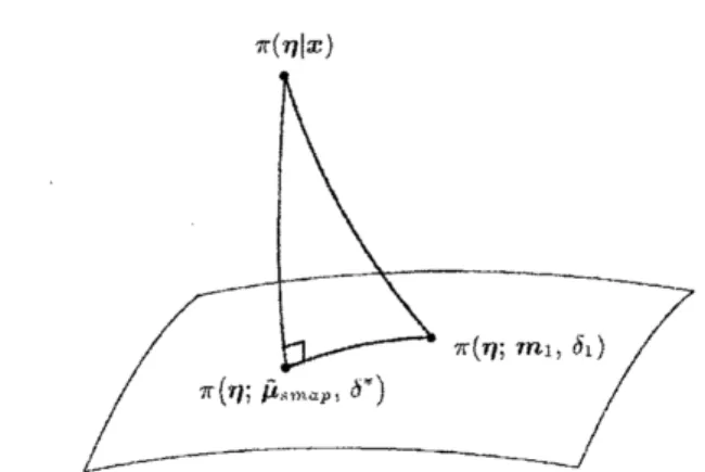
Thle following theorem gives a Pythagorean relationship holding $\mathrm{f}\dot{\mathrm{o}}1$ the conjugate prior

density. See Figure 1. Theleast inform atioti property isobtainedas

a

corollary.

Theorem 3.2.

Let $\pi(\eta)$ be $ar\iota y$ prior $der\iota s\mathrm{i}t?J\mathrm{i}\tau’$

.

$\mathrm{P}(x, m, \delta)defi^{1}ned$ by the condition (3.6), and write the

correspondingposterior density as $\pi(\eta|x)$. Then, the following $Pythago^{J}r.\epsilon’ a^{l}rl7^{\cdot}elatior\iota st\mathfrak{x}\mathrm{i}p$

$\mathrm{K}\mathrm{L}(\pi(\eta|x)_{\backslash }’\tau(\eta;m_{1}, \delta_{1}))=$ $\mathrm{I}\{\mathrm{L}$$(\pi(\eta|x), \tau)(\eta;\hat{\mu}_{sr;\iota a\mu}, \delta^{\mathrm{A}}))$

$+\mathrm{K}\mathrm{L}(\tau’(\eta;\hat{\mu}_{snlBp\rangle}\delta^{*}). \tau’(?l;\eta l_{1}, \delta_{1}))$ (3.7)

holds

for

any hyperparameters $m_{1}$ und$\delta_{1}$.

Proof.

Note that

KL$(\overline{l\mathrm{t}}(\eta|xx), \pi(\eta:m_{\mathit{1}}, \delta_{1}))-\mathrm{K}\mathrm{L}(\pi(\eta|x), \pi(\eta:\hat{\mu}_{s\tau nc\iota p_{j}}\delta^{*}\rangle)$

If

we

replace $\pi(\eta|x)$ with$’/\rceil^{-}(\eta;\hat{\mu}_{s’ r\mathrm{z}ap\}}\delta")$inthe right-handside,theexpected value be

comes

the Kullbaek-Leiblerseparatorfrom $\pi(\eta:\hat{\mu}_{sn\{\kappa\iota p}, \delta^{*})$ to $\pi(\eta:m_{1},\overline{\delta}1\rangle$

.

Thus, it is sufficient to

show that this replace nent does not change tlie above expected value. It followsthat

$\log\frac{\pi\acute{\{}\eta\hat{\mu}_{smap_{i}}\delta^{*})}{\pi(\eta im_{1},\overline{\delta}_{1})}=a_{1}^{T}\eta+a_{\mathit{2}}\mathrm{A}\tau_{f}^{\dot{f}}\acute,(\eta)+a_{\delta\backslash }\backslash$

where$a_{1}$, a2

an

ld $\mathrm{a}_{3}$

are

independent of$\eta$. They areexplicitly represented

as

$a_{1}=\delta^{*}h_{p+1}(\hat{\mu}_{s7nap}\}\hat{\theta}_{srnap}-\delta_{\mathrm{I}}h_{p\dashv- 1}(m_{1})\theta(m_{1})$,

$a_{2}=\delta_{1}h_{p+1}(m_{1})-\delta^{*}f\iota_{p+1}(\acute{\mu}_{srnp\iota p})$,

$a_{3}=+\delta_{1}h_{p+1}(m_{1})\{t’(\theta(m_{1}))-\delta^{*}l\iota_{p+1}(\mu_{\mathrm{s}\mathrm{r}\mathrm{n}\mathrm{a}\mathrm{p}})$ $\oint)(\hat{\theta}_{sn\iota a\rho})-K(m_{1}, \delta_{1})+K(\hat{\mu}_{s\prime\prime\iota ap}, \delta^{\star})$

.

Sincethe posteriordensity$\tau\downarrow(\eta|x)$ satisfies (3.6) by definition,therequired

$\mathrm{r}\mathrm{e}^{2}\mathrm{s}\iota 11\mathrm{t}$ is$\iota\tau \mathrm{b}\mathrm{t}\mathrm{a}\mathrm{i}\mathrm{l}\mathrm{z}\mathrm{e}\mathrm{d}$

.

$\square$

$\pi(\eta|x.)$

$7\ulcorner(\eta_{7}.$$\hat{\mu}$

$\backslash \uparrow’ \mathrm{x}ap-$ ,$\delta^{\mathrm{v}}\grave{)}$

$71^{\cdot}(\eta;$$m_{1}$,

$\delta_{1}\rangle/f$

$-\wedge$

$\ovalbox{\tt\small REJECT}$

Figure 1: TllePythagorean relationship holdingfor $\mathrm{t}1_{1}\mathrm{e}$ conjugate prior.

Now,we solve theminimization1problem ofthe followving$\mathrm{f}_{\mathrm{U}\mathrm{I}1\mathrm{C}}\mathrm{t}\mathrm{i}_{01}\mathrm{z}\mathrm{a}1$

$G[\pi(\eta)]=\mathrm{K}\mathrm{L}(\pi(\eta|x\rangle\backslash \tau’(\eta.\cdot x.1))$

.

Recall that the factor $b(\eta)$ $\mathrm{i}\mathrm{n}\mathrm{l}$ the prior density (3.1) is

$\mathrm{d}\mathrm{i}\mathrm{s}\epsilon$axded when deriving the stan-$\mathrm{d}\mathrm{a}\mathrm{r}^{*}\mathrm{d}\mathrm{i}\mathrm{r},\mathrm{e}\mathrm{d}$ posterior mode (3.2), Since we may look upon the

$\mathrm{s}$ ampling density $p(x^{\mathrm{z}}, \mu)=$ $\exp\{-d(x, \mu)\}a(x)$

as

the ptior density $\pi(\eta;x\grave, 1)$, the functional $G[\pi(\eta\rangle]$

can

be regarded

as

the information colltaitted in tl$\iota \mathrm{e}$ prior density $\pi(\eta)$

.

The following corollary gives the

minimizer of$G[\pi(\eta)]$

.

Corollary 3.3.

The conjugate priordensity(3.1) $n\iota \mathrm{i}n\mathrm{i}_{J\prime}^{l}\iota \mathrm{i}\wedge./es$ the$f\uparrow xr\iota ct\mathrm{i}onal$$G[\pi(\eta)]=KL(\pi(\eta|x\}_{\backslash }\pi(\eta;x, 1)$$)$

Proof.

Set $m_{1}=x$ and$\delta_{1}=1$ inTheorem 3.2. and$\mathrm{w}\cdot \mathrm{e}$ have

$G[\pi(\eta)]=G[_{J}\tau(\eta_{j}. m, \delta\}]+\mathrm{K}\mathrm{I}\lrcorner(\pi(\eta|x)_{\backslash }\pi(\eta j\hat{\mu}_{\mathrm{S}lnap\}}\delta^{*}))$.

This equality completes theproof. $\square$

Note that this corollary is closely related to discussions

on

the $1\mathrm{h}\mathrm{i}\mathrm{n}\mathrm{i}\mathrm{r}11r\mathrm{d}_{\vee}\mathrm{x}$ property of $\mathrm{t}$he

conjugate prior densityemployed by Morris (1983) and ConsonniandVeronese (1992). Weclosethissectionby$\mathrm{e}$mphasizing to

a

potentialrelationbetween thleconjugate

an

alysis

and the generalized linear model (GLM). Conjugatepriors for theGLM werestudiedby Chen and Ibrahim (2003). $\prime \mathrm{I}’1\iota \mathrm{e}\mathrm{G}\mathrm{L}\mathrm{M}$ is

bas ed 011 tlxe $\mathrm{s}\mathrm{a}\mathrm{I}\mathrm{I}1\mathrm{p}1\mathrm{i}_{1\mathrm{l}}\mathrm{g}$ density $p(.’\iota^{1}\mathrm{i}\mu)$ with lnean $\mu \mathrm{i}_{11}$

the one-para meter exponential $\mathrm{f}\mathrm{a}$ mily-$\mathrm{I}\iota$ is

known to $1_{1\mathrm{O}}1\mathrm{d}$ that $\log\{p(x;/\hat{x}_{\mathrm{k}\mathrm{J}\mathrm{L}})/\mathit{1}^{\mathrm{J}}(x:\mu)\}=$

$\mathrm{K}\mathrm{L}(p(y;;\hat{s}_{\mathrm{k}4\mathrm{L}})\dot, \mathrm{p}(\mathrm{y};\mu))$where$\hat{\mu}_{\mathrm{M}\mathrm{L}}=’.r$ is thernaximurn likelihoodestim ator. Thisis formally

rewritten as

KL$(\delta(y-\hat{\mu}_{\Lambda 1\mathrm{L}}), p(y;\mu))=\mathrm{K}\mathrm{L}(\delta(y-\hat{\mu}_{\mathrm{M}\mathrm{L}}), p(y;\hat{\mu}_{\mathrm{k}1\mathrm{J}_{\vee}}))+\mathrm{K}\mathrm{L}(p(y;\acute{\mu}_{\mathrm{M}\mathrm{L}}), p(y:\mu))$,

where$\delta(ry-A^{\cdot})$ is the$\mathrm{D}\mathrm{i}_{1}\cdot \mathrm{a}\mathrm{r},’ \mathrm{s}$deltafunction. A similarPythagorean relationship holds

approx-imately in tlleGLM. Com paaing withthe Pythagorean relationship (3.7) inTl

eorern

3.2.

we

learn tl at atypeof similarity lies betweentlte conjugate analysis and tlle GLM.

4. A Pythagoreanrelationship

Inthis and the followingsections$\mathrm{t}$he duaiPythagorean relationship$\mathrm{s}$arederived, each of

which manifests how the standardized posterior modedominates other $\mathrm{t}^{4}s\mathrm{t}\mathrm{i}\mathrm{r}\mathrm{n}\mathrm{a}\mathrm{t}\mathrm{o}\mathrm{r}\mathrm{s}$

.

The loss

functionsweadoptin the$\mathrm{t}\backslash \mathrm{v}\mathrm{o}$

cases

$\mathrm{a}1\mathrm{G}$ dualtoeachother. Assum ingthc

$\mathrm{t}\backslash \mathrm{v}\mathrm{o}$conjugate prior

densities, orthetwo types of $l$)($\eta\}$,

we

discusstl$1\epsilon^{1}$conjugate analysis separately.

First,

we

pursue anoptimalityoftire est$\mathrm{i}_{1}\mathrm{n}\mathrm{a}10\iota$ under the lossfunction$L(\hat{\mu}, \mu)=d(\hat{\mu}, \mu)/$

$h_{\mathrm{p}+1}(\hat{\mu})$, whenthereexists a non-negative function$b_{c}(\eta)$ such that

$\frac{\partial}{\partial m}$

.

$.\mathit{1}^{\cdot}\exp\{-\delta_{L}L(m\cdot, \mu)\}b_{\mathrm{c}}(\eta)d??=0$. $(4.1\rangle$

We set the integral in (4.1)

as

$\mathrm{e}\mathrm{x}\iota$)$\{-K(\overline{\delta}_{1})\}$. The density $\exp_{\mathrm{t}}^{J}-\delta_{1}L(m, \mu)+K(\delta_{1})\}b_{\iota}(\eta)$

belongs to the proper dispersion model introduced in Jorgensen $(1997, \mathrm{p}.\overline{\}})$. Setting $\delta_{1}=$

$\delta l\iota_{p+1}(m\rangle$, we

assu

me tltepriordensity

$r_{1_{\Gamma}}(\eta;m_{\dot{J}}\delta)=\exp\{-\delta d(m, \mu)+K(\delta l\prime_{p+3}(m))\}b_{\zeta}.(\eta)$. (4.2) It should bc noted that the

no

rmalizing constant depends on $m$ and 6 only through the

product$\dot{\delta}h_{p+1}(m)$

.

The conjugateprior density (4.2) hasthefollowingpropertywithrespecttothe expectation

ofthecxtended

can

onical para meter.

Proposition 4.1.

Underthe assumption (4.1) it holds

_for

any $m$ and $\delta>0$ that

where $\eta(m\rangle$ $=-(f_{1}(m)$,$\ldots$,$f_{p}(m\})^{T}$. Further, the posterior density

$C^{l}\mathrm{O}\mathit{1}’respo’\iota di\tau\iota g$ to $\pi_{\mathrm{t}}\cdot(\eta;m\dot, \delta)s$

atisfies

$\mathrm{E}[\eta-\hat{\eta}_{\mathrm{s}\prime nap}|\mathrm{T}l ,,(\eta:\hat{\mu}_{\mathrm{s}m\iota p}‘’\delta^{*})]=0$

.

Proof.

Differentiatingtheintegral in (4.1) withrespect to $\theta(m)$,

we

have

$\int.\{\eta(m)-\eta\}\exp\{-\delta_{1}L(m, \mu\}\}b_{c}(\eta\prime 1d\eta=0$ (4.3)

for any$m$ and $\delta_{1}>0$

.

Setting $\delta_{1}=\delta f\iota_{p+1}(m)$, we $01_{\mathrm{J}}\mathrm{t}\mathrm{a}\mathrm{i}\mathrm{n}$ tlle $\mathrm{f}\mathrm{o}$

rmer

part.

Th

cozcrn

3.1 yields that the corresponding posterior density $\mathrm{i}_{\mathrm{b}}$ expressed $\mathrm{a}5\prime \mathrm{T}_{C}(\eta;\hat{\mu}_{sr’ \mathrm{z}\alpha\rho}$,

$\delta’)$. Notingthat $\hat{\eta}_{sr\iota ap},=\eta(\hat{\mu}_{s\tau\tau\iota ap}|\rangle$,

we see

that the latter part follows obtain thle

$\mathrm{f}\mathrm{o}$

rmer

part. $\square$

Thisproposition is an extension of Proposition 4.5 $(\mathrm{i}\mathrm{i},)$ in Yanagimoto and Ohnishi (2005a),

wherethe sampiingdensityis restiictedto$\mathrm{b}\mathrm{c}^{\mathrm{I}}$inthe$\mathrm{n}\mathrm{a}\mathrm{t}\mathrm{u}\mathrm{I}^{\cdot}\mathrm{a}\mathrm{l}$ exponential family. Thisextension

is realisedby introducing$\eta$ suitably.

$\backslash \mathrm{h}\tilde{\prime}\mathrm{e}$ clarify im plicationsof Propositionil through the following example wherethe

sarn-pling density is inthe natural exponentialfamily (1.1).

Example

_4.1.

Set $fj(\mu,$} and $f\iota_{\mathcal{J}}(x)(\iota. =1_{\mathrm{j}}2)$ in $\mathrm{t}11\langle^{1}$ natural exponential family (1.1) as in

the form

cr

part of Exa mple2.1. Suppose that the

assum

ption(4.1) is satisfied, that is, the

no$\mathrm{r}1\mathrm{n}\mathrm{a}1\mathrm{i}\mathrm{z}\mathrm{i}_{1\mathrm{l}}\mathrm{g}$constant $\mathrm{i}1\mathrm{J}(4.2\rangle$ depends only on

$\overline{\delta}$. Then, the posterior mean of$?/=\phi’(\mu\grave{)}$ is $\phi’(\hat{\mu}_{b\mathrm{V}lb\mathcal{U}\beta})$ with$\hat{\mu}_{srr\iota\iota p},‘=(.c +\mathrm{f}\overline{)}\prime\prime l)/(1+\delta)$

.

Next, $\backslash \mathrm{v}\mathrm{e}$ deal with

$\mathrm{t}\mathrm{l}\iota \mathrm{e}$

case

where the sampling density is defined on

$\mathbb{R}^{+}$ and set

$f.j$$(\mu,$ and $h_{j}(x)(\mathrm{i}=1_{\dot{l}}2$

}

as

inthe l.a$\mathrm{t}\mathrm{t}\epsilon^{1}1$’ part ofExample 2.1. The

assum

ption (4.1) is equivaleut

to tlleonethat the

no

rmalizingconstant in (4.2) isafunction of $\delta_{7\prime}\iota$

.

Under thisassumptionl

the posterior $\mathrm{m}$

ean

$\mathrm{n}\mathrm{f}$_{$\psi(7//\backslash =\psi’(\phi’(\mu)\rangle$} is $\psi(\acute{\varphi}(\hat{\mu}_{6t\prime\iota ap}$

}

$)$

.

Now, let us derive

a

Pythagorean xelatiollshiI)withrespect toposterior risks. Proposition 4.2.

Under the assumption (4.1) the Pythagorean relationsf$\iota \mathrm{i}\chi_{J}$

$\mathrm{E}[L(\hat{\mu}, \mu\rangle-L(\hat{\mu}_{\mathrm{S}\dagger\iota ap},, \mu)-L(\hat{\mu},\hat{\mu}_{b\mathcal{T}\prime\iota c\iota p})|\pi_{c}(\eta;\hat{\mu}_{6\mathit{7}\mathfrak{l}l(\iota p}(’ \delta^{*})]=0$ (4.4)

holds

for

any estimator $\hat{\mu}$. $Th^{r}us_{f}thc$ $sta$}

$\iota da^{C}rdizc^{\mathrm{J}}d$posterior$r\prime lode$ _Psrn

$\iota a\rho$ is

$opt\mathrm{i}r\tau\iota u7’\iota$un$dc^{\mathrm{J}}r$

the loss $L(\hat{\mu}.\mu)$

.

Proof.

It follows$\mathrm{f}\mathrm{i}^{\backslash }\mathrm{o}\mathrm{r}\mathrm{r}\iota$ the identity (2.9) that

$L(\hat{\mu}, \mu)-L(\hat{\mu}_{B7nup}, \mu)-L(\hat{\mu},\acute{\mu}_{sr\prime\not\supset ap})=\{\theta(\hat{\mu})-\theta_{67\prime\lambda\prime\iota p}^{\mathrm{A}}\}^{T}(\hat{\eta}_{sn\iota\zeta\iota p}-\eta\rangle$

.

$(4‘ 5)$

Note that $\theta(\mu$

}

$-\hat{\theta}_{br’\iota ap}$ is constant$\mathrm{n}\mathrm{t}$ in

17. Thus, the latter part of Proposition 4.1 yields the

Pythagoreanrelationship(4.4). The$\mathrm{o}\mathrm{p}\mathrm{t}\mathrm{i}_{1\mathrm{U}\mathrm{U}1\mathrm{K}1}\mathrm{p}\iota^{\backslash }\mathrm{o}\mathrm{p}\mathrm{e}\mathrm{r}\mathrm{t}\mathrm{y}$of$\hat{\mu}_{sm\alpha p}$follows

$\not\in_{\mathrm{L}}\mathrm{o}\mathrm{m}$$\mathrm{t}1_{1}\mathrm{i}\mathrm{s}$$\mathrm{P}\mathrm{y}\mathrm{t}\mathrm{l}\iota \mathrm{a}\mathrm{g}\mathrm{o}\mathrm{r}\mathrm{e}\mathrm{a}\mathrm{I}\mathrm{l}$

$\square$

We derive an extended version of the Pythagoreanrelationship in Proposition 4.2. This is done by modifyingthe loss function$L(\hat{\mu}, \mu)$ for anappropriate choiceof$b(lJ\rangle$ intheprior

density (3.1). Suppose that there exista positive function$I(m)$ alld

a

non-negatrvefunction

$\overline{b}_{c}(\eta)$ such that

$\frac{\partial}{\partial m}/\cdot\exp\{-\delta_{1}\mathrm{I}(m)L(m_{/}.\mu)\}\tilde{b}_{c}(\eta)d\eta=0_{\backslash }$. $(4.6^{\cdot}1’$ and wc writethleintegral in (4.6)

as

$\exp\{-\tilde{K}(\delta_{1})\}$

.

$\mathrm{T}\mathrm{h}\zeta^{1}$assumption(4.6) is weaker than(4.1),

since the forlllCl. allows $I(m)$.

The priordensity

we assume

on$\eta$ isoftheform

$\overline{\pi}_{c}(\eta:m, \delta)=\exp\{-\delta d(m, \mu)+\overline{\mathrm{A}^{r}.}\{\frac{\delta h_{p+1}(m)}{I(m)})\}\tilde{b}_{\mathrm{c}}(\eta)$.

Theorem3.1 meansthat the correspondingposterior density is expressed

as

$\tilde{\pi}_{c}(\eta;\hat{\mu}_{sn\iota\iota\iota p},$ $\delta^{*}\}$

.

A modified Pythagorean $\mathrm{r}\mathrm{e}1\mathrm{a}\mathrm{t}\mathrm{i}_{01}1\mathrm{s}\mathrm{h}\mathrm{i}\mathrm{p}$is derived under the loss 1$(\hat{\mu})L(\hat{\mu}_{\gamma}\mu)$. It should be

noted that the posterior risk diffelcllce is expressed through the Kullback-Leiblerseparator

between the two ($\mathrm{p}\mathrm{r}\mathrm{i}\mathrm{o}\mathrm{r}\uparrow$densities.

Proposition 4.3.

Underthe

assu

mption (4.6) set $\pi\tau(\eta;m, \delta_{1})$ $=\mathrm{e}\mathrm{x}1)\{-\overline{\delta}1l(rn)L(m, \mu)+\tilde{R}^{\nearrow}(\delta_{1})\}\tilde{b}_{c}(\eta)$ . The foilowing

_modified

Pythagorean $L^{-}el(ztlonship$

$\mathrm{E}[I(\hat{\mu})L(\hat{\mu}_{\backslash }\mu)-I(\hat{\mu}_{sr\prime\iota ap})L(\hat{\mu}_{67nap}, \mu\rangle|\overline{\pi}_{\mathrm{c}}(\eta_{j}\hat{\mu}_{srn\iota\iota p}, \mathit{5}^{*}\rangle]$

$= \frac{1}{\delta_{1}^{*}}\mathrm{K}\mathrm{L}$$(\pi_{I}(\eta;\hat{\mu}_{s\tau\prime\iota \mathrm{f}lp}, \delta_{\rceil}^{*})\dot,$ $\pi_{\Gamma}(\eta \mathrm{i}\hat{\mu}, \delta_{\mathrm{t}}^{*}))$ (4.7)

holds

for

any estianator$\hat{\mu}$ there $\delta_{1}^{*}=\{f\iota_{2\}+1}(x)+\delta f\prime_{\beta+1},(m)\}/I(\grave{\mu}_{s^{\mathit{1}}’ nup})$. Consequently, the standardizedposteriormode $\hat{\mu}_{\mathrm{s}r’\iota ap}$ is optimum under

$tf\iota e$ loss $I(\hat{\mu})L(\hat{\mu}, \mu)$.

Proof

Acalculation ofth$1\mathrm{C}$right-hand side of (4.7) gives

$\frac{1}{\delta_{1}^{*}}\mathrm{K}\mathrm{L}(\pi_{I^{(_{\backslash }\eta;\tilde{\mu}_{\Delta taap},\delta_{1}^{\star})}}, \pi\gamma(\eta;\acute{\mu}_{\tau}.\tilde{\delta}_{1}^{*}))$

$=\mathrm{E}[I(\hat{\mu})L(\hat{\mu}_{\dot{r}}\mu)-I(\hat{\mu}_{\mathrm{s}rnap}\}L(\hat{\mu}_{b\prime\uparrow\iota\iota p}‘’\mu)|\tau_{1/}(\eta;\mu_{srnap}^{\mathrm{A}}, \delta_{1}^{*})]$

The equality (2.10) and the expression (3.4) of $\delta^{*}$, together with tlte expression of $\delta_{1}^{*}$ in

Proposition 5.1, give

$\delta_{\mathrm{L}}^{*}I(\mathrm{A}\mu_{sm\mathrm{r}\iota p})L(\hat{\mu}_{srt\iota ap}, \mu\grave{)}=\delta^{*}d(\hat{\mu}_{b7nav}..\mu)_{!}$.

$\tilde{K}(\delta_{1}^{*})=\tilde{K}(\frac{\delta^{*}h_{p\}1}(\grave{\mu}_{sr\prime\iota ap})}{I(\hat{\mu}_{s;pap})},)$

.

Thus, we

see

that the posterior density$\tilde{\pi}_{c}(\eta;\hat{\mu}_{brr\iota\alpha p}, \delta^{*})$ is equal to $\pi_{l}(\eta;\hat{\mu}_{s\iota a\mathrm{p}}"’$$\delta_{1}^{*},$}, which

completes the proof. $\square$

Another expression of the term $L(\hat{\mu},\hat{\mu}_{\mathrm{S}lr\iota ap})$ in Proposition 4.2 is obtained

as

$L( \hat{\mu}_{2}\hat{\mu}_{sntap})=\frac{1}{\delta_{1}^{*}}\mathrm{K}\mathrm{L}(\pi_{1}(\eta;\grave{\mu}_{b7\prime\iota ap}’, \delta_{1}^{*}),$ $\pi_{1}(\eta;\hat{\mu},\tilde{\delta}_{1}^{\star_{\mathrm{r}}}))$

where $\pi 1$$(\eta;m,, \delta_{1})$ $=\exp\{-\delta_{1}L(m, \mu)+K(\delta \mathrm{l}\}\}b_{(},(\eta)$ and$\overline{\delta}_{1}^{*}=/\iota_{p-\vdash 1}(x)$ $+\delta h_{p\dagger\lfloor}$_$(5.1)$

.

Thehyperbola density (2.12) provides

us

with

an

illustrative

exam

ple of Proposition 4.3, where

a

modified loss $\mathrm{f}\mathrm{u}11_{J}‘ \mathrm{t}\mathrm{i}\mathrm{o}11$$I(\hat{\mu})L(\ell\iota. \mu)\mathrm{A}$ is

more

familiarthanthe original

one

$L(\hat{\mu},\dot, \mu)$.

Example

_4.

$\kappa^{\beta}i$

.

The dual

convex

functionsare$\psi(\eta)=c\mathrm{o}\mathrm{s}\mathrm{h}(\sinh^{-1}\eta)\mathrm{a}I1(1\dot{q}’(\theta)=\theta\sinh(\mathrm{t}\mathrm{a}11\mathrm{h}^{-1}\theta)-$ $\mathrm{c}\mathrm{o}‘ \mathrm{s}\mathrm{h}(\mathrm{t}\mathrm{a}\mathrm{r}1\mathrm{h}^{-1}\theta)$ inthle hyperboladensity$p_{\mathrm{H}}(\prime x;\mu\backslash , \tau)$ in (2.12). Thus, the lossfunction $L(\hat{\mu}, \mu)$

is of the form $L(\hat{\mu}$

}

$\mu\rangle$ $=\{\mathrm{c}\mathrm{o}\mathrm{s}11(\hat{\mu}-l^{l})-1\}/$ case$\hat{\mu}$. A $\mathrm{f}\mathrm{a}$miliarloss function in the literature is $I(\hat{\mu})L(\grave{\mu}, \mu)=$ {$j\mathrm{o}\mathrm{s}1\mathrm{x}(\hat{\mu}\cdot-\mu)-$ $1$, which is obtain ed by setting $I(\mu$

}

$=(^{\backslash }\mathrm{o}\mathrm{s}\mathrm{h}\mu$. If

we

choose

$b(\eta)$ as $\tilde{b}_{c}(\eta)=d\mu/d\eta=1/\cosh(\mathrm{s}\mathrm{i}\mathrm{r}1\mathrm{h}^{-1}\eta)$

,

then the integral

$J_{-\mathrm{m}}^{\propto)}.\exp\{-\delta_{1}I(ln)L(Ir\iota, \mu)\}\tilde{b}_{\mathrm{L}}(\eta)d\eta=J_{-\infty}^{\infty}.\exp\{-\delta_{\mathrm{I}}\cosh(m-\mu)\}d\mu$

isinldepeIxdellt of$/n$. NotethattheKuliback-Leiblerseparator from$p_{\mathrm{H}}(\mu;m_{1}.\delta)$to$p_{11}(\mu\}. \prime\prime\iota_{J}.., \delta)$

is calculatedas

$\mathrm{K}\mathrm{L}((rr\iota_{1}, \delta)$, $(_{7n\underline{\prime y}}, \delta^{-}))=\frac{I_{1^{\nearrow}1}(\delta)}{\mathit{1}\mathrm{i}_{0}’(\delta)}\{\cosh(\uparrow n_{1}-?\tau\iota_{2})-1\}$

.

For

an

arbitrary estimator $\hat{\mu}$Proposition 4.3 gives the following modifiedPythagorean

iela-tionship

$\mathrm{E}[\cosh(\hat{\mu}-\mu)-\cosh(\hat{\mu}_{st;\iota e\epsilon p}-\mu)|p_{\mathrm{H}}(\mu_{\}.\hat{l^{l}}smap’\delta_{1}^{*})]=\frac{1}{\delta_{1}^{*^{\vee}}}\mathrm{K}\mathrm{L}((\hat{\mu}_{s\tau\prime*\iota p}‘’\delta_{1}^{*})\dot{\prime}(\hat{\mu}_{\backslash }\grave{\delta}_{1}^{*}))_{7}$

where tauh$\mu\wedge ymap=\{\tau \mathrm{s}\mathrm{i}_{11}\mathrm{t}_{1’1j}.+\delta \mathrm{s}\mathrm{i}_{\mathrm{I}1}\mathrm{h}_{7\prime}\iota\}/$

{

$\tau$rosh$x+\delta$case$r;\iota$

}

and$\delta_{1}^{*}=\{\tau^{\mathit{2}}.+\delta^{2}+2\tau\delta\cosh(.’\iota-$

$7ll,)\}^{1/2}$.

5. A dual version of the Pythagorean relationship

We

move

to the

case

of an alternative loss function $L(\mu_{7}\hat{\mu}$

},

dual to $L(\hat{\mu}, \mu)$

.

Another

$\mathrm{c}\mathrm{o}\mathrm{r}1\mathrm{j}_{11}\mathrm{g}\mathrm{a}\mathrm{t}\mathrm{e}$prior densitywhich is ina

sense

dual to $\pi_{c}(\eta jm, \delta)$ in (4.2) is dealt with. Setting

$b(\eta)=1$, we$\mathrm{a}\mathrm{s}\mathrm{s}\iota \mathrm{u}\mathrm{l}\mathrm{l}\mathrm{e}$ thepriot density

$\pi_{7l},\acute{(}\eta;m$, $\delta)$ cx$\exp\{-\delta d(m_{7}\mu)_{f}^{1}$ (5.1)

with respect to $\mathrm{t}1_{1}\mathrm{e}$ Lebesgue

measure

on

$\eta$. Wlten the sax1lpliug density is in the regular

natural exponential $\mathrm{f}\mathrm{a}$mily, thisprior density reduces to what iscalled thleDY prior density.

We atte npt here to extend Theorem 2 in Diaconis and $\mathrm{Y}1\mathrm{v}\mathrm{i}\mathrm{s}\mathrm{a}1_{\acute{\mathrm{t}}}\mathrm{e}1$(1979) in various ways,

For this

purpose we

$\mathrm{a}\mathrm{s}\mathrm{s}$

ume

tllat $\lim_{\eta_{j}arrow\overline{\eta}_{J}}d(m,$

$\mu.$

}

$=\infty$ and

$\lim_{\eta j^{arrow\underline{\eta}_{\dot{\lrcorner}}}}d(m, \mu)=\infty$ for

$\mathrm{j}=1\mathrm{L}’\cdots$ ,p. $(5.2\rangle$

In the above$\overline{\eta}_{j}=\overline{\eta}_{j}(\eta(j\rangle)$and$\underline{\eta}_{j}=\underline{\eta}_{j}(\eta(j))$

are

respectively theupperandthe lower boundary

point when$\eta(j)=(\eta_{1}, \ldots, \eta j-3,Y/j+1, \ldots., r/_{\mathrm{P}})^{T}$ are fixed. Rougllyspeaking, th is

ass

umption irrrplics thatthe density vanishes at theboundary. The following$\mathrm{P}^{\mathrm{I}\mathrm{Q}}\mathrm{p}oi_{3}\mathrm{i}\mathrm{t}\mathrm{i}\mathrm{o}\mathrm{x}1$ claimsthat tlte

priordensity (5.1) has aproperty dual to theone in Proposition4.1.

Proposition 5.1.

Underthe assumption (5.2) it holds

_for

any $m$ and $\delta>0$ that

Itiaddition, the posterior density corresponding to$\pi_{r’\iota}(\eta jm, \delta)$ satisfies

$\mathrm{E}[\theta-\hat{\theta}_{\mathrm{b}r\prime\iota ap}|\pi_{r\iota},(\eta_{\backslash }.\hat{\mu}_{s\mathrm{r}nap}, \delta^{\wedge})]=0$.

Proof.

It followsfrom (5.2) that

$\mathit{1}_{\underline{\eta}_{j}}^{\overline{l}_{\mathrm{j}}}.\frac{\partial^{\Gamma}}{\partial\eta_{j}}\exp\{-\delta d(m, \mu|\}\}d\eta_{j}=0$

for $j’=L$$\ldots$,$p$. We have from (2.6) and $(\mathrm{A}.4\grave{)}$

$\frac{(;t}{\partial\eta_{j\prime}}d(m, \mu,)=-l_{j}\}(m)+’\frac{h_{j}(\mu)}{f\iota_{p+1}(\mu)}h_{p+1}(m\grave{)}=l\iota_{p+1}(m)\{\theta_{j}-\theta_{j}(m)\}$

.

Com binin${ }$ these,

we

obtain the

$\mathrm{f}\mathrm{o}$

rmer

part.

The proofofthe latter part isparallel to that ofthe latter part of$\mathrm{P}_{1}\mathrm{o}\mathrm{p}\mathrm{o}\mathrm{s}\mathrm{i}\mathrm{t}\mathrm{i}\mathrm{o}\mathrm{n}4.1$. $\square$

Now, let

us

deriveaPythagorean relationshipwithrespect tothe$1\mathrm{c}_{\mathit{1}}\mathrm{s}\mathrm{s}\mathrm{f}_{\mathfrak{U}\mathrm{n}(j}\mathrm{t}\mathrm{i}_{011}L(\mu,\hat{\mu})=$

$d(\mu,\hat{\mu})/h_{p+1}(\mu.)$

.

Note that the loss functionand tlicproperty of thle prior density

are

dual

to those inthe previous Pythagorean relationship (4.4). Proposition 5.2.

Underthe assumption $(\overline{:\supset}.2)$ the Pythagorean relationship

$\mathrm{E}[L(\mu,\grave{\mu})-L(\mu_{\backslash }\hat{\mu}_{st\prime\iota c\iota p})-L(\hat{\mu}_{smap}\dot,\grave{\mu}\}|\pi_{rn}(\eta:\hat{\mu}_{\mathrm{b}7\prime\iota a\nu}, \delta^{\mathrm{f}})]=0$ (5.3)

holds

_for

any estimator $\hat{\mu}$. Therefor\^e the $standu’.d\mathrm{i}zed$ posterior $?r\iota ode$ $\hat{\mu}_{6?’\iota ap}$ is optimum

under$\cdot$the loss _{$L(\mu.\acute{\mu}\}$}

.

Proof.

The proof is parallel tothat of Proposition 4.2. Instead of the identity (4.5), we use

$L(\mu,\hat{\mu})-L(\mu_{2}\hat{\mu}_{b\mathrm{f}rlap})-L(\hat{\mu}_{\mathrm{S}\tau t\iota ap},\hat{\mu},)=(\theta-\hat{\theta}_{sm(\prime p})^{T}(\hat{\eta}_{smup}-\hat{\eta})_{\backslash }$

where $\hat{\eta}$ is theestimator equivalent to $\hat{\mu}$.

$\square$

Next, a modification ofthe Pythagoreanrelationship (5.3) is dealt with. $\mathrm{W}^{\Gamma}\mathrm{e}$ adopt

a

loss

function$J(\eta)L(\mu,\grave{\mu}$

}

with $J(\eta)$ beinga positive function. $\ulcorner I\mathrm{h}\epsilon^{\iota}$ priorden sitywe

assume

isof

the fonn

$\tilde{\pi}_{rn}(\eta;m, \delta)\mathrm{r}\mathrm{x}\exp$

{-fftl

$(m,$ $\mu)$

}

$/J(\eta)$. (5.4) It follows from Theorem3.1 that the above priordensity is alsoconjugate, axldalso that th$1\mathrm{G}$

posterior density is given

as

$\tilde{\pi}_{t’ t}(\eta:\hat{\mu}_{6map},$ $\delta^{*}\rangle$. Here again

we

assume

theregularity condition

(5.2), We learn that amodifiedPythagorean relationship holds under the loss $J(\eta)L(\mu_{?}\hat{\mu})$

.

Note that tlle third term in tl$\mathrm{z}\mathrm{e}$ posterior expectation in the following proposition is not

Proposition 5.3.

Under the

assum

ption $(\check{\mathrm{D}}.2)$ the

modified

Pythagorean relationship

$\mathrm{E}[J(\eta)L(\mu,\hat{\mu})-J(\eta)L(\mu,\hat{\mu}_{smu\rho})-.I(\eta)L(\hat{\mu}_{9\prime nal^{27}}\hat{\mu})|\overline{\pi}_{r\prime l}(\eta;\hat{\mu}_{s\prime\prime\iota a\rho}, \delta^{\Lambda})]=0$ $($5.$\overline{\mathrm{e}‘ \mathrm{J}})$

holds

_for

any estimator $\mu^{\nearrow}$. Thus, the stand$a\gamma.d\dot{\tau.}zed$posterior $\tau r\iota ode\hat{\mu}_{srn\iota\iota p}$ is optimum under

the loss $J(\eta)L(\mu,\hat{\mu}\rangle$.

Proof.

Co mparing the two prior densities(5.1) and(5.4),we seethat$J(\eta)\tilde{\pi}_{\rho’\}}(\eta;\hat{\mu}_{smap}, \delta^{*})$sc

$\overline{\}}m(\eta;\hat{\mu}_{smap\backslash }\delta^{*})$

as

functionsof$\eta$

.

Tiie modified Pythagorean$l1$relationship (5.5) is a

rewrit-tenversionof the original

one

(5.3). $\square$

Interestingly, the$8\mathrm{t}\mathrm{a}\mathrm{l}\downarrow \mathrm{t}\mathrm{l}\mathrm{a}\mathrm{I}^{\cdot}\mathrm{d}\mathrm{i}\mathrm{z}\mathrm{e}\mathrm{d}$ posterior modeisopti mumforallthle loss functionsin

Propo-sitions 4.2, 4.3, 5.2 and 5.3.

Let $\xi=(\xi_{1\backslash }\vee\cdot$.

’$\xi_{\mathrm{P}J}^{1^{T}}$ be a new paral eter vector $\iota\backslash$hich has

a

$011\mathrm{P},- \mathrm{t}\mathrm{o}-\prime l11\mathrm{C}$ corresponden

ce

with$\eta$. We write the Jacobianof

$\mathrm{t}_{1}\mathrm{f}1\mathrm{e}$parametertransformation as $\partial\xi/\acute{\iota}J\eta$. Consider $\mathrm{t}1_{1}\mathrm{e}$ prior

density cxp$\{-\delta d(m, \mu)\}$ with respect to the Lebesgue 1ncasrue ou $\xi$. Especially when tlie

sampling density is in thle exponentialfamily, this priordensity is called standard conjugate

by Consonni and Veronese (1992). The prior density is equivalent to (5.4) with $1/J(\eta)=$ $|\partial\xi/\cdot\partial\eta|$

.

Thlefollowingexam plegives implications ofPropositions 5.2 aJld$\iota \mathrm{J}\cdot 3\ulcorner$tothenatural

cxpo-nential family (1.1).

Example 5.$f$

.

Let us

assume

that thena rural exponential$\mathrm{f}\mathrm{a}\iota \mathrm{m}\mathrm{i}\mathrm{l}\mathrm{y}$ $(1.1)$ isregular, $\mathrm{i}.\mathrm{e}.\uparrow$ that its

canonica 1space is

assu

med to beopen. This

assu

mption im plies that

$\etaarrow 1\mathrm{i}_{\mathrm{l}_{\frac{\mathrm{n}}{;\}}}}\mathrm{K}\mathrm{L}(?n, \mu)=\infty)$ and $rl_{-}\prec\prime\prime 1\mathrm{i}\mathrm{r}\mathrm{I}1\mathrm{K}\mathrm{L}(\prime\prime\iota, \mu)=\infty$,

where $\mathrm{K}\mathrm{L}(\mu_{1}., \mu_{2})$ is the Kullback-Leibler separator from $p(x; \mu\rfloor)$ to $p(\alpha,;\mu_{arrow\prime}‘)$. Thus, the

assumption (5.2) is satisfied. It is known that the DY prior density exists for

a

regular

natural exponentialfamily. It isofthe fonn

$\pi_{\mathrm{r}t\iota}(\eta;m, \delta)=\tau\downarrow \mathrm{r})[searrow]’(\eta\cdot, \tau;\overline{\iota}, \delta)\alpha \mathrm{e}\wedge \mathrm{x}\mathrm{p}$

{

$-\delta \mathrm{K}\mathrm{L}$(to, $\mu,)$

}

with respectto the Lebesgue measure

on

$7f$

.

Then,thestandardized posterior mode $\hat{\mu}_{srn\alpha p}=$

$(x +\delta m)/(1+\delta)$ isopt _imum withrespect to the loss $\mathrm{K}\mathrm{L}(\mu,\hat{\mu})$.

Next,

we

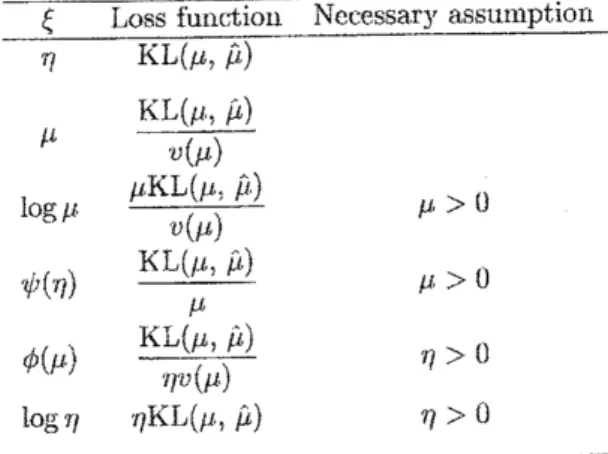
introduce a new parameter$\langle$ $=\xi(\eta)=\xi(\phi’(\mu))$, and consider the priordensity $\tilde{\pi}_{m}(\tau^{\backslash }/:7\Gamma l,, \delta)$$\alpha$$\exp\{-\delta \mathrm{K}\mathrm{L}(?r\iota, \mu)\}|\frac{d\xi}{\{fr\prime}.|$

.

The function $\xi(\eta)$ is assumed to be strictly increasing. Several cases of$\xi(7’)$ and the

corxe-spondiugIoss function$J(’/)L(\mu,\hat{\mu})$

are

given inTable 1, where titefunction $v(\mu)$ denotes the

Table 1: Examples of the parameter

4

and the loss function $J(\eta)L(\mu,\hat{\mu})$ in tlle natural

exponential family

$\frac{\overline{\xi \mathrm{L}\mathrm{o}\mathrm{s}\mathrm{s}\mathrm{f}}\mathrm{u}\overline{\mathrm{I}1\mathrm{C}\mathrm{t}\mathrm{i}\mathrm{o}\mathrm{n}\mathrm{N}\mathrm{e}\iota \mathrm{e}\mathrm{s}\mathrm{s}\mathrm{a}x_{3’}\mathrm{a}\mathrm{s}\mathrm{s}\iota\iota 1\mathrm{n}\mathrm{p}\mathrm{t}\mathrm{i}\mathrm{o}}11-}{\eta \mathrm{K}\mathrm{L}(\mu,\hat{\mu})}.$

.

$\mu$ $\frac{\mathrm{K}\mathrm{L}(\mu_{\}\acute{\mu})}{v(\mu)}$

$\log\mu$ $\frac{\mu \mathrm{K}\mathrm{L}(\mu_{\dot{J}}\hat{\mu})}{v(\mu)}$ $\mu_{J}>0$

$\psi(\eta)$ $\frac{\mathrm{K}\mathrm{L}(/x,\hat{\mu})}{\mu}$ $\mu>\mathrm{U}$

$\phi(\mu)$ $\frac{\mathrm{K}\mathrm{L}(\mu_{\}}\grave{\mu})}{\eta v(\mu)}$ $\eta>\mathrm{t}]$

$1_{0_{\acute{P}3}^{\mathrm{J}}\mathit{7}\int}$ $\eta \mathrm{K}\mathrm{L}(\mu,\hat{\mu})$ $\eta\backslash /0$

6.

Examination

ofthe non-singularity condition

The aimofthissection istomake regularity conditions weaker. Our$\mathrm{d}\mathrm{i}\mathrm{s}\mathrm{c}.\mathrm{u}\mathrm{s}\mathrm{s}^{\neg}\mathrm{i}\mathrm{o}11\mathrm{s}$inSections 2 through 5

were

based on thle non-singularity condition (C.4). However, the conjugate

analysis is possible without this regularity condition to bollle extent. An example is thevon

Mises distribution, the conjugate analysis of which

was

studied by Mardia and El-Ato rn (1976).

Let $F_{p,p+1}(t)$ denote the $p\mathrm{x}$ $(p+1)$ matrixwhose $(\mathrm{i},j)\mathrm{t}1_{1}$component is $.$

$\partial Jj(t)/\partial ti(1\leq$

$\mathrm{i}\leq p$, $1\leq j\leq p+1)$

.

In place of(C.4) requiring the non-singularity of $F_{p,p}(t)$ alld

$(\mathrm{C}.5^{\mathrm{t}})_{7}$

we

here

assum

$\mathrm{e}$ tllefollowingregularity condition

(C.4’) rank$F_{p,p+1}(t)$ $=l)$foi any $t$.

In order to make tlic difference betw

een

(C.4) and $(\mathrm{C}.4’.)$ clear, we consider the $\mathrm{v}\mathrm{o}\iota\iota$ Mises case. Whether we set $f_{1}(t)=-\cos t$, or $f_{1}(t)=$ -$\mathrm{s}\mathrm{i}_{11}\mathrm{t}$, the condition (C.4) is xiot satisfied.

However, thc rank of the 1 $\mathrm{x}_{\sim^{1}}$

.

matrix $(\mathrm{s}\mathrm{i}\mathrm{u}t, -\cos t)$ is equalto

one

for any$t$, that is, (C.4’)

issatisfied.

Since itseem$1\mathrm{S}$ difficultto definetlle extendedcanonical

param

eter, we assum

$\downarrow \mathrm{e}$prior

den-sities

on

the parameter $\mu$. The

assu

uted prior density has the form

$\pi(\mu;m., \delta)\alpha$$\exp\{-\delta d(m_{\dot{i}}\mu)\}c(\mu)$, $(6.1\rangle$ where $c^{l}(\mu)$ is anappropriate non-negativefunction.

Proposition 6.1.

Suppose that the standardized posterior mode (3.2) is uniquely determined. Then, the prior

density (6.1) isconjugate.

Proof

The proofis si milar to that ofTheore$\ln 3.1$. We prove that th_le right-hand side

of (3.5) is proportional to $d(\hat{\mu}_{smc\iota p}, \mu)$

.

It suffices to $\mathrm{S}$}$\mathrm{I}\mathrm{O}\mathrm{Y}\mathrm{V}$ that the two vectors $\hat{h}(x)+$

$\delta\tilde{h}(m)$ an$1\mathrm{d}h\sim(\hat{\mu}_{smup})$

are

proportional where $\tilde{h}(t\rangle$ denote the $(p+1)$-dimensional vector

$(.\partial/\partial\mu)\{d(x., \mu)+\delta\iota l(m, \mu)\}|_{\mu=\hat{\mu}_{\aleph\eta?a\mathrm{u}}}=0$. This is expressed in a matrix representation

as

$F_{p.p+[perp]}(\hat{\mu}_{sr’\iota ap})\{\tilde{h}(x)+\delta\tilde{h}(m)\}=0$

.

The equality (2.3) with $a=\hat{\mu}_{sn\iota\iota\iota p}$ is rewritten as

$F_{p.p+1}(\hat{\mu}_{smap})\tilde{h}(\hat{\mu}_{s\iota ap}")=0$

.

Note tlat the lIlatrix $F_{p,p-\vdash 1}(\mu_{srnap})$ 1s offull $1^{\cdot}\mathrm{a}\mathrm{l}\mathrm{l}\mathrm{k}$. It follows

from the theoryof linear algebra that thereexists $\overline{\delta}^{*}$ sudr that

$\tilde{h}(x)+\delta\overline{h}(m)=\delta^{*}\tilde{h}(\hat{\mu}_{\mathrm{S}\mathit{7}’ bap})$. (6.2)

Thus, thedesired proportionality

$d(x, \mu)+\delta d(m, \mu)-d(x,\hat{\mu}_{srnl\lambda p})-\vec{\delta}d(m_{j}\hat{\mu}_{6map})=\delta^{i}d(\hat{\mu}_{sn\iota\alpha p}, \mu)$

is obtained, _Tlle existence assumptionof$\hat{\mu}$smap guarantees that $\delta^{*}>0$

.

Thus, we

see

that

the posterior density is expressed

as

$\tau_{\mathrm{t}}(\mu_{\mathrm{t}}.\hat{\mu}_{bmap}, \delta^{*})$

.

$\square$

Discussions similarto those in Propositions 4,2 and4.3 hold true under the weaker $\mathrm{r}\mathrm{e}\mathrm{g}\mathrm{u}rightarrow$

latity condition (C.4’) in place of(C.4) $\mathrm{a}\mathrm{x}\iota \mathrm{d}$ (C.5). We

assume

the follow ing piior density

$\pi_{0}(\mu_{\backslash }. m, \delta)\propto$$\exp\{-\delta d(m, \mu)\}c_{d}0(\mu\rangle$

under the

assum

ption that there exist a positive function $\tilde{I}(m)$ allda llon-ncgativefunction

$c_{0}^{J}(\mu)$ such that

$\frac{\mathrm{e}^{l}J}{\partial m}./\cdot\exp\{-’\}_{\underline{)}}^{\backslash }\tilde{I}(m)d(m, \mu)\}\iota^{1}0(\mu)d\mu=0$

.

(6.3)

Proposition 6.2,

Under the assumption (6.3) set$\overline{\tau 1}0(\mu\cdot., m_{7}\delta_{\wedge}.>)\propto$$\exp\{-\delta_{2}\tilde{I}(m)d(m, \mu)\}_{\acute{\mathrm{t}}}\cdot 0(\mu)$

.

Thefollowing

modified

Pythagorean relationship

$\mathrm{h}^{\urcorner}[\overline{I}\{\hat{\mu})d\acute{(}\hat{\mu}, \mu)-\overline{\mathit{1}}(\hat{\mu}_{s\prime\prime\iota u\rho})d(\hat{\mu}_{s\tau\prime \mathrm{t}ap}, \mu.)|\pi_{0}(\mu,\hat{\mu}_{6i\prime\iota up}, \delta^{*})]$

$= \frac{1}{\delta_{\underline{9}}^{*}}\mathrm{K}\mathrm{L}(\tilde{\pi}_{0}(\mu:\grave{\mu}_{\mathrm{b}nbll}\mathrm{P}’ \delta_{2}^{*}).\tilde{\pi}_{0}(\mu;\hat{\mu}, \delta_{2}^{*}))$

hold

_for

$an’/\iota$ $eb.t\mathrm{i}\uparrow?\iota‘\iota t\mathrm{o}r\hat{\mu}$ there $\overline{\delta}^{*}$ is the constant $J\mathrm{f}iv\iota^{\mathit{1}}n$ in (6.2) and $\delta_{2}^{*}=\delta^{l}/\overline{\dot{I}}(\hat{\mu}_{sma\mathrm{p}})$.

$Cor\iota sequ\mathrm{e}ntl.\tau/\cdot$ the$st\zeta xndardized$posterior rnode $\mu\wedge sr\dagger \mathrm{t}ay$ is optimum $ur\iota de7^{\cdot}$ the loss$\tilde{I}(\hat{\mu})d(\hat{\mu}, \mu)$

.

Proof.

Thleproofis $\mathrm{p}_{\dot{\mathrm{c}}1}\mathrm{x}\cdot \mathrm{a}11\mathrm{e}1$ to that of Proposition4.3, The keyis the equality $\pi \mathrm{o}(\mu:\hat{\mu}_{6\tau nop}$,

$\delta^{*})=\tilde{\pi}_{0}(\mu;\hat{\mu}_{bm\iota p}, \delta_{arrow)}^{*}‘)$.

$\square$

Herewe investigate the von Mises

case

inorder to explain the above proposition. Example 6. 1. Consider the

von

Mises density $p_{\mathrm{v}\mathrm{M}}$$(x; \mu, \tau)$ in (1-2). If

we

set

$\tilde{I}(m)=1$ alld

$c_{\mathrm{U}}(\mu)=1_{\rangle}$ theintegral

is independent of in. Sircc thecondition (6.3) is satisfied, we

can

$\mathrm{a}\mathrm{l}$)]

$3\mathrm{l}\mathrm{y}$Proposition 6.2. We

obtain thle followingmodified Pythagorean relationship

$\mathrm{F}_{\lrcorner}[\mathrm{c}.\mathrm{o}\mathrm{s}(\hat{\ell z}_{sr;\iota\iota\iota p}-\mu)-\iota^{\backslash }\mathrm{o}\mathrm{s}(\hat{\mu}-\mu)|p_{\mathrm{v}\mathrm{b}4}(\mu.;\mu_{STll(\iota p}, \delta_{\mathit{2}}^{*}‘)]=\frac{1}{\delta_{J\sim}^{*}}‘\frac{I_{1}(\overline{\delta}_{\mathit{2}}^{*}l)}{I_{0}(\delta_{-}^{*})},\{1-\cos(\hat{\mu}-\hat{\mu}_{b\mathit{7}\prime/up}.)\}$,

where$\mu_{bmap}arrow$$=\mathrm{a}\mathrm{l}.\mathrm{g}$$\mathrm{m}\mathrm{a}l\mathrm{x}_{\mu}\{\tau\cos(x-\mu)+\delta\cos(?\mathfrak{l}\iota-\mu)\}$and

$\delta_{2}^{*}=\{\tau^{2}+\delta^{2}+2\tau\overline{\delta}\cos(x-;n)\}^{1/2}$. This result is tobecompared with Example 4.2.

Although we succeed in extending Propositions4.2 and 4.3, it

seem

$\mathrm{s}$ difficult to develop

the arguments paralleltothose inPropo‘sitions 5.2and5.3. Thisis duetoseverity indefining

the extended canonical $\mathrm{p}\mathrm{a}x\mathrm{a}\mathrm{I}\mathrm{n}t^{1}\mathrm{t}\mathrm{e}\mathrm{r}$ without the regularity condition

$(\mathrm{C}4)$

.

References

Arnari, S.-I.

&

Nagaoka, H. (21I0tl). Methods

_{of info}

rnation geometry. American

Mathernat-ical Society.

Bagchi, P. (1994). EmpiricalBayesestimation1illdirectionaldata. J.

APPl

Stai. 21,

317-326.

Ba rndorff-Nielsen, O. E. (1978a).

_Info

rmation and $e’xpo\tau l\mathrm{e}r\iota t\mathrm{i}alfu_{l}r\gamma\iota \mathrm{i}l\mathrm{i}es\dot{\}?bi,tatist\mathrm{i}cal$ $tf\iota \mathrm{e}ory$.

J. Wiley

&

Sons, New $\mathrm{Y}_{01^{\sim}}\mathrm{k}.$.

Barndorff-Nielsen,O. (197Slj). $\mathrm{H}_{)^{\dot{\prime}}\mathrm{p}\mathrm{e}1}]_{\lrcorner}01\mathrm{i}_{\mathrm{L}}$distributionand distributionoll

$1_{1}\mathrm{y}\mathrm{p}_{\mathrm{C}\mathrm{I}}\mathrm{b}\mathrm{o}1\mathrm{a}\mathrm{e}Scc\iota r\iota d$

.

J. Statist. 5, 151-157.

Chen,M.-H.

&

Ibiahim. J. G. (2003). Conjugate priors forgeneralized lillc.arlllodcls. Statist.

Sinica, 13, 461-476.

Consouni,G.$\ ^{-}$Veronese,P. (1992). Colljugate priorsfotexponential families 1aving

$\mathrm{q}\mathrm{u}\mathrm{u}1_{1\mathrm{d}}1\mathrm{i}\mathrm{c}$

varian

ce

functions. J. Amer. Statist. A$sso\iota,|$. 87. $11\underline{.)}‘ \mathrm{J}-11.27$. Consouni, G.

&

$\mathrm{t}’\mathrm{r}\mathrm{e}1\mathrm{o}\mathrm{n}\mathrm{e}\mathrm{s}\mathrm{c}$

, P. (2001). Conditionally reducible natural exponential$\mathrm{f}_{\mathrm{d}\mathrm{A}\mathrm{I}1}^{r}\mathrm{i}1\mathrm{i}_{\mathfrak{k}^{\backslash }\mathrm{b}}$

, and

$\mathrm{f}^{\mathrm{Y}}1\mathrm{U}$iched conjugate piiors. Scand. J. Statist. 28,

377-406.

Diacom$.\mathrm{s}$, P.

&

Ylvisaker, D. (1979). Conjugatepriors for exponential families. Ann. Statist.

7 269-281.

$\mathrm{G}\mathrm{u}\mathrm{t}\mathrm{i}\acute{\epsilon}\mathrm{i}\mathrm{I}^{\cdot}\mathrm{r}\mathrm{e}\mathrm{r}_{\lrcorner}- \mathrm{P}\epsilon\backslash \overline{\mathrm{r}}[perp] \mathrm{a}$, E. (1992). Expected logarithmic divergence for exponential fam ilies. In

Bayesian statistics 4 ($\mathrm{e}\mathrm{d}\mathrm{s}$

.

J. O. Berger, J. M. Bernardo, A. P. Dawid and A. F. M.

Smith) 669-674, Oxford $1^{\vee}:11\mathrm{i}\backslash \cdot \mathrm{e}\mathrm{r}\mathrm{s}\mathrm{i}\mathrm{t}\mathrm{y}$ Press, Oxford.

$\mathrm{C}_{1}\mathrm{u}\mathrm{t}\mathrm{i}\acute{\mathrm{e}}\mathrm{r}\mathrm{r}\mathrm{c}r_{J}$-Pcfia, E. (1997). Mo nents for the canonical parameter of

an

exponential family

under aconjugate distribution. $B\mathrm{i}o?\mathit{7}let7^{\cdot}\mathrm{i}ka84$, 727-732.

$\mathrm{G}\mathrm{u}\mathrm{t}\mathrm{i}\text{\’{e}}_{11}\mathrm{e}\mathrm{z}$-Pefia, E.

&

Sm$\mathrm{i}\mathrm{t}1_{1}$, A. F. $[perp] \mathrm{t}’\mathrm{I}7$

.

(1997). Exponential and Bayesian conjugate

$\mathrm{f}\mathrm{a}$milies;

Review and extensions (with1 discussion). Test 6, 1-90.

Guttorp, P.

&

Lockhart, R. A. (1988). Finding the locationof

a

signal: A Bayesian analy$\mathrm{s}\mathrm{i}_{\mathrm{f}\mathrm{i}}$.

J. Amer. Statist. Assoc. 83, $32\underline{?}-\cdot \mathit{3}3\mathrm{t}1$

.

Ibrahim, J. G.

&

Chen, M.-H. (1998). Prior $\mathrm{d}\mathrm{i}\mathrm{s}\mathrm{t}^{-}-\mathrm{r}\mathrm{i}f$)utions and Bayesian $\iota\cdot \mathrm{c}\mathrm{o}\mathrm{m}\mathrm{p}\mathrm{u}\mathrm{t}\mathrm{a}\mathrm{t}\mathrm{i}\mathrm{o}\mathrm{n}$ for

proportional hazard 1xlodel. Sankhya Ser. $B60$, 48-64.

Ibrahim,J. G.

&

Chen,M.-H. (2000). Power prior distributions for regression models. Statist.

Jeuser, J. L. (1981). Onthe 1ypetboloid distribution. Scand J. Statist $\mathrm{S}$, $193-2\mathrm{t}\mathrm{J}6$.

Jorgensen, B. (1907). $\prime J’hc$ theory

off

$d \iota i\mathit{3}\int J\epsilon^{i}/\cdot s\dot{\tau}on$models. Cha pmanaJldHall, London.

Mardia, _{K. V.}

&

El-Atorun,

S.

A. $\mathrm{T}-\iota \mathrm{I}$. (1976). Bayesian inference for the von Mises-Fisher distribution. $E\mathrm{i}or\tau l_{l}etr\mathrm{i}l_{v\mathrm{f}}^{\mu}i63$, 203-206.

$\mathrm{h}\prime \mathrm{I}\mathrm{c}\rangle \mathrm{l}\mathrm{r}\mathrm{i}\mathrm{s}$, C. N. (1983). Natural exponential families with quadratic variancefunctions;

Statis-ticaltheory. Ann. Statist 11, _515-529.

Raiffa, _H.

_&

Schlaifer, R. (1061). Applied statistical decision theory. Graduate School of BusinessAdministration, Harvard Univ., Boston.

Rodrigues, J., Leite, J. G.

&

Milan, L. A. $(20\mathrm{U}0)$. An empirical Bayes inference for thr

von

Mises distribution. AusL N. Z. J. Stat 42, 43$3-440$.

Yaaragimloto, T.

&

Ohnishi,T. $(2110_{\mathrm{D}}^{r}\mathrm{a})$. Extensions ofa conjugate prior through the

Kullback-Leiblea separators, J. Multivatiate Anal 92, _116-133.

Yallagilnoto.T.

&

Ohnishi, T. $(200^{r}\mathrm{o}\mathrm{b})$. Standardizedposterior mode for the flexible

use

of

a

conjugate $\mathrm{p}\mathrm{r}\mathrm{i}\mathrm{o}\mathrm{r}$, J. Statist Plann.

inference

131, 253-260.

Appendix

Proofs of

$Lerr\iota r\tau\iota a.s$ $\Delta^{f}.\mathit{1}and1J.’.J\mathit{3}/\cdot$

Tl$1_{d}^{\backslash }$‘ chainrule for partialdifferentiation gives

$\frac{d^{\mathit{4}}}{\dot{\mathrm{c}}?\eta_{j}}f_{p+1}.(\mu$

}

$= \sum_{k=1}^{p}\frac{\partial}{\partial\mu_{k}}f_{p+3}(\mu)\frac{\partial\mu_{k}}{\mathrm{c}J\eta i}$ (A.1)

and

$\grave{\delta}_{jl}=-‘\frac{\partial}{dr\prime j}fi(\mu)=-\sum_{-k- 1}^{p}\frac{\partial}{\overline{d}/\iota_{k}}f_{l}.(\mu)\frac{\Gamma 9\mu h}{\partial_{7/j}}$, (A.2)

where $\delta_{jk}$ isKronecker’s delta. It follows from the

$\mathrm{k}.\mathrm{t}\mathrm{l}\iota$ compollellt of theequality $(2.’.3)$ that

$\frac{\mathrm{e}J}{\partial\mu_{k}}‘ f_{p\vdash 1}(\mu)=-\frac{1}{h_{p+\mathrm{J}}(\mu)}\sum_{l=1}^{p}h_{l}\int(\mu)\frac{c^{d}J}{\dot{c}f\mu_{k}}fi(\mu)$

.

$(\mathrm{A}.\cdot 3)$

Cotttbiriing (A.$\mathrm{I}$

), (A.2) and (A.3), wehave

$\frac{\partial}{\dot{c}tr/\mathrm{i}}d_{J}(\eta)=\frac{l\iota_{j}(\mu)}{h_{p+1}(\mu)}$. (A.4)

Note that $d(x, \mu)=-\sum_{J^{=1}}^{p}\eta\dot{f}f\iota j(x$

}

$+\psi_{j}(\eta)h_{p+1}(x)$$- \sum_{j=1}^{p+1}l\iota j(x)f.j$$(x)$. Differentiatingboth

sides of the equality $1=\mathrm{J}^{\cdot}\exp\{-d(x, \mu)\}(x\acute{(}x)$ clx with respectto $rfj$,

we

have

$\mathrm{E}$ $[h_{j}(x)- \frac{h_{j}(\mu)}{h_{p+1}(\mu)}h_{p+1}(x)|p(x_{\backslash }.$ $\mu\rangle$$]=\mathrm{U}_{j}$ (A.5)

Again, differentiatingboth sidesof (A.5) withrespect to$\eta_{k\backslash }$ we

see

that

$\mathrm{E}[h_{p+\mathrm{t}}(x)|\int J(Xj \mu)]\frac{\mathrm{d}^{l2}}{\partial\eta_{k}d?/j}‘\psi(l?)$

$= \mathrm{E}[\{h_{j}.(x)-\frac{f\iota_{j}(\mu)}{h_{p+\mathrm{t}}(\mu)}h_{p+1}(x)$$\}\{$$h_{k}.(x)- \frac{f\iota_{k}(\mu)}{h_{p+1}(\mu)}h_{p+1}(x)$$\}|p(x_{j}\mu\}]$

.