Characteristics of a Mobile Charged Particle in Oscillating Electric Fields (Mathematical Software and Education : Study on effective use of Mathematical Software)

(1)

Characteristics of

a

Mobile Charged

Particle

in Oscillating

Electric

Fields

Haiduke Sarafian

The Pennsylvania State University

University College

York,PA

17403

[email protected]

Abstract

We consideran arrayof$1D$and$2D$rectilinear time-dependent chargedistributionsandevaluate their respective associated

electric fields along specific directions. Wethenplacealoose point-like charged particle in designated respective fields. The

equation describing the motion of the charged particle in each

case

is

a

challenging$ODE$. ApplyingaComputer Algebra

System suchasMathematica[1] wesolve the equations numerically. Utilizing thesesolutions weanalyzetheir relevant

kinematic quantities. Foracomprehensive understandingwesimulate themotions.

keywords: Time-dependent Charge Distributions, Motion ofa Charged Particle in aTime-dependent ElectricField,

Numeric Solutions ofODEs,Mathematica.

$\blacksquare$IntroductionandMotivation

Theelectrostaticinteractionof twopoint-likecharged particles is nonlinear. Themotionof

a

loosecharge in the field of

a

secondstatic charge is described withanonlinear$ODE$. Traditionallyone_{attempts solving the}equation analytically. Even in

this“trivial”

case

the solutionis challenging. Generalizations of this scenario basedonthetwo-bodyproblem aggressively

aredemanding. Furthermore,theequation of motion describingthe movementofacharge inatime-dependent electric field

generatedbyasecondstationarychargedistributionsareaggressively complicated. The classic approach callstosearch for

analytic solutions. Althoughthegoal is respectfully appreciative, 1)themajority ofthecasestheequationsarenotsolvable

2$)$attemptingtoseekanalyticsolutions derailsthefocus and objectives of the physics of the problems, and3) these attempts

hampertherateof scholarly production. $\ln$thisarticlethe author utilizesaComputer Algebra System, Mathematica and

mapsoutasystematic approach ofovercoming the aforementioned problematic issues. Beginning withatwo-body point-like

chargedparticles systematicallythe scenariosaregeneralized. For eachscenario, 1)a problem is posed,2)asolution is

offered,3)kinematics of the motion is analyzed,and finally4)themotionsaresimulated for comprehensive understanding.

Effectively, theentire workthatis composed oftext,symbolicandnumeric computation, graphsandsimulations

are

compiled

inonesinglefile. This article is composed of eight sectionsandafewsubsections. The articles closes with

a

few concluding

remarks. $\blacksquare$Section 1

Case la. $A$two-body point-like charge-chargeinteraction

Theproblemis posed: 1)Consider astationary point-likecharged particle. Releasealoose secondary chargedparticleinthe

fieldof theformer. Assuming the chargesare identicalin $sign$”.determinethekinematics of the loose particle. 2) Repeat

thescenario assumingthecharge ofthestationary particle is time-dependent and fluctuates withrespecttotime accordingto

asinusoidalfunction.

$arrow$

$\blacksquare$Solution: Inordertoformtheequation of motion for the loose particleweapply Newton’s secondlaw,$F=ma$. The

force $arrow$

(2)

$RIMS_{-}Sara\Gamma ian_{-}November27_{-}2012.nb$

$k=9.0 \cross 10^{9}\frac{Nm^{2}}{c^{2}}$

.

Designatingtheaccelerationby$a\equiv\dot{x}$andfor the sake of simplicitywe

set $\frac{kQ_{0}q}{m}=1$ .The equation of

motionbecomes,

1

$x\prime.--=0x^{2}$ (1)

To solve(1)_symbolically_we_applyMathematica, 1

$|nl||=$ eqxl

$=x”[t]-;\overline{x[t]^{2}}$

$|n[2]=$ soll $=$DSolve$[$eqxl $—-$ $O$, x$[t],$ _$t]$

$O\cup t[2]=$ Solve$[[ \frac{1}{C[1]^{3/2}}{\rm Log}[1-(C[1]+\sqrt{C[1]}\sqrt{C[1]-\frac{2}{2C[t]}})x[t]]+\frac{\sqrt{c[1]-\frac{2}{x[t]}}x[t]}{C[1]}$

2

$==(t+C[2])^{2},$

$x[t]]$

Mathematica failstosolve(1) _{symbolically. We}_{then try}_{solving numerically;}_this_requires_two_{initial conditions. Assuming}

the loose particle beginsat rest,$\{x(O\},\dot{x}(0\}=\{1,0\}$wewrite,

$|n|3]=$ solxll $=$NDSolve$[\{ eqxl =_{-}^{-}0, x[O]---- l. , x‘[0]----0\}, x[t], \{t, 0,2. \}]$ ;

Table 1 is the tabulated values of thetimeand theposition.

$|n|4]=$ tabxll $=$TableForm[Table $[\{t, x[t] /.$ solxll}$, \{t, 0,2. O, 0.2\}],$

TableHeadings$arrow\{$None, { $t,$$s”,$ $\mathfrak{n}_{X}[t]"\}\}]$;

Although the solutionof thepositionvs.time is given numerically, Mathematica allowsdifferentiatingthe equationwith

respecttotimetoevaluate thecorresponding velocityandacceleration. These solutionsareshowninthecorresponding plots.

$|n[5]=$ {velocityll, accelerationll}

$=\{D[x[t]/.$ solxll, $\{t, 1\}], D[x[t]/.$ solxll, $\{t, 2\}]\}$;

$|\cap|6]=$ plotvelocityll $=$ Plot[velocityll, _{$\{t, O, 2.} _\},$

PlotStyle $arrow$ { Thick, Red}, AxesLabel _{$arrow\{\prime\prime t, s", " v,m/s"\}$},

GridLines$arrow$ Automatic];

$|n[7]---$ plotaccelerationll $=$ Plot$[$accelerationll, _{$\{t, 0,2.} _\},$

PlotStyle$arrow$ {Thick, Green}, AxesLabel

$arrow\{//t,$$s”,$ $/a,m/s^{2\prime\prime}\}$, GridLines$arrow$ Automatic$]$;

$|n[8]=$ plotxll $=$ Plot$[x[t]/$

.

solxll, _{$\{t, 0,2. \},$}

PlotStyle $arrow$Thick, AxesLabel_{$arrow t”t,$}

$s”,$ $/x,m”$}, GridLines$arrow$Automatic];

Plots of these three quantitiesareshownin Fig 1.

$|n[9]=$ GraphicsGrid_[{{plotxll, plotvelocityll, _{plotaccelerationll}},} _ImageSize_{$arrow 500$}

] x,m $v,m/s$ $a,m/s^{2}$

$Out[9]=$

$\blacksquare$Case lb. Fortheoscillating stationary charge

(3)

$RIMS_{-}Sara\hslash an_{-}November27_{-}2012.nb$

$f=5$Hz. This low frequency makes theoscillationsvisiblytraceable. As in thepreviouscase,

wc

set$\frac{KQ_{0}q}{m}=1$. The

equation of motion for

a

setifinitialconditions,$\{x(O),\dot{x}(0)\}=\{0.5,0\}$becomes,

$Cos[2\pi ft]$

$|n||0)\overline{-}f=5\cdot$; eqlf

$=x”[t]–$

;

$x[t]^{2}$

$| \bigcap_{l^{\mathfrak{d}}}’|’ 1|=$ solxllf $=$ NDSolvo$[\{--O, x[O]--0.5(*1.O*), x’[0]----0\}, x[t], (t, 0,4. \}]i$

Figure2is the corresponding display of theassociatedkinematics.

$|n[12_{J}^{1}=$ plotxl lf $=$ Plot$[x[t]/$

.

solxllf, $\{t, O, 4. \},$

PlotStyle$arrow$Thick, AxesLabel$arrow\{"t,$$\epsilon^{n},$ $/x,n”\},$ $GrldLinosarrow$ Automatic];

$|ni\rceil 3|=$ {velocityllf, $acc\bullet 1\epsilon ratlon$llf} _$=\{Dtx[t]/$

.

solxllf, $\{t,$ $1\}],$ $D[r[t]/$

.

solxllf, $\langle t,$ $2\}]\}_{i}$

$|r\}14|=$ plotvelocityllf$=$ Plot[velocityllf, $\{t, 0,4. \},$

PlotStyle$arrow$ {rhick, $R\bullet d$}, _{$lx\bullet\epsilon Lab\bullet larrow\{\prime\prime t, s", " v,m/s"\},$} $GridLin\bullet\iotaarrow$Automatic]$j$

$|nV5]=$ plotaccelerationllf $=$ Plot$[$accelerationllf, $\{t, 0, l. \},$

PlotStyle$arrow\{?hick, Gre\bullet n\},$ $lz\bullet$sLabel_$arrow\{"t,$_$s”,$ $/$a,r

$/s^{2_{\mathfrak{n}}}\}$, GrldLln$\bullet\bullet$$arrow$Automtic$]\}$

$|)(16)=$ GraphicsGrid[$(\{$plotxllf.’ plotvelocityllf, plotaccelerationllf}}, ImageSize$arrow 500$]

$x.m aJI\gamma s^{2}$

$vnV^{S}$

$Out\{\mathfrak{l}6\vdash-$

$t,s t\delta$

Figure2. Display of thcposition,velocity and acceleration for$Q(t)=KQ_{0}qCos(2\pi ft)$

Foracomprehensive andvisual understanding

we

simuatethecorresponding motion. Note the color of the fixed charge

changes accordingly.

$|n|\ln=$ plotPointCharge $:=$ Graphic$\iota[\{1Iu\bullet$[Coe$[2\pi$ft$]]$, Dizk$[\{0,0\},$ $O.02]\}]$; $|n|_{1}’8|=$ plotXaxis $=$Graphice$[$$(Bhin, Liu\bullet [\{\{0,0\}, \{1, O\})$$]\}]i$

$|n\mathfrak{l}^{1}9|=$ Manipulate$[\{$Show$[\{$plotXaxis, plotPointCharge /. $tarrow r,$

Grapbics$[\{Red, DAsk[(x[t]/. solxllf[1\Pi/. tarrow r, 0\}, O.02]\}]\}, l\varpi ag\bullet 8izearrow 200],$

plotxllf}, $\{\{\tau, 0, \prime\prime t’\}, 0,4,0.025\}]$

$0$ $\ulcorner.$ . $\cdots$-..-.,.,-.. ..–.. —..

$—$

$\cdots$–.. ..– $|_{1}’19]=$

$1 2 3 4$

–$\cdot$$J$

(4)

$RIMS_{-}Sara\Gamma\dot{/}an_{-}November27_{-}2012.nb$

$\blacksquare$Case2.Weconsideracharged lineandapoint-likeloosecharge

The

source

ofthestatic charge isalineof length$l$

.

Applying basic principles[2] yieldsthe electric field alongtheextension

of theline,$E(x)=k \frac{Q_{0}}{x(x-t)}$. Onemayplot the$E(x)$vs.xe.g.$P=0.5m.$

$\ln[20|=$ EfieldStarightLine$[x_{-}]=1/(x(x-\sqrt{}))/.$ $t-\succ 0.5$;

$|n[21|=$ Plot[EfieldStarightLine$[x],$ $\{x, (/+0.1)/. ; -> O. 5, (\prime +3.0)/. 1-\succ O. 5\},$

PlotStyle$arrow$Thick, $AxesLabe1_{(}arrow\{\prime\prime x, m", " E_{-}$field$, N/C”\}$, GridLines $arrow$Aut6matic];

Theequation ofmotionof

a

loose charged particle with charge$q$is,

$\dot{x}-=0\underline{kQ_{0}q}\underline{1}$

(2)

$m x(x-P)$

Hereagainweset $\frac{kQ_{0}q}{m}=1$. Thisequation numericallycanbesolved accordingtothe procedure explained in the previous

case. The authorskippedthis setsand leaves the exercisetointerested reader.

For the time-dependent

case

wereplace$KqQ_{0^{\int}}m$with$(KqQ_{0} \int m)$Cos$(2\pi ft)$andformits equation of motion. For visual

claritywede-magnify thenumeric coefficient by

a

factor of0.4.

$|n[22]=$ values $=\{\sqrt{}-\succ 0.5,$ $\delta-\succ 0.25,$ $\frac{kQ_{0}q}{m}arrow 1.0,$ $farrow 5.$$\}$;

$|\cap 123]=$ eqx2 _$=x$‘ ‘ $[ t]-0.4(\frac{kQ_{0}q}{m})$ (EfieldStarightLine$[x]/.$ $xarrow x[t]$) Cos$[2\pi$ft$]//$

.

values;

$|n[24]=$ solx2 $=$ NDSolve$[\{ eqx2--=0, x[O] --=0.6, x\prime[O] ----0\}, x[t], \{t, 0,2. O\}]j$

$|n[25]=$ plot2 $=$ Plot$[x[t]/$

.

solx2, $\{t, 0,2.0\}$, PlotStyle $arrow$Thick,

AxesLabel $arrow\{"t,$$s”$, “_$x,m”\}$, _GridLines $arrow$Automatic, PlotRange$arrow$All];

Weevaluate thevelocityandthe accelerationof theloose,mobile charge,andcomparethem to thepreviouscase.

$|n[26]=$ {velocity2f, acceleration2f} $=\{D[x[t]/. solx2, \{t, 1\}], D[x[t]/. solx2, \{t, 2\}]\}$ ; $|n|27|=$ plotvelocity2$f=$ _Plot[velocity2$f,$ $\{t, 0,2. \},$

PlotStyle$arrow$ {Thick, Red}, AxesLabel$arrow\{\prime\prime t, s", " v,m/s"\}$, GridLines$arrow$Automatic]$i$

$|n|2S]=$ plotacceleration2f$=$ Plot$[acceleration2f,$ $\{t, 0.01,2. \}$, PlotStyle$arrow$ {Thick, Green},

AxesLabel$arrow\{"t,$$s”$, “_{$a,m/s^{2,\prime}\}$}, _GridLines

(5)

$RIMS_{-}Sara\Gamma;an_{-}November27_{-}20J2.nb$

$|n[29]=$ GraphicsGrid[{{plotxllf, plot2}, {plotvelocityllf, plotvelocity2$f$},

{plotaccelerationllf, $plotaccoleration2f$}$\}$, ImageSize$arrow 500$]

$x.m$ $x.m$

$VJ\eta/S vMs$

$a\mathcal{M}s^{2} afls^{2}$

Figure2. Display of impact ofatime-independent electric fieldtoatime-dependent fieldonthe kinematics of the loose

charge.

One notices the frequencies of the oscillations in thesetwocases are different. Thepoint-likecharge-charge interaction,in

thefirst

case

study has the frequency of$f=5$Hz,the

same as

thefrequency of the charge. On thecontrary,for the second

casethefrequency is about$f=3$Hz. One interprets thisas adirect impact of the shape of the charge distribution of the fixed

chargedsource.

The simulation codegenerates theanimation and also assists in visualizingthephysical arrangementof theproblem.

$|n[30]=$ plotChargedLine $:=$

Graphics$[${Thickness[0.02], Hue [Cos$[2\pi$ft$]]$, Line$[\{\{0,$ $\circ\}$, {’ /. values, $0\}\}]\}]$ ;

(6)

$RIMS_{-}Sara\Gamma ian_{-}November27_{-}2012.nb$

$|n[32|=$ Nanipulate[{Show[{plotXaxis, plotChargedLine_/. $tarrow r,$

Graphics[$\{$Red, Disk$[\{x[t]/.$ $solx2[1\prod/.$ $tarrow r,$ $0\},$ $0.02]\}]\}$, lmageSize$arrow 200$_],

plot2}, $\{\{\tau, 0, " t"\}, 0,2, 0.025\}]$

$\blacksquare$Case3. We considertwo

horizontal parallel charged lines. Thetwofinite charged parallel lines of length$P$areseparated

byadistance$\delta$eachwith chargeQ.

The$E$-field of the given charge distributionatapoint along the bisector ofthelinesfor

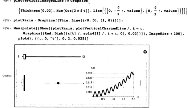
distances$x>P$_{is given}by, $E[x]=KQ_{0}$$[ 2. /i( \frac{1}{\sqrt{(x-,)^{2}+\langle\frac{6}{2})^{2}}}-\frac{1}{\sqrt{x^{2}+(\frac{\delta}{2}\rangle^{2}}}]]$. Thisisacomposite equationbasedon the fieldequation given inthepreviouscase.

Onemaywishtoplot thisfield. The codeis given;however,duetomanuscriptspacelimitation theoutpmis suppressed.

$|n[33]=$ EfieldTopBottom$[x_{-}]$ _$:=2.$ $/1( \frac{1}{\sqrt{(x-t)^{2}+(\frac{\delta}{2}\rangle^{2}}}-\frac{1}{\sqrt{x^{2}+\langle\frac{\delta}{2}\rangle^{2}}}1/$

.

values

$|\cap[34]=$ Plot[EfieldTopBottom_$[x],$ {_$x,$ $(1+0.1)$ $/$

.

values, $(i+3.0)/$

.

values},

PlQtStyle$arrow$Thick, AxesLabel $arrow\{\prime\prime x, m", /E_{-}$field, $N/C”\}$, GridLines$arrow$ Automatic];

Fortime-dependent charge $Q$asinthepreviouscase weconsider$Q(t)=Q_{0}$Cos$[2\pi ft]$. Thecorrespondingequation of

motionforacharge$q$becomes,

$|n[35]=$ eqx3 _$=x$‘ ‘

$[ t]-(\frac{kQ_{0}q}{m}1$ (EfieldTopBottom$[x]/.$ $xarrow x[t]$) Cos $[2\pi ft]//$

.

values;

Assigningasetof initial conditionswesolvetheequation numerically.

$|n[36|\circ$ solx3 $=$ NDSolve$[\{eqx3 ==0\dot{},x[O]--=0.6, x’[0]--=0\}, x[t], \{t, 0,2.0\}]$;

Utilizing the solutionweplot its kinematicsvs.time.

$|n\dot{\downarrow}37]=$ plot3 $=$Plot$[x[t]/$

.

solx3, _{$\{t, 0,2.0\}$}, PlotStyle $arrow$Thick,

AxesLabel $arrow t”t,$$s”$, “

$x,m”$}, GridLines$arrow$ Automatic, PlotRange$arrow$All];

$|n[3S]=$ {velocity3f, acceleration3f} _$=\{D[x[t]/. _{solx3, \{t, 1\}], D[x[t]/.} _{solx3, \{t, 2\}]\}$} _; $|n(39]=$ plotvelocity3f $=$Plot[velocity3f, $\{t, 0,2. \},$

PlotStyle $arrow$ {Thick, Red}, AxesLabel _{$arrow t”t,$}_$s”,$

$\prime$

(7)

RIMS Sarafian No$vember27_{-}2012.nb$

$|n\{40|=$ plotacceleration3f$=$ Plot$[$accelerat $ion3f,$ $\{t, 0;2. \},$ PlotStyl$\bullet$$arrow\{$Thick, $Gr\bullet\bullet n\},$ $lxesLabelarrow\{"t,$$s”,$ $na,m/s^{2,\prime}\}$, GrldLin$\bullet$$garrow$Automatic, PlotRange$arrow$All$]$;

$|\cap|41|--$ plotTopBottomChargedLines $:=$ Graphics$[\{$

Thickness$[0.02]$, Hu$\bullet$[Coc$[2\pi$ft$]$], Line$[\{\{0,$ $\underline{\delta}/$

.

values$\},$ $\{l/$

.

values,

$\underline{\delta}/$

.

values$\}\}],$

2 2

Thickness[O. 02], Hue$[$Cos$[2\pi St]],$

$\delta$ $\delta$

Line$[\{\{0,$

$–/.$

_$values\},$ $\{i/$

.

valu$\bullet\bullet$, -– /. $v\bullet 1u\circ e\}\}]\}]$

2 2

$|n|42|\overline{-}$ GraphicsGrid[

{{plotxllf, plot2, plot3}, {plotvelocityllf, plotvelocity2f, $plotvolocAty3f$},

{plotaccelerationllf, plotacceleration2f, $plotacc\bullet 1\bullet ration3f$}$\}$, ImageSize$arrow 500$]

$KJn$ $x,m$ x,m

$v\mu lVs vps vfls$

$Out[42]=$

$ar\int s^{2}$ a$lWs^{2}$ $arVs^{2}$

$ts$

Figure

3.

Display ofthe$\{x, v, a\}$

vs.

$t$for

case

1through 3.

Foravisual understanding

we

simulate themotion

as

wcll.

(8)

$RIMS_{-}Sarar\prime an_{-}N0$vemb$er27_{-}2012.nb$

$|n[44|=$ Nanipulate[{Show[{plotXaxis, plotTopBottomChargedLines /. $tarrow\tau,$

Graphics$[ \{ Red, Disk[\{x[t]/. solx3[1\prod/. tarrow r, 0\}, 0.02]\}]\}, lmageSizearrow 200],$

plot3}, $\{\{r, 0, /t"\}, 0,2, O.025\}]$

$\blacksquare$Case4. Weconsideraverticalchargedline. Inthisscenariocharge

$Q$is distributedevenlyon avertical lineof length$\delta.$

Theelectricfield along the symmetry axisline,$x$

.

The distanceawayfromthelineis given by,

$E[x]=KQ \frac{1}{x\sqrt{x^{2}+(\frac{\delta}{2})^{2}}}.$

$|n[45]=$ EfieldLeftVerticalLine$[x_{-}]$ $:=\underline{1}/$

.

values

$x\sqrt{x^{2}+\langle\frac{\delta}{2})^{2}}$

Ascaledplotofthefield, $\frac{1}{KQ}E(x)$ isshown; the outputis suppressed.

$|$n[4\^o]$=$ Plot[EfieldLeftVerticalLine_$[x]$, {

$x,$ $(1+O.$$1)/$

.

values, $(’+3.0)/$

.

values},

PlotStyle$arrow$ Thick, AxesLabel$arrow\{\prime\prime x, m", /E_{-}$field, $N/C”\}$, GridLines$arrow$Automaticl;

The equation of motion of the corresponding field foratime-independent field is:

$x(t)- \frac{KQq}{m}[\frac{1}{x\sqrt{x^{2}+(\frac{\delta}{2})^{2}}}]=0$. Setting $\frac{KQ_{0}q}{m}=1$following the procedure given inthepreviouscases onemay_{solve the}equation numerically. _Theexercise is left

to

theinterested of the reader. Herewesolve theequation of motion foratime-dependent oscillating charge distribution. Its

solution forasetofinitial conditionsis,

$|n[47]=$ eqx4 $=x$‘ ‘

$[ t]-(\frac{kQ_{0}q}{m}1$ (BfieldLeftVerticalLine$[x]/.$ $xarrow x[t]$) Cos$[2\pi$ft$]//$

.

values;

Utilizingthissolutionweevaluate theequationandthendisplay its kinematics.

$|n[4S]=$ solx4 $=$ NDSolve$[\{ eqx4---- 0, x[O]--=0.6, x‘[0]=_{-}^{-}0\}, x[t], \{t, 0,2.0\}]$;

$|n[49]=$ plot4 $=$Plot$[x[t]/$

.

solx4, $\{t, 0,2.O\}$, PlotStyle$arrow$ Thick,

AxesLabel $arrow t”t,$$s”$, “_$x,m”$_}, _GridLines$arrow$Automatic, PlotRange$arrow$All]

$i$

$|n[50]=$ {velocity4f, acceleration4f} _{$=\{D[x[t]/. solx4, \{t, 1\}], D[x[t]/.} _{solx4, \{t, 2\}]\}$ ;} $|n[51]=$ plotvelocity4f$=$ Plot[velocity4f, _{$\{t, O, 2.} _\},$

(9)

$RIMS_{-}Saraf\dot{/}an_{-}November27_{-}2012.nb$

$|n[S2]=$ plotacceleration4f$=$ Plot$[acceleration4f,$ _{$\{t, O, 2. \}$}, PlotStyle $arrow$ { Thick, Green},

AxesLabel$arrow\{^{\mathfrak{n}}t,$$s”,$ $\mathfrak{n}a,m/s^{2_{\mathfrak{n}}}\}$, GridLines$arrow$Automatic, PlotRange$arrow$All$]$;

$|\cap[53]=$ GraphicsGrid[{{plotxllf, plot2, plot3, plot4},

{plotvelocityllf, plotvelocity2f, plotvelocity3f, plotvelocity4f},

{plotaccelerationllf, plotacceleration2f, plotacceleration3f,

plotacceleration4f}$\}$, lmageSize$arrow 500$];

Figure4. Display of the$\{x, v, a\}$vs.$t$forcase1 through4.

Duetomanuscriptspacelimitation the graphic output is suppressed. Foravisual understandingwesimulate the motionas

well.

$|\cap|54|=$ plotVerticalChargedLine $:=$Graphics$[$

$\{Xhickness[0.02]$, Hue [Cos$[2\pi$ft$]$], Line$[\{\{0,$ $- \frac{\delta}{2}/$

.

values$\},$ $\{0,$ $\frac{\delta}{2}/$

.

values_$\}\}]\}]$

$|n[S5|^{\backslash }=$ plotXaxis $=$Graphics$[\{$rh$ln$, Line$[\{\{O,$ $0\},$ $\{1,0\}\}]\}]$;

$|n|56]=$ Manipulate$I${Show[{plotXaxis, plotVerticalChargedLine/. _{$tarrow r,$}

Graphics$[\{$Red, Disk$[\{x[t]/$

.

solx4[1] /. _{$tarrow r,$} $0\},$ $0..02]\}]\}$, lmageSize$arrow 2OO$],

plot4}, $\{\{r, 0, \mathfrak{n}t"\}, 0,2,0.025\}]$

$\oplus$

$Out\iota 56|=$

$1$

$–$ $-$–

$\blacksquare$Case5. We consider

a

horizontallydisplaced vertical line charge distribution. The physics of this

case

is similartoCase

4. Inthisscenariothe vertical chargeslidesalongthe$x$-axisby

a

length$f$. Replacing$x$with$x-l$inthefieldequationof

Case4yieldsthe neededfieldforthe

case

athand.

$|n[s\eta_{r}$ ZfieldRightVerticalLine$[x_{-}]$ $:=1/(( x-\sqrt{})\sqrt{}((x-t\rangle^{2}+(\frac{\delta}{2})^{2}))/$

.

values

$|n[S8)z$ Plot [EfieldRightVerticalLine $[x],$ {$x,$ $(’+O.$$1)/$

.

values, $(/+3.O)$ $/$

.

values},

PlotStyle $arrow$Thick, AxesLabel$arrow t”x,$$m”$, “$B_{-}$field, $N/C^{\mathfrak{n}}$}, GridLines$arrow$ Automatic];

The correspondingequation of motion foratime-dependent charge distributionis,

$|n[\S 9]=$ eqx5 $=x$ ‘ ‘ _{$[ t]-(\frac{kQ_{0}q}{m}1$} _{(ZfieldRightVerticalLine}_$[x]/.$ _{$xarrow x[t]$}₎ _Cos_$[2\pi$_ft_$]//$

.

_values;

Thenumeric solution of this equation forasetof initial conditions yieldsthekinematics ofthecharge$q.$

(10)

$RIMS_{-}Sarar/an_{-}November27_{-}2012.nb$

$|n[61]=$ plot5 $=$ Plot$[x[t]/$

.

solx5, $\{t, 0,2.O\}$, PlotStyle$arrow$ Thick,

AxesLabel$arrow t”t,$$s”$, “_$x,m”$_}, _GridLines

$arrow$Automatic, PlotRange$arrow$All];

$|\cap[62]=$ {velocity5f, acceleration5f} $=\{D[x[t]/. solx5, \{t, 1\}], D[x[t]/. solx5, \{t, 2\}]\}_{i}$

$|n[63]=$ plotvelocity5f$=$ Plot[velocity5f, $\{t, 0,2. \}$, PlotStyle $arrow$ {Thick, Red},

AxesLabel $arrow\{/t, s", " V;^{m/s"}\}$, GridLines$arrow$Automatic, PlotRange$arrow$All]

$i$

$\ln\{64_{}1=$ plotacceleration5f$=$ Plot$[$acceleration$5f,$ $\{t, 0,2. \}$, PlotStyle $arrow$ {Thick, Green},

AxesLabel$arrow\{\prime\prime t,$$s”,$ ‘a,m$/s^{2_{\mathfrak{n}}}\}$, GridLines$arrow$Automatic, PlotRange$arrow$ All$]$;

$|\cap[65]=$ GraphicsGrid[{{plotxllf, plot2, plot3, plot4, plot5},

{plotvelocityllf, plotvelocity2f, plotvelocity3f, plotvelocity4f, plotvelocity5f},

{plotaccelerationllf, plotacceleration2$f$, plotacceleration3$f,$

plotacceleration4f, plotacceleration5f}$\}$, lmageSize$arrow 800$]$i$

Figure5. Displayof the$\{x, v, a\}$vs.$t$forcase1 through 5.

Duetomanuscriptspace limitationthegraphicoutputis suppressed.

$\blacksquare$Case6. Weconsidertwoverticalparallel charged lines. We

combine thefieldsofCase 4and5. The code todisplaythe

corresponding field is given;itsoutputis suppressed.

$|n[66|=$ Plot[EfieldLeftVerticalLine$[x]+$EfieldRightVerticalLine$[x],$

{$x,$ $(i+0.1)/$

.

values, $(’+3.0)$ $/$

.

values}, PlotStyle$arrow$ Thick,

AxesLabel$arrow\{\prime\prime x, m\mathfrak{n}, /E_{-}$field, $N/C”\}$, GridLines $arrow$Automatic];

Theequationof motion,its solution andrelatedkinematicsare,

$|n[67]=$ eqx45$=$

$x$‘ ‘ $[ t]-(\frac{kQ_{0}q}{m})$ ((EfieldLeftVerticalLine[x] $+$BfieldRightVerticalLine$[x]$) $/.$ $xarrow x[t]$)

Cos $[2\pi ft]//$

.

values;

$|n[68|=$ solx45 $=$ NDSolve$[\{eqx45 ----0, x[O]----0.6, x’[0]=_{-}^{-}0\}, x[t], \{t, O, 2.O\}]$ ;

$|n[69]=$ plot45 $=$ Plot$[x[t]/$

.

solx45, $\{t, O, 1.0\}$, PlotStyle$arrow$ Thick,

AxesLabel$arrow t”t,$$s”,$ $\prime\prime x,$$m”$}, GridLines $arrow$Automatic, PlotRange$arrow Al1$];

$|n[70]=$ {velocity45f, acceleration45f} _{$=\{D[x[t]/. solx45, \{t, 1\}], D[x[t]/.} _{solx45, \{t, 2\}]\}_{i}$} $|n[71]=$ plotvelocity45f $=$ Plot[velocity45f, $\{t, 0,2. \}$, PlotStyle$arrow$ {Thick, Red},

AxesLabel$arrow t”t,$$s”$, “_$v,m/s”$_{}, GridLines}

$arrow$Automatic, PlotRange$arrow$All];

$|n[72]=$ plotacceleration45f$=$ Plot$[$acceleration$45f,$ _{$\{t, 0,2.} _\}$, PlotStyle$arrow$ {Thick, Green},

AxesLabel$arrow\{"t,$$s”,$ $/a,m/s^{2,\prime}\}$, GridLines$arrow$Automatic, PlotRange$arrow$ All$]$;

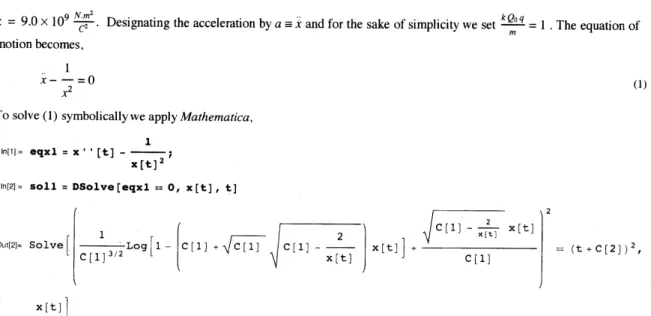
$|n[73]=$ GraphicsGrid_[{{plotxllf, plot2, plot3, plot4, plot5, plot45},

{plotvelocityllf, plotvelocity2f, plotvelocity3f, plotvelocity4f, plotvelocity5f, plotvelocity45f}, {plotaccelerationllf, plotacceleration2f, plotacceleration3f,

plotacceleration4f, plotacceleration5f, plotacceleration45f}$\}$, ImageSize$arrow 800$];

Duetomanuscriptspacelimitation the graphic output is suppressed.

Figure6. Displayof the$\{x, \nu, a\}$vs.$t$forcase1 through5.

$\blacksquare$Case 7. We considerahorizontalone-end-closed one-end-open rectangular

chargedbox. Thisscenari$0$isgeneratedby

(11)

$RIMS_{-}S arafia\bigcap_{-}November27_{-}2012.nb$

The plotcodefor the electric field isgiven,and its output issuppressed.

$|n|74]=$ Plot [!fieldTopBottom$[x]+$BfieldLeftVerticalLine[$x],$

$\{x,$ $(’+0.1\rangle/.$ values, $\langle’*3.0)$ $/$

.

values$\}$, PlotStyl$\bullet$$arrow$rhick,

AxesLabel$arrow\{"x,m",$ $\prime\prime Z_{-}$field, $N/C”\}$, GridLines $arrow$Automatic];

$|\cap \mathfrak{l}75]_{\Xi}$ eqx34 $=x$‘ ‘$[ t]-(\frac{kQ_{0}q}{m}1$

$((BfieldTopBotto\varpi[x]+$BfieldLeftVerticalLine[$x])/. xarrow x[t])$ Cos$[2\pi ft]//$

.

values;

$|n[76|=$ solx34$=$ NDSolve$[\{eqx34---- 0, x[O]\overline{-}--0.6, x ‘ [0]=_{-}^{-}0\}, x[t], \{t, 0,2.O^{-}\}]i$

$|n[77]=$ plot34 $=$ Plot$[x[t]/$

.

solx34, $\{t, 0,2.0\}$, PlotStyle$arrow$rhick,

AxesLabel$arrow\{\prime\prime t, s", /x, m"\}$, GridLines $arrow$Automatic, PlotRange$arrow$ All]$i$

$\ln[7S]=$ {velocity34f, acceleration34f} $=\{D[x[t]/. solx34, \{t, 1\}], D[x[t]/. solx34, \{t, 2\}]\}_{i}$ $|n|79|=plotv\bullet locity34f=$ Plot[velocity34f, $\{t, 0,2. \}$, PlotStyle $arrow\{$Bhick, Rod$\},$

AxesLabel $arrow\{\prime\prime t, s", /v,m/s^{\mathfrak{n}}\}$, GridLines$arrow$Automatic, PlotRange$arrow$All]$i$

$|n|S0]=$ plotacceleration34f$=$ Plot$[accel\bullet ration34f,$ $\{t, 0,2. \}$, PlotStyle $arrow$ {Thick, Green},

AxesLabel $arrow\{\prime\prime t,$$\epsilon",$

$\mathfrak{n}$

a,m$/s^{2,\prime}\}$, GridLines$arrow$ Automatic, PlotRange$arrow$All$]$;

$|n[S1]=Graphlc\epsilon Grid$[{{plotxllf, plot2, plot3, plot4, plot5, plot45, plot34},

{plotvelocityllf, plotvelocity2f, plotvelocity3f,

plotvelocity4f, plotvelocity5f, plotvelocity45f, plotvelocity34f},

{plotaccelerationllf, plotacceleration2f, plotacceleration3f, plotacceleration4f,

plotacceleration5f, plotacceleration45f, $plotaccoleration34f$}$\}$, lmageSize$arrow\epsilon oo$] ;

Duetomanuscriptspacelimitation the graphic output is suppressed.

Figure7. Display of the$\{x, v, a\}$

vs.

$t$for

case

1 through6.

For

a

visual understanding

we

simulateth$e$motion

as

well.

$\ln|S2]=$ plotRotatedCup $:=$Graphics$[\{$Thickness[O.02],

Hue[Cos$[2\pi$ft$]$], Line$[\{\{0,$ $- \frac{\delta}{2}/$

.

values$\},$ $\{t/$

.

values, $- \frac{\delta}{2}//$

.

values$\}\}],$

Thickness[0.02], Hue[Cos$[2\pi$ft$]$],

Line$[\{\{0,$ $\underline{\delta}/$

.

values$\},$ $\{l/$

.

values, $\underline{\delta}/$

.

values$\}\}],$ 2 2

Thickness$[O. 02]$, Hue$[$Cos$[2\pi ft]]$, Line$[\{\{0,$ $- \frac{\delta}{2}/$

.

values$\},$ $\{0,$ $\frac{\delta}{2}/$

.

values_$\}\}]\}]$

(12)

$RIMS_{-}Sara\Gamma/an_{-}No$vemb$er27_{-}2012.nb$

$|n[84|=$ Nanipulate$[\{$Show$[\{$plotXaxis, plotRotatedCup _/. $tarrow\tau,$

Graphics$[ \{Red, Disk[\{x[t]/. solx34[1\prod/. tarrow\tau, 0\}, 0.02]\}]\}, lmageSiaearrow 200],$

plot34}, $\{\{\tau, 0, /t"\}_{t}0,1.2, 0.025\}]$ $0$ $1$ $Out[S4]=$ 0.5 10 $1S$ 2.0 $\wedge\cdot$–

Figure$7a$

.

Schematicof theone-end-closed one-end-open_rectangular_{charge distribution}_(left_graph),_and_positionvs._time

(right graph).

$\blacksquare$Case8. We consideracharged rectangular closed box. By combining the configurations of Case 3,

4and5

we

arriveat

the field of

a

rectangularcharged distribution. Asin thepreviousscenarios the relevant associated information yields,

$|n[S5]=$ Plot[EfieldTopBottom_$[x]+$EfieldLeftVerticalLine_$[x]+$EfieldRightVerticalLine_$[x],$

{$x,$ $(1+0.1)/$

.

values, $(1+3.0)/$

.

values}, PlotStyle$arrow$Thick,

AxesLabel$arrow t”x,$$m”$, “$E_{-}$field, $N/C”$}, GridLines$arrow$Automatic];

$|n|S6|=$ eqx345 $=x$“

$[t]-(\underline{kQ_{0}q}m)$

((EfieldTopBottom$[x]+$EfieldLeftVerticalLine$[x]+$EfieldRightVerticalLine$[x]$) $/.$

$xarrow x[t])$ Cos$[2\pi$_ft$]//$

.

values;

$|n[s\eta=$ solx345 $=$ NDSolve$[\{eqx345 =_{-}^{-}0, x[0]----O. 6, x’[0]--=0\}, x[t], \{t, 0,2. O\}]i$

$|n[8S|=$ plot345 $=$Plot$[x[t]/$

.

solx345, $\{t, 0,0.8\}$, PlotStyle$arrow$Thick,

AxesLabel $arrow t”t,$$s”$, “

$x$,m’1}, GridLines $arrow$Automatic, PlotRange$arrow$All];

$|n[S9]=$ {velocity345f, acceleration345f} $=\{D$[$x[t]/$

.

solx345, $\{t,$ $1\}$], $D$[$x[t]/$

.

solx345, $\{t,$ $2\}$]$I$;

$|n[90]=$ plotvelocity345f $=$ Plot[velocity345f, _{$\{t, 0,2.} _\}$, PlotStyle$arrow$ {Thick, Red},

AxesLabel$arrow\{\prime\prime t, s", /v,m/s^{\mathfrak{n}}\}$, GridLines$arrow$ Automatic, PlotRange$arrow$All];

$|n[91]=^{-}plotacceleration345f=$ Plot$[$acceleration345f, _{$\{t, 0,2.} _\}$, PlotStyle$arrow$ {Thick, Green},

AxesLabel$arrow\{\prime\prime t,$$s”,$ $/a,$$m/s^{2,\prime}\}$, GridLines$arrow$Automatic, PlotRange$arrow$All$]$;

$|n[92]=$ GraphicsGrid_[{{plotxllf, plot2, plot3, plot4, plot5, plot45, plot34, plot345},

{plotvelocityllf, plotvelocity2f, plotvelocity3f, plotvelocity4f,

plotvelocity5f,

$plotvel$

, plotvelocity34f, plotvelocity345f},

{plotaccelerationllf, plotacceleration2f, plotacceleration3f,

plotacceleration4f, plotacceleration5f, plotacceleration45f,

plotacceleration34f, plotacceleration345f}$\}$, lmageSize$arrow 800$];

(13)

$RIMS_{-}Sara\Gamma\prime an_{-}No$vemb$er27_{-}2012.nb$

$|n[93)=$ plotRectangularBox $:=$ Graphics$[\{$Thickness$[O. 02],$

Hue[Cos$[2\pi$ft$]$], Line$[\{\{0,$ $- \frac{\delta}{2}/$

.

values$\},$ $\{t/$

.

values, –$\frac{\delta}{2}/$

.

values$\}\}],$

Thickness$[O. 02]$, Hue[Cos$[2\pi$ft$]$],

Line$[\{\{0,$ $\underline{\delta}/$

.

values$\},$ $\{t/$

.

values, $\underline{\delta}/$

.

values$\}\}],$ 2 2

Thickness[0.02], Hue [Cos$[2\pi$ft$]$], Line$[\{\{0,$ $-\underline{\delta}/$

.

values$\},$ $\{0,$

$\underline{\delta}/$

.

values$\}\}]t$

2 2

Thickness[0.02], Hue$[$Cos$[2\pi ft]],$

Line$[\{\{t/.$ $values_{t}-\frac{\delta}{2}/$

.

values$\},$ $\{1/$

.

values, $\frac{\delta}{2}/$

.

values$\}\}]\}]$

plotXaxis $=$Graphics$[\{Thin$, Line$[\{\{O,$ $0\},$ $\{1$, $0\}\}]\}]$;

Manipulate$[\{$Show$[\{$plotXaxis, plotRectangularBox /. $tarrow\tau,$

Graphics$[ \{Red, Disk[\{x[t]/. solx345[1\prod/. tarrow r, 0\}, 0.02]\}]\}, lmageSiaearrow 200],$

plot345}, $\{\{r, 0, /t"\}, O, O. 28,0.025\}]$

$\blacksquare$Summary andConclusions

Itistheobjective ofthisarticletodemonstrate byutilizingaComputer Algebra System(CAS),particularly Mathematicaon$e$

maydeviate fromthetraditionalrouteofsolvingproblems. The ultimate objective ofaphysics research project isthe output

of theanalysis and Mathematica providesonesuch innovative approach. The traditional approachtosolve,a

mathematical-physics problem inmostscenariosencounterssolving complicatedequationsanalytically. One devotesconsiderableefforts

doing

so

and failsinmost

cases.

This derails thefocus

on

theobjectives. The authorbelievesCAS andparticularly

Mathe-matica isanalternative effective approach. The examples shown in this article demonstrate how effectively

one can

focus

on

the objectives of the proposed problems and convenientlywithoutdistraction achieve thesetgoals. Theexamplesarechosen

from electromagnetismand theproposed approach easilymay be appliedtoother fields of interest. Also it isworthwhile

pointingoutthattheentire manuscriptincludingtext,symbolic and numeric computations,tables,andgraphsareembodied

inonesinglefile. Thisby itself isatremendous advantageassistingtoavoidcompiling multiple individualfiles.

$\blacksquare$Acknowledgement

Theauthor is gratefultothechair of the organizerofthe Researeh Institute for Mathematical Sciences Symposium, Professor

Yasuyuki Nakamura-san for inviting himtopresent this article. He isalsothankful forthefinancial support of the RIMSof

Kyoto University, Japan. The paperspresentedatthesymposium wereinformative and stimulating. Theauthor isecstatic

(14)

$RIMS_{-}S ara\Gamma ja\bigcap_{-}November27_{-}2012.nb$

theoretical physics,atthe Center for TheoreticalPhysics/KyotoUniversity

on

August 22,2012.

$\blacksquare$ References

[1]MathematicaV 8.04,Wolfram Research Inc.

[2]Halliday, ResnickandWalker,“Fundamentals of Physics”, 8thedition,John Wiley andSons,Inc.2008.

Reitz andMilford,“Foundations of Electromagnetic Theory”, Addison-Wesley Publishing Company, Inc. 1960