A modified pattern matrix algorithm for multichain MDPs(The Development of Information and Decision Processes)

A

modified

pattern matrix

algorithm

for multichain

MDPs

宮崎大学・教育文化学部 伊喜哲–郎 (Tetsuichiro IKI)

Faculty

_of

Education and Culture, Miyazaki University

弓削商船高等専門学校・総合教育科 堀口正之 (Masayuki HORIGUCHI)

General Education, Yuge National College

_of

Maritime Technology

Abstract

A pattern matrix algorithrn for niultichain Markov decision processes wvith

average

criteria proposed in our $\mathrm{p}\mathrm{r}e$vious work[10] will be modified by iise of

the so-called vanishing discount approach by letting $\tauarrow 0$ for the $(1-\tau)$

discount

case.

Keywords: multichainMarkov decision processes,

average

reward structured

algorithni, comlnunicating

_class.

transient class, value iteration, _vanishing

dis-count approach.

1

Introduction and notation

In this paper, we are concerned with the structured pattern matrix algorithm for

mul-tichain finite state $\sim 1\backslash \prime \mathrm{I}\mathrm{a}\mathrm{l}\mathrm{k}\mathrm{o}\mathrm{v}$ decision processes (MDPs)

with an

average

rewardcriterion.

The efficient algorithm for findillg an optimal policy in average reward MDPs have been

studied by $\mathrm{n}\mathrm{l}\mathrm{a}\mathrm{n}]^{\gamma}$ authors (cf. [5, 9, 13.

14.

15, 19]). For the unichain

or

communicating

case, the optimal policy can be found by solving a singleoptimalitv equation (cf. [15]).

However, _{for the multichain case, the optimal policy is characterized by two equations,}

called the multichain optimality equations, which are solved, for example, by linear pro-gramming (cf. [6, 15])

or

policy iteration algorithms (cf. [7, 9, 15]).

The valueiteration method based on classificationofthestate spaceinto closed

com-municating subsets and transient

one

has been given by Schweitzer[17] and $\mathrm{O}\mathrm{h}\mathrm{n}\mathrm{o}[14_{\rfloor}^{\rceil}$.

$\mathrm{O}\mathrm{h}\mathrm{n}\mathrm{o}[14]$ has given the stopping rule to find an $\underline{c}$-optilnal policy in a finite number

it-erations using by Schweitzer’s value iteration method. Recently, Leizarowitz[13] has

ex-tended the above algorithm tothe caseofcompactstate space. In

our

previous work[10],

we

have proposed an algorithm for the multichain finite state MDPs in which the state

$(^{\circ 1\dot{r}\mathrm{h}_{\iota}^{\backslash }\backslash ^{\backslash }\mathrm{i}\mathrm{f}\mathrm{i}\mathrm{c}_{C}^{i}\iota \mathrm{t}\mathrm{i}\mathrm{c})\mathrm{n}}‘$, is

$(1_{011(}, 1y.)^{r}$ use of$\mathrm{t}$}

$\iota(’((\mathrm{r}\mathrm{r}\mathrm{t}_{\mathrm{b}1)(11(1\mathrm{i}\mathrm{n}\mathrm{g}\iota)_{C}\iota\uparrow \mathrm{t}\mathrm{t}’ 1\mathrm{n}\mathrm{I}\mathrm{n}\mathrm{a}\mathrm{t}\mathrm{l}\mathrm{i}\mathrm{c}\cdot \mathrm{e}\mathrm{s}^{\backslash }}^{\Delta\backslash }\cdot$ and the idea ofvalue

iteration algorithm. $\mathrm{H}\mathrm{o}\backslash ,\backslash \cdot \mathrm{e}\mathrm{t}^{r}\mathrm{e}\mathrm{r}$ , the finding of an optimal

policy for each communicating subset is supposed to

use

the policy improvement.

The

_ob.iective

of this paper is to propose the modified algorithm in which, to obtain

an optimal policv for each communicating $\mathrm{c}1\sigma\backslash \mathrm{S}_{\iota}\mathrm{S}$

.

weuse the

so-called vanishing discount approach by considering the corresponding $(1-\tau)$ discountedexpected reward

as

letting $\tauarrow 0$

.

In the rerninder of this section, _{we will define finite state INIDPs to be exaniined and}

describe the basic results for the average and discounted

case.

We define a controlled $\mathrm{d}\backslash .\cdot \mathrm{n}\mathrm{a}\mathrm{m}\mathrm{i}\mathrm{c}$ system with a finite state space denoted bv $S=$

$\{1,2, \ldots.\wedge’\backslash ^{\mathcal{T}}\}$. Associatedwith eachstate $i\in S$ is a non-emptyfinite set.4(i) of available

moves

to

a

new state $j\in S$ with probability ($\mathit{1}ij(a)$ where _{$\sum_{j\in S}q_{ij}(a)=1$} for all $i\in S$

and $a\in A(?)$ and the reward $r(\dot{r,}\mathit{0})\}$ is earned. The process is repeated from the new

state $j\in S$. This structure is callOd a Markov decision process. denoted by an MDP

$\Gamma=$ _{$(S, \{.4(\prime i) : i\in S\}.Q, r)$}. where $Q=(q_{\mathrm{i}j}(a) : i.j\in S.\mathit{0}\in A(i))$ and $r=r(i, a)\in \mathbb{R}$

for all $i\in S$ and $a\in A(i)$ and $\mathbb{R}$ is the set of all real numbers. The set of

admissible

state-action pairs will be denoted })$\}^{r}$

$\mathrm{K}=\{(i, a) : i_{l}\in S, \mathit{0}_{}\in A(i)\}$.

The sample space is the product space $\Omega=\mathrm{K}^{\infty}$ such that the projection _{$(X_{t}, \Delta_{t})$}

on

the

t-th factor describesthe state and action at the t-th time oftheprocess $(t\geqq 0)$

.

A policy

$\pi=$ $(\pi_{0},$$r_{1\mathrm{l}}$,

. .

.

$)$ is

a

sequence ofconditionalprobabilitieswith$\pi_{t}(A(x_{t})|x_{0}, a_{0}, \ldots , x_{\ell})=1$

for all histories $(x_{0}.a_{0}, \ldots , x_{t})\in \mathrm{K}^{t}S(t\geqq 0)$ where $\mathrm{K}^{0}S=S$

.

The set of all policies is

denoted by $\Pi$. A policy _{$\pi=(r_{10}.\pi_{1}, \ldots)$} is called randomized stationary ifa conditional

probability $\gamma=$

, $(\gamma(\cdot|i) : i\in S)$ given $S$ exists. for which $\pi(\cdot|.\tau_{\mathit{0}}, a_{0}, \ldots, x_{t})=\gamma(\cdot|x_{t})$ for all $t\geqq 0$ and $(.r_{0}.\mathit{0}_{0}, \ldots.x_{t})\in \mathrm{K}^{r,}S$

.

Such

a

policy is simply denoted by

$\gamma$

.

We denote by $\Gamma^{d}$ the set of functions

on

$\mathrm{S}$

with $f(\prime i)\in A(i)$ for all $i\in S$

.

A randomized stationarv

policy $\wedge$

,

is called stationary if there exists

a

function

$f\in F$ such that $\gamma(\{f(i)\}|i)=1$

for all $i\in S$, which is denoted simply by $f$. For each $\pi\in\Pi$_, starting state _{$X_{0}=i$}, the

probability

measure

$P_{\pi}(\cdot|X_{0}=\dot{\tau})$ on $()$ is defilied in a usual way. The

$1$)

$\mathrm{r}\mathrm{o}\mathrm{b}\mathrm{l}\mathrm{e}\mathrm{I}\mathrm{l}\mathrm{l}$ we are

concerned with is the lnaximization of the long-run expected

average

reward per unit

time, which is defined by

(1.1) $\mathrm{U}^{f}(\prime i, \pi)=\varliminf_{T}\inf_{\infty}\frac{1}{\prime\tau}E_{\pi}(\sum_{t=0}^{T-1}r(\swarrow \mathrm{Y}_{t}, \triangle_{t})|X_{0}=?)$ ,

where $E_{\pi}(\cdot|_{z}\mathrm{Y}_{0}=i)$ is the expectation w.r.t. $P_{\pi}(\cdot|X_{0}=\prime i)$

.

A policy $\pi^{*}\in \mathrm{I}\mathrm{I}$ satisfying tlrat,

(1.2) $?l’(i, \pi^{*})=\mathrm{s}\mathrm{u}\mathrm{p}\nu’(i, \pi)\pi\in\Pi:=\psi^{*}(i)$ for all $i\in S$

is called to be average optimal

or

siniply optimal.

The structured algorithm treated with in this paper is based on

a

comlnunicating model introduced by Bather[l]. $\iota,\backslash ^{\tau}\prime \mathrm{e}$ say that the MDP $\Gamma$ is communicating if ther

$e$

exists a randomizcd stationary policy $\wedge.’/=(\wedge,\langle\cdot|i)$ : $’\in S$) satisfying that the transition

matrix$Q(\gamma’)$ induced by 1 defines a irreducibleMarkov chain where $Q(\gamma^{J})=(q_{?j}.(\gamma))$ with

$q_{ij}( \wedge/))=\sum_{\mathit{0}\in A(ij^{\backslash }}q_{ij}(a)_{i}\wedge(a|i,)$ for all $i,$$j\in S$

.

Let $l?(S)$ be the set of all function

on

S.

The following fact is well known.

Lemma 1.1 (cf. _{[15]). Suppose that there exists} a constant$g$ and

a

$\iota’\in B(S)$ such that

(1.3) $\mathit{1})i=0\Leftarrow-\prime 4(i)\mathrm{n}\mathrm{u}\mathrm{a}\mathrm{x}\{r(?,, a)+\sum_{j\in S}q_{ij}(\zeta\iota)v_{j}\}-g$

for

all $i\in S$.

Then.

$g$ is unique and $g=\iota^{\prime\prime^{*}}(’.i)=\mathrm{t}^{f^{*}(i,f)}$,

for

all $i\in S$, where $f(\prime i)$ is a maximizer in

The expected total $(1-\tau)$-discounted reward is defined by

(1.4) $\mathrm{t}_{\mathcal{T}}(i, \pi)=E_{\pi}(\sum_{t=0}^{\infty}(1-\tau)^{t}r(-\mathrm{Y}_{t}, \triangle_{t})|X_{0}=?)$ for $\dot{?}\in S$ and $r_{1}\in\Pi$,

and $?_{\mathcal{T}}’( \prime i)=\sup_{\pi\in \mathrm{n}’}\iota f_{\mathcal{T}}(i, \pi)$ is called a $(1-\tau)$-discounted value function, where $(1-\tau)\in$

$(0,1)$ is a given discount factor.

For

any

$\tau\in(0,1_{\text{ノ}^{})}$

.

$\mathrm{w}\mathrm{t}^{i}$ define the operator $C_{\tau}^{\tau}$,

:

$B(S)arrow B(S)$ by

(1.5) $U_{\tau}u(i)= \mathrm{n})\mathrm{a}\mathrm{x}a\in.4\{r\cdot(i.a)+(1-\tau)\sum_{j\in S}q_{ij}(a)v(j)\}$ for all $i\in S$ and _{$u\in B(S)$}.

KVe have the following.

Lemma 1.2 ([15]). It holds that

(i) the operator $U_{\tau}$ is

a

contraction with the modulus $(1-’\sim)$ and

(ii) the $(1-\tau)$-discount value$f\dot{u}$nction $varrow(i)$ is a uniqzte

fixed

point

of

$L/_{\tau}^{7},\cdot i.e.$,

(1.6) $’\iota J_{\tau}=U_{\tau}v_{\mathcal{T}\}$

(iii) $\iota_{\tau}’(i)=v_{\tau}(i.f_{\tau})$ and $\varliminf_{\tau 0}\tau\iota_{\tau}’(i)=\iota_{\mu^{*}}^{J}’(i)$, where $f_{\tau}$ is a maximizer

of

the right-hand

side in $(\mathit{1}.\theta)$.

In Section 2, _{the methodsofclassifying the set of}states by

use

of t.he corresponding

pattern matricesis proposed. whichis used tofindanoptimalpolicy bythevalueiteration algorithm in Section 4. In section 3, an optimal policy for each communicating class is obtained bv use of the vanishing discount, _{approach by letting} $\tauarrow 0$. In Section 5,

a

$\mathrm{n}\iota 1\mathrm{m}\mathrm{e}\mathrm{r}\mathrm{i}\mathrm{c}^{i}\mathrm{d}_{}1$example is given to comprehend our structured algorithm.

2

Classification

of the

states

In this section, $\mathrm{f}\mathrm{i},\mathrm{o}\mathrm{m}$ our previous $\mathrm{w}\mathrm{o}\mathrm{r}\mathrm{k}[10_{\dot{\mathrm{J}}}^{1}$we quote the method of$\mathrm{c}\mathrm{l}\mathrm{a}\mathrm{S}\mathrm{S}\mathrm{i}\mathrm{b}^{r}$ing the state

space and finding the maximumsub-MDPsbyuseofthe corrpsponding pattern matrices.

whose idea is essentially the

same

as

$[13, 17]$.

For

a

non-emptv subset $D$ of S. if, for each $i\in D.$ there exists

a

non-empty subset

$\overline{A}(;i)\subset A(i)$ with_{$\sum_{j\in D}q_{ij}(a)=1$} for all $a\in\overline{.4}(i)$.

we

canconsider thesub-MDPwith the restricted state space $D$ and available action

space

$\overline{A}(i)$ for $i\in D$, which is denoted by

$\overline{\Gamma}=(D,$ $\{\overline{A}(i_{J}^{\backslash } : i\in D\}.Q_{D}.r_{D})$ where $Q_{D}$ and $r_{D}$

are

restriction of $Q$ and $r$

on

{

$(i.a)$ :

$i\in D,$$a\in$ A$(\prime i)\}$. For any$\mathrm{s}n\mathrm{b}-\backslash \mathrm{A}\mathrm{I}\mathrm{D}\mathrm{P}\overline{\Gamma}=(O. \{\overline{.4}(i) :i\in D\}.Q_{D}.r_{D})$ .

a

non-emptysubset $\overline{D}$

of$D$ is

a

communicating class in$\overline{\Gamma}\mathrm{i}\mathrm{f}\overline{D}$ isclosed, that is.

$\sum_{j\in\overline{D}}q_{ij}(a)=1$ for all$i\in\overline{D}$

and $\mathit{0}\in\overline{\wedge 4}(i)$ and the sub-MDP $(\overline{D}’.\{\overline{A}(i) :i\in\overline{D}\}, Q_{\overline{O}}, r_{\overline{D}})$ is communicating. Also,

$\overline{D}$

is maximum communicating class ifit is

not

strictlv contained in

anv

communicating

For allv positive intcger $l$

.

let $\mathbb{C}^{t}$ alld $\mathbb{C}^{l\cross l}$

be the sets of $l$-dimensional row vectors and $l\cross \mathit{1}$ matrices with _$\{0,1\}$-valu$e\mathrm{d}\mathrm{e}\mathrm{l}\mathrm{e}\mathrm{m}\mathrm{e}\mathrm{n}\mathrm{t}_{\mathrm{S}_{)}}$ respec,tively. The srum $(+)$ and product

(. operators among elements in $\mathbb{C}^{l}$ and $\mathbb{C}^{l}$xi is dePned by

$a+b= \max\{\mathit{0}_{\mathit{1}}.b\}$ and $a\cdot l$₎ $=$ $\min\{0, b\}$ for $a.b\in\{0.1\}$.

For each $i\in S$ and ($l\in A$, we define $m_{i}(a)=(\gamma\gamma\iota_{i1},(a)$

.

$r)\iota_{i2}(a)\ldots.,$$m_{iN}(a)$) $\in \mathbb{C}^{N}$ by

$(_{\backslash }2.1)$ $m_{ij}(a)=\{$

1 if $q_{ij}(a)>0$,

$0$ if _{$q_{ij}(a)=0$,}

$(j\in S)$

.

For

a

sub-MDP $\overline{\Gamma}=$

$(D, \{\overline{A}(\prime i) : i\in D\}, Q_{D}, r_{D})$ with $D=\{i_{1}, i_{2}, \ldots , i_{l}\}$

.

we

put

$m_{i}( \overline{\Gamma})=(m_{ii_{1}}(\overline{\Gamma}).m_{ii_{2}}(\overline{\Gamma}), \ldots .m_{ii_{l}}(\overline{\Gamma}))=\sum_{a\in\overline{A}(i)}m|(a|\overline{\Gamma})(i\in D)$_, where $m_{\dot{\mathrm{t}}}(a|\overline{\Gamma})=$

$(m_{ii}, (a).m_{ii_{2}}(a),$ $\ldots.m$_ii,$(a))(i\in D, a\in\overline{A}(i))$. Using $r|\iota_{i}(\overline{\Gamma})(i\in D)$, we define a pattern matrix $\mathit{1}\lambda\prime I(\overline{\Gamma}_{\mathit{1}}^{\backslash }$ for the sub-LIDP

$\overline{\Gamma}$

by

(2.2) $\Lambda^{;}I(\overline{\Gamma})=\in \mathbb{C}^{l\mathrm{x}l}$.

We note that for $i_{!}j\in D.$ $m_{\dot{\tau}j}(\overline{\Gamma})=1$

means

that there exists $0\in\overline{A}(i)$ with _{$q_{i.i},(a)>0$}

.

The pattern matrix defined above is called a communication matrix (cf. [13]).

How-ever, $\mathrm{s}\mathrm{i}\mathrm{n}\mathrm{c}\mathrm{e}_{-}\prime \mathrm{t}\prime I(\overline{\Gamma})$ determines the behaviour patternof the$\mathrm{s}\mathrm{u}\mathrm{b}- \mathrm{M}\mathrm{D}\mathrm{P}\overline{\Gamma}$

,

we

call it

a

pattern matrix in this paper. For the pattern matrix $-1\prime \mathit{1}(\overline{\Gamma})$. we define$\overline{\Lambda I}(\overline{\Gamma})\in \mathbb{C}^{l}$xi by

(2.3) $\overline{\mathit{1}1\prime I}(\overline{\Gamma}^{\backslash },\{=\sum_{k=1}^{N}M(\overline{\Gamma})^{k}$ .

Then.,

we

have the following.

Lemma 2.1. For a $r\iota on$-empty subset$\overline{D}$

of

$D,$ $\overline{D}$

is a $c\mathrm{o}7nrnunicating$ class

if

and only

if,

_for

each $i\in\overline{D}$.

$\overline{m_{ij},}(\overline{\Gamma})=\{$

1

_if

$j\in\overline{D}$, $0$ $ij$. $j\not\in\overline{D}$.

$u_{\vee}’ here\overline{rrt_{}},j(\overline{\Gamma})$ is the (i..j) element

of

$\overline{i1f}(\overline{\Gamma})$ and$\overline{.\prime\lambda\prime I}(\overline{\Gamma})=(\overline{m}_{ij}(\overline{\Gamma}))$

.

By reorderingthe states in $D,$ $\overline{\mathrm{a}\mathfrak{h}_{\text{ノ}}I}(\overline{\Gamma})$ can be transformed to the standard form:

(2.4) $\overline{:\mathrm{t}\text{ノ}f}(\overline{\Gamma})=$ $(d\geqq 1)$

.

where $E_{j}$ is a square matrix whose elements

are

all 1 $(1 \leqq.i\leqq d)$ and $[RK]$ does not

include a sub-matrix having the above form.

For any sets U. $V$, if $U\cap \mathrm{I}^{r}J=\emptyset$,

we

writ_$e$ the union _{$U\cup V$} by $U+l$

.

Here, we get the classification $0_{1}^{\mathrm{f}}$the

Theorem 2.1. For a sub-MDP $\overline{\Gamma}=$ _{$(D, \{\overline{A}(i) : i\in D\}iQ_{D}.r_{D})$}

, the state space $D$ is

$/il_{c}assif\iota’ e,d$ as

follows:

(2.5) $D=U_{1}+U_{2}^{r}+\cdots+U_{d}+L(d\geqq 1)$,

$\tau\iota_{/}’ here,$ $U_{j}i,.\mathrm{s}$ a communicating class

for

$\overline{\Gamma}(1\leqq j\leqq d)$ and $L$ is not closed.

The algoritllm of obtaining the state-decomposition (2.5) through (2.4) by tise of the

patt$e\mathrm{r}\mathrm{n}$ matrix will be called Algorithm A.

XVhen the not-closed class $L$ in (2.5) is non-empty, we go on with the state

classifica-tion of $L$ by finding the maxilnum sub-MDP. The basic $\mathrm{i}\mathrm{d}\mathrm{e}$

.a

of $\mathrm{t}\downarrow \mathrm{h}\mathrm{e}$ following algorithm

is the

sam

$e$

as

in [13]: called Algorithm $\mathrm{B}$ hereafter.

Algorithm $\mathrm{B}$:

1. Set $K_{1}=L$ and $7\iota=1$.

2. Suppose that $\{K_{i} : 1 \leqq i\leqq n\}$ with $I\mathrm{f}_{1}\neq\supset IC_{2}\neq\supset\ldots\neq\supset$ $K_{n}(K_{n}\neq\emptyset)$ is given.

Then, _set $\tau^{r}=S-K_{n}$ and each $i\in$ $K_{n}$,

set

$A_{1}(i)=A(i)-T(i)$, where $T(i)=$

$\{a\overline{\vee}A’(i)|\sum_{j\in \mathrm{t}}.\cdot m_{ij}(a)=1\}$

.

Set, $\mathrm{A}_{n+1}’=\{i\in \mathrm{A}_{n}’|A4_{1}(\dot{\iota})\neq\emptyset\}$.

3. The following three

cases

happen: Case 1: $K_{n+1}\neq\emptyset$ and $K_{n}\neq\supset \mathrm{A}_{n+1}’$.

For this

cas

$e$

.

put $n=n+1$ and go to Step 2 with $\{I\backslash _{i}’ : 1\leqq i\leqq n+1\}$.

Case 2: $\mathrm{A}_{r\iota+1}’=K_{n},\cdot$

For this case, set $\overline{D}:=K_{n+1}$. Then, $\overline{\Gamma}=\{\overline{D}, \{A_{1}(i) :i\in\overline{D}\}, Q_{\overline{D}}, r_{\overline{D}}\}$ is

a

maximum $\mathrm{s}\mathrm{u}\mathrm{b}- \mathrm{h}^{}\mathrm{I}\mathrm{D}\mathrm{P}$ in _$L$. Applv Algorithm A for this sub-MDP $\overline{\Gamma}$

.

Case 3: $\mathrm{A}_{n\frac{1}{\cap}1}’=\emptyset$. Stop the algorithm.

For this case, the set $L$ does not include

any

sub-MDP and it holds that

(2.6) $i\in L.\sim_{\mathrm{t}}\in \mathcal{T}\mathrm{I}\mathrm{n}\mathrm{z},\mathrm{a}\mathrm{x}P_{\pi}(X_{n}\in L|X_{0}=i)<1$

.

$\mathrm{S}\tau \mathrm{a}1^{\backslash }\mathrm{t}\mathrm{i}\mathrm{n}\mathrm{g}$with the MDP $\Gamma=$ $(S, \{A(\dot{7_{\text{ノ}}}) : i\in S\}, Q, r)$ given $\mathrm{f}\mathrm{i}\mathrm{r}\mathrm{s}\mathrm{t}1_{1^{r}}$

.

we aPPly Algorithm

A and $\mathrm{B}$ iteratively, so that wve get the following.

Theorem 2.2. Let $\Gamma=$ $(S.\{A(i) : i\in \mathit{8}\}, Q, \tau\cdot)$ be the

fixed

$\mathrm{A}fDP$

.

Then. there exists a

$sequ_{i}ence$

of

sub-MDPs

$\Gamma_{k^{\backslash }}=$ $(S_{k}..\{A_{k}(i) : \dot{|}_{\mathrm{J}}\in S_{k}\}.Q_{S_{h}.\}r_{S_{:}},)(k=0_{\}1\ldots. , n^{*}.)$

satisfying the $follo^{J}ning\backslash (i)-(ii)$.

(i) $\iota \mathrm{s}_{0}^{\tau}=_{\iota}\sigma^{1}\supset g_{1}^{\gamma}\neq^{\mathrm{A}}\neq\supset\ldots\supset\sigma_{n^{\mathrm{z}}}\neq^{\iota}$

(ii) The $\mathrm{t}\mathrm{s}tatt’$_, space $S$ is $decom_{I}$)$osed$ to:

(2.7) $S=\mathit{0}_{0}^{\tau}+C_{1}^{r}+\cdots+L_{n^{\mathrm{r}}}^{\tau}/+L$. $’\iota vhere$

(2.8) $U_{k}=U_{k1}+U_{k2}+\cdots+U_{h\cdot l_{k}}$ $(0\leqq k\leqq n^{*})$,

$U_{kj}(1\leqq j\leqq l_{k})$ is

a

$max\dot{I}mum$ communicating class _$(m..c.c.)$

for

the sub-MDP

$\Gamma_{k}$, and $L$ is

a

transient class, that is,

for

any _{$i\in L$} and _{$a\in A(i)$}

.

there

$e$vests

an

integer $n\geqq 1$ such that

(2.9) $iL, \tau.\in\Pi\max_{\in}P_{\pi}(X_{n}\in L|\lambda_{0}’=i)<1$.

3

Optimal

policies

for the communicating class

In this hection, we show the merhod of finding

an

optimal policy for the communicating

class by letting$\tauarrow 0$ in the discount criterion

case.

For the communicating case,

_we

_{have the following.}

Lemma

3.1

([11]). Suppose that $Q=(q_{ij}(a))$ is communicating. Then. there _is a

constant $M$ such that

(3.1) $\lim \mathrm{s}n\mathrm{p}\tauarrow 0|\prime v_{\tau}(i)-\iota_{\tau}\uparrow(j)|\leqq M$

for

all $i.j\in S$

.

Let $P(S)$ be the set of all probability

distributions on S. i.e..

$P(S)=\{\mu=(\mu_{1}.\mu_{2}, \ldots, \mu_{\mathit{1}\backslash ’},)|l^{l_{i}}\geqq 0,$$\sum_{i=1}^{\nwarrow\gamma}l^{\mathit{1}_{i}}4,=1$ for all _{$i\in S\}$}

.

Let $Q=(q_{?j}(_{\backslash }a))$

.

For

any

$\tau\in(0_{J}.1)$ and $\mu=(\mu_{1}, \mu_{2}, \ldots, \mu_{N})\in P(S)$,

we

perturb $Q$ to

$Q^{\tau,\mu}=(q_{ij}^{\tau,\mu}(\mathit{0}))$ which is defincd by

(3.2) $q_{\iota j}^{\tau,\mu}(a)=\tau\mu_{j}+(1-\tau)q_{ij}(a)$ for $i,$$j\in S$ and $\mathit{0}\in A$

.

The matrix expression of (3.2) is $Q^{\tau.\mu}=\tau c,\mu+(1-\tau)Q$

.

where $e=(1.1, \ldots.1)^{t}$ is a

transpose of $N$-dimensional vector _{$(1, 1, \ldots, 1)$}. Then,

we

find that _{(1.6) in} $\mathrm{L}\mathrm{e}\mathrm{m}\mathrm{I}\mathrm{n}\mathrm{a}1.2$

can

be rewritten

as

follows.

(3.3) $\ell j_{\mathcal{T}\backslash }(i)=\mathrm{n}1\mathrm{a}\mathrm{e}_{\text{ノ}}\mathrm{x}a\in.1\{’\cdot(i, \mathfrak{a})\neq\sum_{j\in S}q_{ij}^{\mu.\tau}(a)v_{\tau}(j)\}-\tau\sum_{j\in S}\mu_{j}v_{\tau}(j)$ for all _{$i\in S$}.

For

any

fixed $i_{()}\in S$_, let $n_{\tau}(j):=’\iota_{\mathcal{T}}^{1}(j)-\iota_{\tau}’(i_{0})$ for all _{$j\in S$}

.

Then, from (3.3),

we

get

From Lemma 3.1, for each $j\in S.$ $u_{-}(j)$ is uniformly bounded and continuous in $\tau\in$

$(0,1)’$. so that we can imagine that $u_{\tau}arrow v$ as $\tauarrow 0$ for

some

$u\in B(S)$. Also, by

Lemma 1.2 (iii). $\wedge\sum_{j\in S}’\{\iota_{j}\iota_{\tau}’(j_{\mathit{1}}^{\backslash }$ in (3.3) converges to $”= \sum_{j\in S}\mu_{j}\nu^{\prime*}(j)$. Thus, since

$q_{i_{J}}^{\mu^{\wedge}}’(ia)arrow q_{ij}(a^{\}}$

,

as $\tauarrow 0$.

we

get the following average optimality equation:

(3.5) $u(i)= \mathrm{r}11\mathrm{a}\mathrm{x}a\in A\{r\cdot(i, a)+\sum_{j\in S}q_{ij}(a)u(j)\}-1^{\mathit{1}_{1^{*}}},(\prime i\in S)$

.

Observing that both $S$ and $A$ are supposed to be finite sets, for sufficiently small _$\tau>0$,

we

have that $f_{\tau}=f^{*}$_, where $f^{*}$ is

a

maximizer of the right-hand side of (3.5), which is

average optimal.

From the above discussion,

_we

havethe following.

Theorem 3.1. Suppose that $Q=(q_{ij}(a))$ is communicating. Then, it holds that

(i) $\psi^{*}(i)(:=\mathrm{L}^{;.*})$ is independent

of

$i\in S$ and there exist

a

$u\in B(S)$ satisfying (3.5). (ii)

_for

any $\mu\in P(S).\tau\sum_{j\in S}\mu\iota_{j}v_{\tau}(j)$ in (3.$( f)$ converges to $?l’*$

as

$\tauarrow 0$_, and

(iii) there exists $\tau_{0}\in(0,1)$ such that $f_{\tau}$ in Lemma

1.2

(iii) is average optimal

for

any

$-\in(0.\tau_{0})$

.

For sufficiently small $\tau>0,$ $\mathrm{a}\mathrm{p}\mathrm{p}1_{\backslash }\backslash \cdot \mathrm{i}\mathrm{n}\mathrm{g}$Theorem 3.1 to eachcominunicating sub-MDP

$\Gamma_{kj}=$ $(L^{\gamma_{kj}}.\{A_{k}(\dot{|}) :i\in L_{kj}^{\mathrm{v}}/\}, Qu_{\lambda,j}\cdot, rc_{kj}.)\text{ノ}$. we get an optimal stationary policy $f_{kj}$ and a

nearly optimal average reward $g_{kj}^{-}$

’ for sub-MDP

$\Gamma_{kj}$, called relatively $0.\mathrm{p}$

.

and relatively

n.a.r..

respectivelv, which is summarized in Table 1.

$\backslash \backslash ^{\vee}\mathrm{e}$ note that

a

stationary policy

$f_{0j}$ is absolutely optimal on $U_{0j}(1\leqq j\leqq l_{0})$ because

optiinization is done in the MDP F.

4

Algorithm

for

obtaining

an

optimal policy

In this section, from[10] $\backslash \backslash re$ review a value iterative algorithm based

on

data in Table 1

to find

an

(absolutely) optimal policy for the MDP $\Gamma$

.

and show the effectiveness of the algorithm.

Let $\mathrm{A}_{L}’:=$

{

$(i.a)|i|,$ $\in L$ and _{$a\in A(i)$}

}

and $B(L)=\{\iota’|v:Larrow \mathbb{R}\}$. For any function

$d$

on

$I\mathrm{f}_{Ir}$

.

the lnap $T_{d}$ : $B(L)arrow B_{1}’L)\backslash$ will $\mathrm{b}\mathrm{t}^{i}(1\mathrm{t}^{\iota}\mathrm{f}\mathrm{i}\mathrm{u}\mathrm{t}!(1$ as

(4.1) _{$T_{d^{\mathrm{t}’}}( \prime i)=a\in A(i)\mathrm{l}\mathrm{n}\mathrm{a}\mathrm{x}\{d(i, \mathit{0})+\sum_{j\in L}q_{ij}(a)v(j)\}/_{i\in L)}\langle$}.

The map $T_{d}$ is$\mathrm{s}\mathrm{I}\mathrm{l}\mathrm{O}\backslash \backslash ^{r}\mathrm{n}$to be monotoneand

$n$-step contractive(cf. [1, 10]) where $n$ is$\mathrm{g}\mathrm{i}\tau^{r}\mathrm{e}\mathrm{n}$

in (2.9). For each ftmction $d$

on

$K_{L}$, the unique fixed point of $T_{d}$ will be denoted by

l

ノ

’{d}.

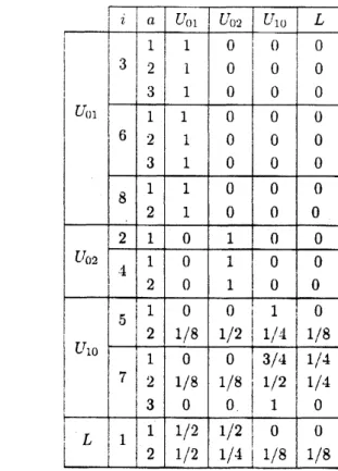
Let $\mathcal{K}=\{(.\mathrm{s}.j)|0\leqq s\leqq n^{*}, 1\leqq j\leqq l_{s}\}$ where $\eta^{*}$ and $l_{b}$ are given in Theorem 2.2. For $D\subset S.$ let $q_{i(}’D|a$) $:= \sum_{j\in D^{jij}}‘((x)$. In the ensuring discussion,

we

give the value

iteration algorithm, called Algorithm $\mathrm{C}^{-}$. with data in Table 1.

1. Set, $\gamma l\text{ノ}=1.g_{s_{I}}(1)=g_{b\dot{/}}^{\tau}$ for $(_{\mathrm{t}5_{i}}j)\in \mathcal{K}$ and $g_{i}(1)=\iota’\{d_{1}\}(i)$ for $i\in L$,

where $d_{1}(i, a)= \sum_{(\wedge^{-j)\in \mathcal{K}}}.q_{i}(U_{\forall j}|a).q_{b}j(1)$.

2. Suppose that $\{g_{sj}(n) : (s,j)\in \mathcal{K}\}$ and $\{g_{?}(n) : i\in L\}$

are

given $(n\geqq 1)$

.

Let for $i\in S-L$,

(4.2) _{$.q_{7}= \max_{a\in.4(i)}4\{d_{n}(i, a)+\sum_{j\in L}q_{ij}(a)g_{j}(n)\}$}

.

where $d_{n}(i.a)= \sum_{(s,j)\in \mathcal{K}}q_{j}(\mathrm{L}_{t\mathrm{j}}^{l}’,|\mathit{0}).q_{sj}(n)$

.

Let $g_{\epsilon j}(n+1)= \max_{i\in L^{r}}.g_{i}j$ and $g_{i}(n+1)=\iota’\{d_{n}\}(i)$ for $i\in L$

.

3. Let $n=\gamma’\neq 1$ and go to Step 2.

Concerning with Algorithm $\mathrm{C}^{-}$. we have the following.

Lemma 4.1 ([10]). In Algorithm $\mathrm{C}^{\tau}$

.

$u’e$ have:

(i) It holds that

(4.3) $g_{\epsilon j}(n+1)\geqq g_{sj}(n)$

for

$(s,j)\in \mathcal{K}$

.

and

(4.4) $.q_{i}(n_{\iota}+1)\geqq.q_{i}(\uparrow?)$

for

$i\in L$.

(ii) The Algorithm $\mathrm{C}^{\Gamma}$ converges. $i.e.$, when

$narrow\infty g_{sj}(n)arrow\overline{g}_{sj}$

for

$(s, j)\in \mathcal{K}$ and

$.q_{i}.(n)arrow\overline{.\mathrm{r}/}_{i}.\dagger\dot{\mathit{0}}ri\in L$.

For $\overline{.q}_{sj}$ and $\overline{.(J}$; in Lemnla 4.1. we have the following.

(4.5) _{$\overline{g}_{\hslash}J=\max_{a\in\swarrow \mathrm{i}(i)}\{d(i.a)+\sum_{j\in I_{J}}q_{ij}(a)\overline{g}_{j}\}$} for $i\in U_{sj}$ and $(s.j)\in \mathcal{K}$,

and

(4.6) $\overline{y}_{i}=\max_{a\in_{t}\mathrm{t}(ij}.\{d(i_{\iota}.a)+\sum_{j\in L}q_{i_{J}}(a)\overline{.q}_{j}\}$ for

$i\in L$,

where $d(i, a)= \sum_{(s.j)\in \mathcal{K}}q_{i}(U_{sj}|a)\overline{.}q_{sj}$.

Let $f^{*}$ be any stationarypolicy such that

$\backslash (4.7)$ f*(ノi) $=\{$

$f_{0j}(i)$ for $\prime i,$ $\in U_{0j}(1\leqq j\leqq l_{0})$

allv $\mathrm{m}\mathrm{a}\backslash \mathrm{i}\mathrm{m}\mathrm{i}\mathrm{z}\mathrm{e}\mathrm{r}$in (4.5) and (4.6) for _{$i\in S_{1}$}.

Since $\overline{.q}_{sj}.\overline{.q}_{t}$ and $f^{*}$ in $\iota^{4.5)-(4.7)}/$ are depending on $\tau\in(0,1)$, we denote them bv$\neg\neg g_{sj}.g_{i}$

and $f_{\wedge}^{*}$ respectively. Then,

we

have the following from Theorem

3.1.

Theorem 4.1. It holds that

(i) there exists $\tau_{0}\in(0.1)$ such that$f_{\tau}^{*}$ is average optimal

for

any $\tau(0<\tau<\tau_{0^{\backslash }},$, and

5

A numerical

example

Here, _inorderto$\mathrm{c}\cdot 0\iota \mathrm{n}\mathrm{p}\mathrm{r}e\mathrm{h}\mathrm{e}\mathrm{n}\mathrm{d}$

our

modified algorithlns workingeffectivelv wewill consider

a

llurnerical exarnple as follows, _{which is dealt} $\mathfrak{n}^{\gamma}\mathrm{i}\mathrm{t}1_{1}$ in [10]. In

our

previous

work[10], the finding of an optimal policy for edch conimunicating subset is supposedto us$e$ thepolicy

improvement. In this paper, we

use

the nearly optimal policy $\overline{f}_{\tau}$ and nearly optimal

average

reward $\neg g_{sj},$ $(.5, j)\in \mathcal{K}$ in each communicating sub-MMDPs with

sufficientlv

small

$\tau>0$

.

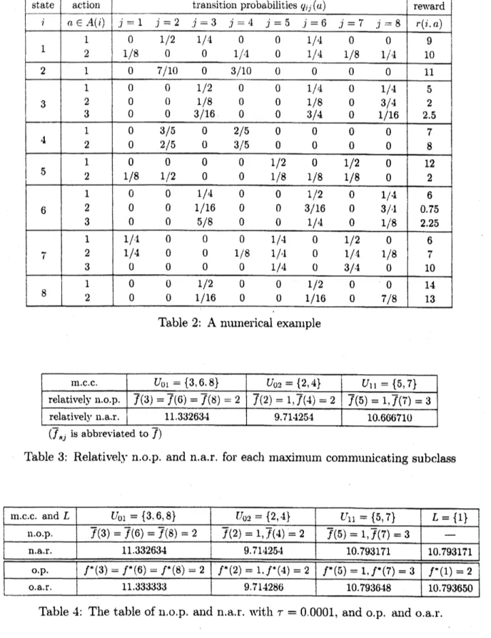
Let $S=\{1.2,3., 4.5,6,7.8\}$ and $A4(1)=\{1,2\},$$\lrcorner 4(2)=\{1\}\text{ノ}.A(3)=\{1,2,3\},$$A(4)=$ $\{1,2\}$,-4(5) $=\{1,2\}..4(6)=\{1.2,3\},$ $A(7)=\{1.2\}$ and $A(8)=\{1,2.3\}_{i}$ whose

transi-tion probability matrix $Q=(q_{ij}(\mathit{0}))$ and rewards $r=r(i, a),$$i.j\text{ノ}\in S.,$$a\in A(i)$

are

given

in Table 2.

First, applving the Algorithm A

we

have

the

$\mathfrak{c}\cdot‘ \mathrm{l}\mathrm{a}\mathrm{s}\mathrm{s}\mathrm{i}\mathrm{f}\mathrm{i}\mathrm{c}\mathrm{a}\mathrm{t}\mathrm{i}\mathrm{o}\mathrm{n}$ of the states: $S=U_{01}+U_{02}+L$

.

where $U_{01}=\{3,6.8\},$$U_{02}=\{2,4\},$ $L=\{1,5,7\}$. Next.

we

apply Algorithm $\mathrm{B}$ to the set of transient states $L=\{1,5,7\}$. Then, we find the maximum sub-MDP

$\Gamma_{1}=(S_{1}, \{-4_{1}(i), i\in S_{1}\}, Q_{S_{1}}. r_{S_{1}})$

where

_Si

$=\{5.7\}.\wedge 4_{1}(5)=\{1\},$$.4_{1}(_{l^{7}})=\{3\}$ and $Qs_{1},$$?s_{1}$

are

restrictions of Q.$\gamma$ on

$i,$$j\in S_{1}$ and $a\in.4(i_{1})$. $i_{1}\in S\mathrm{i},$ respectively. Applying Algorithm A to $\Gamma_{1}$, we find that $\Gamma_{1}$ is communicating and hence

we

set _{$L_{11}^{r}=\{5.7\}$}

.

In the end, the decomposition of $S$ in (2.7) is shown

as

$S=C_{01}^{\tau}+C_{02}^{T}+U_{11}^{\tau}+L$ with _$L=\{1\}$.

Next, _{for each communicating class}

_we

_{calculateanearly optimal polic.}$\mathrm{v}$($\mathrm{n}.0.\mathrm{p}.$, forshort)

and nearly optimal average $\mathrm{r}\mathrm{e}\backslash \backslash r\mathrm{a}\mathrm{r}\mathrm{d}$(n.a.r., for short) through

the vanishing discount ap-proach. We set discount rate $\tau=0.0001$ and $g_{sj}^{\tau}$. $(s, j)\in \mathcal{K}$ are replaced by arithmetic

mean of $\overline{l}\overline{\tau^{1}}_{r}(i)$

.

$i\in C^{T_{\epsilon^{\backslash }j}}$ where $’\overline{\prime\iota_{\text{ノ}\sim}’},$$(i)$ is

n.a.r.

by value iteration with repeating the steps

$n$ until $\mathrm{I}\mathrm{I}1\ \backslash _{i\in L_{sj}^{r}}|\overline{\mathrm{t}^{\prime^{\gamma\iota+1}}}_{\mathcal{T}}(i)-\overline{l^{1}}_{\mathcal{T}}(ni)|<\vee-:=10^{-6}$. Then, data in Table 1 is given in Table 3.

Applying Algorithm $\mathrm{C}^{\tau}$ to Table 3, we have n.o.p. and n.a.r. as in Table 4.

More-over.

if we use the policy iteration algorithm for each m.c.c. in order to get relatively

$\mathrm{a}.\mathrm{r}.$

.

then applying Algorithm $\mathrm{C}$ in _$[10]/\cdot$ the optimal policy(

$0.\mathrm{p}.$, forshort) and optimal

average rewards(o.a.p., for short)

can

be found

as

in Table 4 such that

$f^{*}(3)=f^{*}(6^{\backslash })=f^{*}(8)=2.f^{*}(2\grave{)}=1, f^{*}(4)=‘ 2.f^{*}(5)=1,$_{$f^{*}(7)=3.f^{*}(1)=2$}

and

$\psi’,’(*3)=\iota^{*}’(6)=\tau.\cdot(*8)=11.3^{\ell}3$3333;$\mathrm{t}^{j^{*}}’(2)=\mathrm{L}’)(;*4)=9.714286$.

4’“

(5) $=\iota^{*}’(7)\cong 10.793648,$$’^{*}(1)\cong 10.793650$.

It is noted that in Algorithm $\mathrm{C}^{\tau}$, the process

are

lulnped

as

Table 5. On the other

hand. by using the iterative method$(_{\lfloor}\mathrm{i}8])$ with the salne rule $\epsilon=10^{-6}$ for repeating the algorithm we have the following result as in Table 6 through Algorithm $\mathrm{C}$ in [10].

Whilc the algorithm in the iterative met,hod$([8])$ calculates nearly optimal

average

rcwards directly, the vanishing discount approach calculates nearly optimal

discount

reward $\mathrm{T}_{\tau}$ firstlv. and then $\mathrm{n}.\mathrm{a}.\mathrm{r}$. is given by $\tau\overline{\mathrm{t}’}-$. Hence, for sufficiently small

$\tau>$

{$)$.

$\tau^{r_{\dot{t}}}\iota \mathrm{r}\mathrm{l}\mathrm{i}\iota 9\mathrm{I}\mathrm{l}\mathrm{i}_{1\mathrm{l}}\mathrm{g}\mathrm{t}\mathrm{l}\mathrm{i}.\backslash ’ \mathrm{t}’\mathrm{O}1111\mathrm{t}\mathrm{a}\mathrm{p}\mathrm{p}\mathrm{r}${$)\mathrm{a}\mathrm{c}\cdot 1_{1}\mathrm{t}_{\dot{\zeta}}11$ get

$\mathrm{I}\mathrm{I}\mathrm{l}\mathrm{O}1^{\cdot}\mathrm{t}^{\backslash }$ significaiit digits which is close to the

optimal value than the method in [8] if

we

repeat the value iteration algorithm until

$\mathrm{n})\mathrm{a}_{\mathrm{R}\in L_{\mathrm{r}j}^{r}}|\overline{\prime n}_{\tau}^{n+1}(i)-\overline{v}_{\frac{n}{(}}(i)|<\epsilon$. Moreover,

our

modified algorithln onlv use value iteration

method,

_so

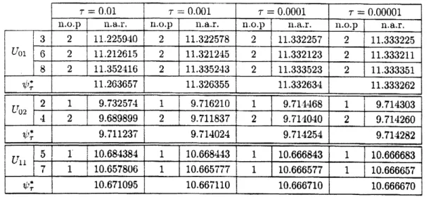
that it is easilyt,o_{calculatethenearly optinial valueswithsmaller numbers of}

multiplication per iteration than other algorithms. Table 7shows the results of applying the Algorithm $\mathrm{C}^{\overline{Z}}$ for

sorne cases

of

$\tau$. $\mathrm{T}_{\dot{C}}\iota\iota_{)}1\mathrm{t}^{\backslash J}.1$ illiistrates that our

$\mathrm{m}o$dified $\dot{r}1_{\lrcorner}1,\sigma,\mathrm{o}\mathrm{r}\mathrm{i}\mathrm{t}11\mathrm{I}\mathrm{I}1$

works well in this exainple.

References

[$1_{\mathrm{I},\lrcorner}^{1}$ John Bather. Optimal decision procedures for finite Markov chains. II.

Commluii-cating syst$e\ln_{\iota}\backslash ^{\backslash }$

.

Advances in Appl. Probability. 5:521-540,

1973.

[2] Richard Bellman. Dynamic progmmming. Princeton Univeristy Press, Princeton,

N. J., _1957.

[$3_{\mathrm{J}}^{\rceil}$ Eric V. Denardo. Contractionmappings in the theory underlying dynamic

prograln-ming. SIAMRev., 9:165-177, 1967.

[4] Eric V. Denardo. Dynamic programming: mod.els and applications.

_{Prentice-Hall:}

Inc., Englewood Cliffs. N. J., _1982.

[5] A. Federgruen and P. J. $\mathrm{S}\mathrm{c}\mathrm{h}\backslash \backslash r\mathrm{e}\mathrm{i}\mathrm{t}\mathrm{z}\mathrm{e}\mathrm{r}$

.

Discounted and

undiscounted

value-iteration

in

Markov

decision problems:

a

survey. In

Dynamic programming

and

its

applica-tions (Proc.

_Conf..

Univ. British Columbia, $\dagger/\acute{a}ncou\tau\dagger e’r_{:}B.C.,$ $\mathit{1}\mathit{9}77$),

pages 23-52.

Academic Press, New York, _1978.

[6] A. Hordijk and L. C. M. Kallenberg. Linear programming and Markov decision

chains. Management Sci., $25(4):352-362$

.

1979/80.

[7] Arie Hordijk and Martin L. Puterman.

On

the convergence of policy iteration in finitestate undiscounted Markov decisionprocesses: the unichain

case.

Math. Oper.

Res.. $12(1):163-176$, 1987.

[8] Arie Hordijk and Henk

_Ti.

$|\iota \mathrm{n}\mathrm{s}$. A modified form ofthe iterative method of dynamic

programming. .$4nn$

.

Statist..

3:203-208,

1975.

[9] Ronald A. Howard. Dynamic programming and $\Lambda Iar\cdot kov$processes. The Technology

Press ofM.I.T., Cambridge. Mass.. 1960.

[10] T. Iki, _{M. Horiguchi, aiid M. Kurano. A} struct,ured _{pattern lnatrix algorithnl for}

multichain $\mathrm{n}\mathrm{l}\mathrm{a}\mathrm{r}\mathrm{k}_{0\backslash }$, decision

processes.

(preprint). 2005.

[11] T. Iki. M. Horiguchi, M. Yasuda. and M. Kurano. Alearning algorithm for

commu-nicating markov decision processes with unknown transition matrices. (poeprint).

[12] John G. Kemeny arid J. Laurie Snell. Finite Markov chains. The UnivcrsitySeries in Undergraduate MMathematics. D. Van Nostrand Co., Inc.. Princeton,

N.J.-Toronto-London-New York, _1960.

[$13_{\mathrm{j}}^{\tau}$ Arie Leizarowitz. Analgorithm to identifv and compute average optimal policies in

multichain Markov decision processes. Math. Oper.

_Res.:

$28(3):553-586$, 2003.

[14] K. Ohno. A value iteration method for undiscounted multichain Markov decision processes. Z. Oper. Res., $32(2):71-93$, 1988.

[15] $\wedge\backslash \mathrm{I}\mathrm{a}\mathrm{l}\mathrm{t}\mathrm{i}\mathrm{n}$ L. Puterman. Mark

$ov$ decision processes: discrete stochastic dynamic

pro-gramming. John Wiley& Sons Inc., New York, 1994. A Wiley-Interscience

Publi-cation.

[16] P. .l. Schweitzer. Iterative solution of the functional equations of undiscounted Markov renewal programnuing. J. Math. Anal. Appl., 34:495-501, 1971.

[17] P. J. Schweitzer. A value-iteration scheme for imdiscounted multichain Markov renewal programs. Z. Oper. Res. Ser. A-B, $28(.5):\mathrm{A}143$ A152,

1984.

[18] E. Seneta. Nonnegattive $matr\dot{\mathrm{v}}ces$ and Markov chains. Springer Series in Statistics.

Springer-Verlag. New York, _second edition,

_1981.

[19] D. .l. XVhite. Dyuamic programming, $\mathrm{h}\prime \mathrm{f}\mathrm{a}\mathrm{r}\mathrm{k}\mathrm{o}\iota^{\gamma}$chains, and the methodofsuccessive

approximations. J. Math.

Anal.

Appl..

6:373-376.

1963.

$\perp \mathrm{a}\mathrm{o}\mathrm{l}\mathrm{e}$ -: $t1$ nulllerlcal exalllple

Table 3: Relatively n.o.p. and n.a.r. for each maximum $\mathrm{c}\mathrm{o}\mathrm{m}\mathrm{m}\mathrm{u}\mathrm{I}\dot{\mathrm{u}}\mathrm{c}\mathrm{a}\mathrm{t}\mathrm{i}\mathrm{n}\mathrm{g}$subclass

Table 5: Lumped transition matrix

Table

6:

The $t$able of n.o.p. and $\mathrm{n}.\mathrm{a}.1^{\cdot}$. with $\tau=0.0001$ by using the iterative nrethod in