A numerical study on the influence of non-axisymmetric flow perturbations on the hole-tone feedback cycle(Mathematical Aspects and Applications of Wave Phenomena)

A

numerical study

on

the influence of

non-axisymmetric flow

perturbations

on

the

hole-tone

feedback cycle

MIKAEL

A. LANGTHJEM, MASAMI

NAKANO

Department of

Mechanical

Systems Engineering,

Faculty of

Engineering,

Yamagata University,

Jonan

4-chomc,

Yonezawa-shi,

992-8510

Japan

Abstract

The paperis concerned with theholetone feedbackcycleproblem, also known

as

Rayleigh’s

bird-call. A methodology for analyzing the influence of non-axisymmetricperturbations of

the jet on the sound generation is described. In future experiments, these perturbations

will be applied at the jet nozzle via piezoelectric or electro-mechanical actuators, placed

circumferentially insidethe nozzle at itsexit. Themathematicalmodel, which is thesubject

of the proeent paper, is based on athree-dimensional vortex method. The nozzle and the

holedend-plate are representedby quadrilateral vortex panels, while the shear layer of the

jet is represented by vortexrings, composed ofvortex filaments. The sound generation is

described mathematically using the Powell-Howe theory ofvortex sound. The aim of the

work is to understand the effects ofa variety of flowperturbatioms, in order to control the

flowand theaccompanyingsound generation.

Keywords: aeroacoustics, self-sustained flow oscillations, three-dimensionalvortex method

1

Introduction

Self-sustained

fluid oscillations can

occur

in

a

variety ofpractical applicationswhere

a

shear

layer impinges upon

a

solid structure [1]. The oscillations

are

the

cause

of sound generation,

which typically is powerful. In

cases

of music instruments (flutes, etc.) and whistles, sound

generation is, of course, the aim. By engineeringapplications however, the sound generation is,

in most cases,

an

unwanted, annoying side effect.

The present paper is concerned with the so-called holetone problem $[2, 3]$

.

The

common

teapot whistle is an example ofutilization of the sound generation in this system. The steam

jet, issuing from

a

nozzle, passes through

a

similar hole in

a

plate, placed

a

little downstream from the nozzle.

The

shearlayerofthe jet is unstable and rolls up into

a

large, coherent vortex

(’anoke-ring’). This large vortex cannot pass through the hole in the plate and hits the edge

ofthe hole, where it creates

a

pressure

disturbance.

The disturbance is thrown back (with the

speed ofsound) to the nozzle, where it disturbs the shear layer. This initiatesthe roll-up ofa

new

coherent vortex. In this way an acoustic feedbadc loop is formed. Figure l(a) ilustrates

the principle of thehole-tonephenomenon. Figure l(b) shows

an

experimental realization, with

(a) (b)

Figure 1: (a) Geometry and physical features of the hole-tone problem. (b) Flow visualization

ofthe vortex roll-up [4].

The basic dynamics of the hole-tone feedback system

was

studied numericafy in Ref. [5],

using

an

axisymmetric vortex element method, combined with

an

aeroacoustic model based

on

Curle’s equation [6]. It

was

found that this methodology could predict the fundamental

iaracteristics

ofthe problem quite well, in particular the fluid-dynamic characteristics.

The bird-call,

as

described in Rayleigh’s The Theory

_of

Sound [2] is a small whistle for

simulating birdsong. It has been speculated at some point that the hole-tone phenomenon

may be the fundamental mechanism ofreal whistled birdsong, although the idea

seems

to be

abandoned at present [7]. The hole-tone system is however

a

partofmanyengineeringsystems,

wheresound generationisunwanted. Examplesinclude automobile intake-and exhaust systems,

$gas/steam$ _distribution systems (bellows, valves, etc.), and solid-propellant rocket motors. In

these cases, ifageometry which avoids the sound-generation cannot easilybeobtained,

a

control

method which

can

eliminate,or at least suppress, the sound generation is desirable.

Nakano et

at.

[4] studied experimentally

a

forced excitationstrategy to eliminate the hole

tone

feedback

cycle in

the

system depicted in Fig.

1.

The

shear

layer

near

the

nozzle

exit

was

excited acousticallyby

means

of

an

excitation chamber equipped with sixloudIpeakers, placed

equidistantly around the circumference. By hamonic, axisymmetric excitation at

&equencies

away $kom$ the fundamental frequency $f_{0}$, noise level reductions (at $f_{0}$) of up to 6 $dB$

were

achieved. A part of theseexperiments

were

simulated numerically in Ref. [8]. It

was

found that

forced acoustic excitation of the shear layer could suppress the sound pressure level, but to a

lesser degree than in the experiments.

The aim of the present work is to develop a simple and efficient numerical method for

a

full three-dimensional simulation of the hole-tone problem with the jet subjected to

non-$\dot{K}S\Psi^{nmet\dot{n}c}$‘mechanical’ (’non-acoustic’) perturbations,bypiezoelectric

or

electremechanical

actuators mounted around the circumference at the nozzle exit, similar to the experimental

concept of Kasagi [9]. With this concept,

a

variety ofexcitation modes and control laws

can

be

realized. Kasagi [9] praeents

some

very interesting experimental results related to

a

ffeejet. A

purpose of thepresentwork is to investigate how, andto what extent, variousexcitationmodes

(with vaiious degrees ofsymmetry) are able to suppress the noise generation in the hole-tone

problem.

Similar to

our

previous study [5], the present

one

is also based

on

a vortex method. Vortex

to shear layers constituting only a small part of the overall fluid volume [10]. It has recently

been shown [11] that numerical simulations with three-dimensional vortex filaments produce

characteristics of turbulent flows which agree well with experiments and direct numerical

simu-lations (based

on

theNavier-Stokesequations). The present work isbasedonthe vortex

_filament

method, similar to the work of Cortelezzi and Karagoizian [12], dealing with ajet in crossflow.

Altematively, the vortex partide method could have been chosen; this is done, for example, in

the work ofKiya et al. [13], dealing with forced excitation of

a

heejet.

The paper also includesadiscussion of the acoustic modelling, althoughno numerical results

are

presented. This includesan acousticfeedbackmodel, e.g. amodel of the back-reactionfrom

the acoustic fieldonto the freevortices. The soundpressure is computed usingthe vortexsound

model ofPowell [14] andHowe [15]. As in Lighthill’s original acoustic analogy [16], it is assumed

inthe vortex sound theory that there is

no

acoustic back-reaction from the acoustic field to the

sound-generating bankground flow. Yet it is thought to be plausible to include an acoustic

feedback $mo$del in connection with atimestepping simulation approach, as the present.

2

Flow

model

$(a)$ Modelling

of

the jet

The shear layer of the jet issuing from the nozzle is represented in a lumped form, by a

‘ne&laoe’ ofdiscretevortexrings. Theseringsare disturbedmechanically atthe nozzleexit such

that they loosetheir natural axisymmetric form, and

are

thusrepresented by three-dimensional

vortex filaments. The inducedvelocity $4=(u_{1}, u_{2}, u_{3})_{i}$, at position $x:=(x_{1}, x_{2}, x_{3})_{i}$ and time

$t$, from $J$ vortex rings represented bythe space

curves

_{$r_{j}(\xi,t),$ $j=1,2,$}

$\ldots$ ,$J$, isgiven by [17]

$u_{1}(x_{1},t)=-\sum_{j=1}^{J}\frac{\Gamma_{j}}{4\pi}\int_{\xi}\frac{[x_{1}(t)-r_{j}(\xi,t)]x\partial r_{j}/\partial\xi}{(|r(t)-r_{j}(\xi,t)|^{2}+\alpha\sigma_{j}^{2}(\xi,t))^{s}z}d\xi$, (1)

where$\Gamma_{j}$ isthe strength (circulation) ofthe$j’ th$vortex, $\xi$isamaterial (vortex) coordinate, and

$\sigma_{j}(\xi,t)$ is the

core

radius. $\alpha$ representsthe vorticity distribution within the

core.

An analytical

expression for this parameter

can

be derived [17]. For

a

Gaussian distribution, $\alpha\approx 0.413$

.

Thespace

curves

$r_{j}(\xi, t)$

are

discretizedby employing$K$marker pointsoneachcurve (vortex

ring), connected via cubic splines. These $spline8$ are expressed in the form of Ferguson

curve

segments(whichintum

are

based

on

Hermiteinterpolation). The integration is carried out using

Gauss-Legendre quadrature. [A simple linear interpolation

was

however employed to produce

the numerical examples in Section 4 of thepresentpaper.]

Avortexring isreleasedfromthe nozzle at each time stepinthe simulation. [Earlier studies

[5] have shown that the vortex shedding $hom$ _{the hole} in the end _{plate is insignificant.] The}

strength of the vortex ring to be released is dictated by the Kutta condition, which demands

that thepressure a little above the nozzle edge equalsthe pressure

a

little below.

The convection velocity of

a

shed vortex ring is dictated by the induced velocities from all other vortexrings, plustheself-inducedvelocity,

as

indicatedby (1). The positions$r_{i}$of the shed

vortex filament ring marker points

are

updated by solving numerically the system ofordinary

differential equations

$\frac{dr_{j}(t)}{dt}=4(r_{i},t)$, $i=1,2,$

$\ldots$ ,$Jx$ K. (2)

Except for the$vis\infty us$effectsimulated by theKuttacondition, thecomputations

are

basically

released. The volume of each individual ring must thus be kept constant; this constraint is

imposedvia the equations

$\frac{d}{dt}(\sigma_{j}^{2}\ell_{j})=0$, $j=1,2,$

$\ldots,$$J\cross K$, (3)

where $\ell_{j}$ is the instantaneous length of the $j$ th filament. There is however

one

exception to

this ‘principle’. Duringinteractionwithothervortexrings, stretching and folding into ‘hairpins’

may

occur.

When the fold angle is beyond

a

certainthreshold value,

a

hairpins is removedand the the ‘loose ends’ reconnected, in accordance with the idea proposed by Chorin [18]. Thereby

thevolume ofthe vortex ring is reduced. Thisimplies

a

reduction inthe energyof the ring, and

amounts to

a

simple dissipation mechanism.

$(b)$ Modelling

of

the solid

surfaces

The solid surfaces are repraeented by quadrilateral vortex panels, made up of four straight

vortexfilaments,

as

indicated by Fig. 2. The inviscidboundarycondition of

zero

normalvelocity

is imposed at control points in the center of these panels. The

mean

jet flow is provided by a

number ofpanels placed on the ‘back’ of the nozzle tube. The strengths of the bound vortex

panels

are

dictated by the boundary conditions and by the

mean

jet velocity.

The$me\bm{i}anical/piezoelectric$ actuator system issimulated by periodicaldeformationsofthe

nozzle end section,

as

illustrated by Fig. 3.

Figure 2: Distribution of bound vortex filament panels on the nozzle and the end plate. The

startup vortexofthefraejetisalso showninthe figure. [Inthetext the notation$x=(x_{1}, x_{2}, x_{3})$

is used, rather than the notation $(x, y, z)$ _shown in this and in the following figures.]

Figure3: Illustration of the perturbationmechanism (actuator model). [Forpurpose of

3

Aeroacoustic

model

$(a)$ The vortex sound approach

of

Powell and Howe

The concept of vortex sound, introduced by Powell [14] and developed further by Howe

[15], is probably the most efficient formulation in connection with a vortex element method

[19]. In Howe’s formulationthe sound emissionis, forlow Mach-number flows, described by the

inhomogeneous wave equation

$\frac{1}{c_{0}^{2}}\frac{\partial^{2}B}{\partial t^{2}}-\nabla^{2}B=\nabla\cdot L$, (4)

where $B(x, t)Is\cdot the$ stagnation enthalpy, and $L=wxu$ is the vortex force, with _the vorticity

$w$ given by $\nabla xu$

.

The relation between the enthalpy $B$ and the acoustic pressure $p$

can

be

expressed

as

[20]

$\frac{\partial p}{\partial t}=\rho_{0}(\frac{\partial B}{\partial t}+u\cdot\nabla B)=\rho_{0^{\frac{DB}{Dt}}}$

.

(5)

In the

far

field,

the

convective term disappears, giving

the

simplerelation $p(x,t)\approx\rho_{0}B(x,t)$

.

The solution to (4) is given by

$B( x,t)=-l\int_{y}\nabla_{y}G(x,y, t-\tau)\cdot Ldyd\tau$

.

(6)

Here $G(x,y, t-\tau)$ is

a

Green’s function which satisfies the boundary value problem

$\frac{1}{c_{0}^{2}}\frac{\partial^{2}G}{\partial\tau^{2}}-\nabla_{y}^{2}G=\delta(x-y)\delta(t-\tau)$, (7)

$G=0$ _for $t<\tau$, and $\frac{\partial G}{\partial n}=0$

on

_$S$

.

$S$symbolizes the surface of the end plate, and _{$n=(n_{1},n_{2},n_{3})$} its normal vector. Furthermore,

$x$is

an

observation point and$y$

a

source

point (i.e.,

a

point

on

a vortex ring). An approximate

solution to (7), correct to dipole orderwhen $S$ is acoustically compact, is givenby the so-called

$\infty mpact$

Green’s

function $[19, 20]$

$G(x,y, t- \tau)\approx\frac{\delta(t-\tau-|X-Y|/c_{0})}{4\pi|X-Y|}$, (8)

where$X=(X_{1}(x), X_{2}(x),$$X_{3}(x))$,with$X_{i}=x:-\varphi_{1}^{*}(x)$,and similarlyfor Y. The function$\varphi_{1}^{*}(x)$

is the velocity potential of the flow produced by moving the surface $S$ (the end plate) at unit

speed in the i-direction. In the present problem, only $\varphi_{3}^{*}$ will be

non-zero

if it is assumed that

the thickness of theendplate is vanishingly small. On $S$

,

it satisfies the relation $\partial\varphi_{3}^{*}/\partial x_{3}=n_{3}$

.

Based

on

the employed vortex panel representation of the solid surfaces, $\varphi_{3}^{*}$ is easilydetermined

numerically.

The final expression for the stagnation enthalpy $B$ takes the form

$B(x,t)=$ $\sum_{j=1}^{3}\frac{1}{4\pi}\int_{y}[(wxu)_{j}(y,t_{r})\frac{X_{j}-Y_{j}}{|X-Y|^{3}}\nabla Y_{j}d^{3}y]_{t_{r}}$ (9)

$\sum_{j=1}^{3}\frac{1}{4\pi c_{0}}\int_{y}[\frac{\partial}{\partial t}\{(wxu)_{j}(y,t_{r})\frac{X_{j}-Y_{j}}{|X-Y|^{2}}\nabla Y_{j}\}d^{3}y]_{t,}$

.

Thesquare braCketswith subscript$t_{r}$indicate evaluation at the retarded time$t_{r}=t-|x-y|/c_{0}$

.

over

all free vortex filament rings. The number of free vortices typically becomes very large.

For numerical efficiency, it isthus important that this summation iscarried out simultaneously

with that in (2).

The firstterm in (9) will dominatein the

near

field; thesecondterm in the far field. Inmost

aeroacoustic analyses the interest is only in the far field sound, and the first term is discarded. The

reason

for keeping it here is that the far field sound pressure is difficult to

measure

in the

experiments [4], due toreflections$hom$ the surroundings. [An anechoic chamber is not available

at present.] Hence only the near field pressure is measured, and has to be computed

as

well.

Another

reason

for keeping the

near

fleld term is that (9) is used also to evaluate the acoustic

feedback. Thisis the subject of the following section.

$(b)$ Acoustic

feedback

modd

For low Mach number flows it is known that the feedback mechanism works

hydrodynami-cally (i.e., instantaneously, without $acoustic/compressibility$effects),

as

thenozzle then lies only

a

fraction ofthe fundamental $a\infty ustic$ wavelength

away

$hom$ the endplate. In

our

earlier work

[5],based

on

Curle’sequation,it

was

foundhowever,that

an

acoustic feedbacksignal

(compraes-ibility $\infty rrection’$) reinforced the characteristic holetone hequency component and its higher

harmonics. It is thus found interestingto investigate the effect of acousticfeedback also in the

present vortex sound model, although it is understood that near field acoustic variables are

difficult to $\infty mpute$

.

Theacousticallyinducedflow, withvelocity$v(x,t)$,is assumed to be

a

potentialflow,

super-imposed

on

the vortical ‘background flow’ (with velocity $u(x,$$t)$). The acoustic pressure$p(x,t)$

and the acoustic (disturbance) velocity $v(x, t)$ is then relatedvia the expression

$\frac{\partial p}{\partial t}=-\nabla\cdot v$, (10)

or

via

a

potential function, $\Psi(x, t)$

,

as

$p=m \frac{\partial\Psi}{\partial t}$ $v=-\nabla\Psi$

.

(11)

Equations (5) and (11) give the relation

$v=-\int\nabla$Bdt $- \int\int\nabla(u\cdot\nabla B)d\overline{t}dt$

.

(12)

$\vee v\overline{v_{conv}}$

Onlythe first (non-convective) term$v^{*}(x, t)$ of(12) will beshownhere. Using (9), it is givenby

$v_{k}^{*}(x, t)$ $=- \sum_{j=1}^{3}\frac{1}{4\pi d}\int_{y}[\frac{\partial}{\partial t}\{(wxu)_{j}\frac{X_{j}-Y_{j}}{|X-Y|^{3}}\nabla Y_{j}\nabla X_{k}(X_{k}-Y_{k})\}d^{3}y]_{t_{r}}$ (13)

$+$ $\sum_{j=1}^{3}\frac{1}{4\pi c_{0}}\int_{y}[(\omega xu)_{j}\frac{X_{j}-Y_{j}}{|X-Y|^{4}}\nabla Y_{j}\nabla X_{k}(X_{k}-Y_{k})d^{3}y]_{t_{r}}$

$\sum_{j=1}^{3}\frac{1}{4\pi}\int_{-\infty}^{t}\int_{y}[(wxu)_{j}\frac{3(X_{j}-Y_{j})}{|X-Y|^{5}}\nabla Y_{j}X_{k}(X_{k}-Y_{k})d^{3}y]_{t_{r}}d\tau$

$\sum_{j=1}^{3}\frac{1}{4\pi q)}\int_{y}[(wxu)_{j}\frac{\nabla X_{k}\nabla Y_{k}}{|X-Y|^{2}}d^{3}y]_{t_{r}}+\sum_{j=1}^{3}\frac{1}{4\pi}\int_{-\infty}^{t}\int_{y}[(wxu)_{j}\frac{\nabla X_{k}\nabla Y_{k}}{|X-Y|^{3}}d^{3}y]_{t_{r}}d\tau$

.

These$a\infty uItic$velocitiesact

as

disturbancestothehydrodynamic velocity field, and

are

imposed

4

Numerical

examples

$(a)$ $Sta\hslash$-up jet

The calculations of the present paper

were

carried out for a setup with nozzle and end

plate hole diameter $d_{\iota)}$ equal to 50

mm.

The outer diameter of the end plate is

250

mm. The

gap length $L$ is

50

mm, e.g., equal to $d_{0}$

.

The

mean

velocity _{$u_{0}$} of the air-jet is 10 $m/s$

.

At 20 $\circ c$ this corresponds to

a

Reynolds number _{$Re=u_{0}d_{0}/\nu\approx 3.3x10^{4}$}

and a Mach

number $M=u_{0}/c_{0}\approx 0.03$, where the speedof sound _{$c_{0}=340m/s$} and the kinematicviscosity

$\nu=1.5x10^{-5}m^{2}/s$

.

The vortex rings

are

discretized into 24 control points in azimuthal direction $(K=24)$

.

Linear interpolation between the control points is used to produce the examples to follow; the

integrals (1) can then be evaluated analytically. The first order Euler method is employed for

the time-integration of(2). The time-step $\Delta t=0.025h/u_{0}$

.

Figure_{4 shows the side view of the impulsively started flow. A ‘bir& eye-view’ of the system,}

after

500

time-steps, is shown in Fig. 5.

1.$f$ $1$ $0s$ $0$ $\iota.\epsilon$ $- 1$ $- 1.2$ ₂₁

,

_{a 墨 ‘ $4S$ 5}

300

time-steps

400

time-steps 500 timesteps

$Fi_{1}re4$: Sideview of the jet afterimpulsive start-up. _{The nozzle exit isat the abscissaposition}

2.5; the end platewith hole at position

_3.5.

$(b)$

Influence of

$non-\dot{m}symmet\dot{n}c$ perturbations

Figure 6 illustrates the influence ofthe nozzle excitation shown in Fig.

3.

The excitation

amplitude is $r_{0}/20$; the frequency is 300 Hz. Part (a) of Fig. 6 shows a sequence of side view

‘snapshots’ for the non-perturbed jet, while part (b) is for the perturbed jet. The coherent

‘smokering’ which develops in part (a) is clearly destroyed by the perturbations in part (b).

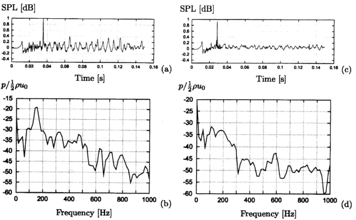
Figure 7 (a) shows the pressure on the end plate,

near

the edge of the hole. The signal

shown is the

mean

pressure, averaged

over

all control points at

one

particular radius, slightly

start-upvortexontothe endplate.] The correspondinghequency spectrumisshown in part (b).

Part (c) showsthe pressure signal for the perturbed flow, and part (d) the to (c) corresponding

frequencyspectrum.

As in part (a) of Fig. 7, part (c) shows the pressure averaged

over

the circumference. The

perturbations imply

that

negative and positive pressure contributions cancel out.

It

is then

not

surprisingthat the pressurepeaksdisappear.

From

a

hydrodynamic point ofview, the averaged

pressuresignalisnot really interesting. But$hom$

an

acoustic point ofview, the_{$intennediate/far$} fielddipolesoundcontribution isduetothe overallpressure fluctuations onthe plate. The result

givesthus

an

indicationthat non-axisymmetric perturbations may be effectivein cancelling the

flow-induced hole-tone sound.

Figure

5:

Birdseye-view ofthe system after

500

time-steps.

After 800 timesteps

900

time-steps

1000

time-steps

800

time-steps 900 time-steps

1000

time-steps

Figure6: Influenceof nozzleperturbations (asshowninFig. 3) ontheappearance of the jet. (a)

Unperturbed; (b) perturbed. A side view ofthejet is shown. The nozzle exit is at the abscissa

Figure 7: (a) Pressure fluctuations

near

the hole in the end plate. The signal shown is the

average of the pressure at allcontrol pointsat oneparticular radius, around the circumference.

(b) The to (a) corresponding ffequency spectrum. (c) Pressure fluctuations in the

case

of

a

perturbed jet (averaged signal,

as

in$(a)$). $(d)$ The to (c) corresponding spectrum.

5

Summary

In this paper a threedimensional vortex filament method, combined with an acoustic

feed-back model basedon thetheory of vortexsound, has been constructed. The purpose ofthework

is to study theinfluenceofnon-axisymmetric flowperturbations

on

the flowfield and thesound

generation in the holetone feedbaCk cycle problem. A few preliminary numerical studies have

been praeented. Comprehensive parameter studies

are

ongoing.

6

Acknowledgement

Thesupportof the present projectthrough

a JSPS

Grant-in-Aid forScientific Research (No.

18560152) is gratefully acknowledged.

References

[1] D. Rockwell, E. Naudascher, “Self-sustained oscillations of impinging free shear layers,”

Annu. Rev. Fluid Mech. 11, 67-94 (1979).

[2] Lord Rayleigh, The Theory

_of

Sound, Vol. II (Dover, New York, 1896, re-issued 1945).

[3] R.C.Chanaud, A. Powell, “Someexperimentsconcerningthehole and ringtone,” J.Acoust.

[4] M. Nakano, D. Tsuchidoi, K. Kohiyama, A. Rinoshika, K. Shirono, “Wavelet analysis

on

behavior of hole-tone self-sustained oscillation of impinging circular air jet subjected to

acoustic excitation,” (In Japanese) Kashikajouhou 24,

87-90

(2004).

[5] M. A. Langthjem, _{M. Nakano, “A numerical simulation of the holetone feedback} cycle

based on an axisymmetric discrete vortex method and Curle’s equation,” J. Sound and

Vibr. 288,

133-176

(2005).

[6] N. Curle, “The influence of solid boundaries upon aerodynamic sound,” Proc. Roy. Soc.

Lond. A 231,

505-514

(1955).

[7] G. J. L. Beckers, R. A. Suthers, C. $t$

.

Cate, “Pure-tone birdsong by

resonance

filtering of

harmonicovertones,” Proc. Nat. Acad. Sci. 100,

7372-7376

(2003).

[8] M.

A. Langthjem,

M. Nakano, “The jet

hole-tone

oscillation cycle subjected to acoustic

excitation: A numerical studybased

on

an

axisymmetric vortex method,” in Jets, Wakes

and Separated Flows (JSME), edited by T. Shakouchi, F. Durst, and K. Toyoda

,

pp.

745-750,

2005.

[9] N. Kasagi, “Towardsmartcontrolof turbulentjet mixingand combustion,” in Jets, Wakes

andSeparatedFlows (JSME), editedby T.Shakouchi, F. Durst, andK. Toyoda,pp. 45-53,

2005.

[10] G.-H. Cottet, P. D. Koumoutsakos, Vortex Methods: Theory and Practice, (Cambridge

University Press, Cambridge, 2000).

[11] P. S. Bernard, “Turbulent flow properties of large-scale vortex systems,” Proc. Nat. Acad.

Sci.

103,

10174-10179

(2006).

[12] L. Cortelezzi, A. R. Karagozian, “On the formation ofthe counter-rotating vortex pair in

transverse jets,” J. Fluid Mech. 446,

347-373

(2001).

[13] M. Kiya, Y.Ido, H.Akiyama, “Vortical structure inforcedunsteadycircularjet: Simulation

by$3D$vortex method,” in Vortex Flows and Rdated Numetical Methods II (ESAIM Proc.),

edited by Y. Gagnon, G.-H. Cottet, D. G. Dritschel, A. F. Ghoniem, and E. Meiburg, pp.

503-520, 1996.

[14] A. Powell, “Theory of vortex sound,” J. Acoust. Soc. Am. 36,

177-195

(1964).

[15] M.S. Howe, “Contributions to the$th\infty ry$ofaerodynamic sound, withapplicationsto

excess

jet noise and thetheory ofthe flute,” J. Fluid Mech. 71,

625-673

(1975).

[16] M.

J.

Lighthill, “On sound generated aerodynamically. I. General theory,” Proc. Roy. Soc.

Lond. A 211,

564-587

(1952).

[17] A. Leonard, “Computing three-dimensional incompressible flows with vortex elements,”

Annu. Rev. Fluid Mech. 17,

523-559

(1985).

[18] A. J. Chorin, “Hairpin removal invortex interactions II,” J. Comp. Phys. 107, 1-9 (1993).

[19] M.S. Howe, “Vorticity and the theory ofaerodynamicsound,” J. Engng. Math. 41,

367-400

(2001).