Chaotic Binary Sequences with
Their.Applications
to Communications
Tohru
KOHDA
and Akio
TSUNEDA
$\mathrm{D}\mathrm{e}..\mathrm{p}\mathrm{a}\mathrm{r}\mathrm{t}_{1}11\mathrm{e}\mathrm{n}\mathrm{t}$ of Computer Science and
$\mathrm{c}_{0111\mathrm{m}}11\mathrm{n}\mathrm{i}\mathrm{C}\mathrm{a}\mathrm{t}\mathrm{i}\mathrm{o}\mathrm{n}$ Engineering,
Kyushu University
Abstract: In spread specfrllm $\mathrm{s}\mathrm{y}\mathrm{s}\mathrm{t}\mathrm{e}\mathrm{l}\iota \mathrm{l}\mathrm{s}$ . a lot of$\mathrm{p}_{\mathrm{S}\mathrm{e}\mathrm{u}\mathrm{d}-}\mathrm{o}\mathrm{r}\mathrm{a}\mathrm{n}\mathrm{d}\mathrm{o}\ln$nulnbers with good
prop-erties are required as spreading sequences, most of which are generated by linear feedback
shift register (LFSR). In this paper, we propose chaotic binary sequences which are based
on chaos generated by one-dilnensional nonlinear ergodic $111\mathrm{a}\mathrm{p}_{\mathrm{S}}$, and evaluate their
perfor-nlance.S in spread spectrum systems. Furthermore, we propose an illlage $\mathrm{c}\mathrm{o}\mathrm{l}\mathrm{n}\mathrm{l}\mathrm{l}\mathrm{l}\iota \mathrm{l}\mathrm{n}\mathrm{i}\mathrm{C}\mathrm{a}\mathrm{t}\mathrm{i}\mathrm{o}\mathrm{n}$
$\mathrm{s}_{v}\mathrm{v}\mathrm{s}\mathrm{t}\mathrm{e}\mathrm{n}1$based on SS techniques which utilize characteristics of chaotic binary sequences.
1
Introduction
Spread spectrum techniques are due primarily to properties of spreading sequences (or
pseudonoise $(\mathrm{p}\uparrow \mathrm{q}\mathrm{A})$ sequences)[1]. Various classes of PN sequences have been proposed most
of which are generated by LFSR (linear feedback shift registers) stlch as the families
of the Gold sequences and of the Kasami sequences with low even-correlation values [1].
On the other hand. we proposed $\mathrm{s}\mathrm{i}\mathrm{n}\mathrm{l}\mathrm{p}\mathrm{l}\mathrm{e}$ methods to obtain binary sequences from chaotic
trajectories generated by nonlinear ergodic maps whose even and odd correlation functions
can be theoretically given. The elnpirical distributions of correlation values of chaotic bit
sequences are shown to tend to the Gaussian distribution.
In this paper. we investigate the $\mathrm{p}\mathrm{e}\mathrm{r}\mathrm{f}\mathrm{o}\Gamma 11\mathrm{l}\mathrm{a}\mathrm{n}\mathrm{c}\mathrm{e}$of chaotic binary sequences as spreading
sequences empirically and theoretically. Furthermore, we propose an $\mathrm{i}_{1}\mathrm{n}\mathrm{a}\mathrm{g}\mathrm{e}$ communication
$\mathrm{s}\mathrm{y}‘ \mathrm{s}$telll based on SS techniques which utilize characteristics of chaotic binary sequences.
2
CDMA
System Based
on Direct
Sequence Spread
Spectrum
In direct seqllence spread spectrum $(\mathrm{D}\mathrm{S}/\mathrm{S}\mathrm{S})$ systems, data sylnbols are directly multiplied
bv a pseudonoise $(\mathrm{P}\wedge \mathrm{N})$ code or a spreading code, which is independent of the data. Such
systelns are due primarily to properties ofspreading sequences(or PN sequences) [1]. For
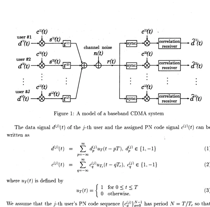
the most fundamental technique, both data symbols and code symbols are bipolar. Figure
1 shows a model of a CDMA $\mathrm{s}\mathrm{y}_{\mathrm{S}\mathrm{t}\mathrm{e}}\ln \mathrm{b}\mathrm{a}\mathrm{S}\mathrm{e}\mathrm{d}n$
on such $\mathrm{D}\mathrm{S}/\mathrm{S}\mathrm{S}$ techniques. For simplicity, we
consider baseband comnlunications. In such a $\mathrm{s}\mathrm{y}\mathrm{s}\mathrm{t}\mathrm{e}\mathrm{l}\mathrm{n}$, spread spectrulll signals of $J$ users,
$s^{(j)}(f),$ $j=1,2,$
Figure 1: A model ofa baseband CDMA system
The data signal $d^{(j)}(t)$ of the j-th user and the assigned PN code signal $c^{(j)}(t)$ can be
written as $d^{(j)}(t)$ $= \sum_{p=-\infty}^{\infty}d_{p}(j)u\tau(t-pT)$. $d_{p}^{(j)}\in\{1$.$-1\}$ (1) $c^{(j)}(t)$ $= \sum_{q=-\infty}^{\infty}Cu_{T_{c}}((qtj)-qT_{c}),$ $c_{q}^{(j)}\in\{1, -1\}$ (2) where $?l_{T}(t)$ is defined by $?l_{T}(\dagger)=\{$ 1 for $0\leq t\leq T$ $0$ otherwise. (3)
We $\mathrm{a}\mathrm{s}\mathrm{s}\mathrm{u}\ln e$ that the j-th
$\mathrm{u}.\mathrm{s}\mathrm{e}\mathrm{r}’ \mathrm{S}\mathrm{p}_{-}(j)(j)(j)\mathrm{v}\mathrm{c}\mathrm{o}\mathrm{d}\mathrm{e}$ sequence
$\{C^{(j)}\}pp=0^{1}\mathrm{A}--$ has period $N=T/T_{c}$ so that
there is a PN sequence $c_{0}$ ,$c_{1}.\cdots.c_{N-1}$ per data $\mathrm{s}\mathrm{y}\mathrm{n}\mathrm{l}\mathrm{b}_{\mathrm{o}1}$. For simplicity. assume that
$T_{r}=1$ through this paper. For a $\mathrm{D}\mathrm{S}/\mathrm{S}\mathrm{S}$ system, the PN code bit $c_{q}^{(j)}$ is referred to as a
chip. Thus the baseband spread spectrunl signal $S^{(j)}(t)$ is given by
$s^{(j)}(t\mathrm{I}=c^{(}j)(t)d(j)(t)$. (4)
For asynchronous $\mathrm{s}\mathrm{y}\mathrm{s}\mathrm{t}\mathrm{e}\mathrm{l}$)$\mathrm{l}\mathrm{s}$. the received signal $r(t)$ can be represented as
$r( \mathrm{t})=\sum_{j=1}^{J}c^{(}(t-t(j))j)d^{(j)}(t-\dagger)(j)+n(t)$ (5)
where $t^{(j)}$ is the $\mathrm{t}\mathrm{i}_{1}\mathrm{n}\mathrm{e}$ delay in thej-th channel and
$n(t)$ is a$\mathrm{c}\mathrm{o}\mathrm{n}\mathrm{l}\mathrm{m}\mathrm{o}\mathrm{n}$ channel noise process. If the received signal $r(t)$ is the input to the correlation $\mathrm{r}\mathrm{e}\mathrm{C}\mathrm{e}\mathrm{i}\mathrm{V}\mathrm{e}\mathrm{r}.\mathrm{m}\mathrm{a}\mathrm{t}_{\mathrm{C}\mathrm{h}\mathrm{e}\mathrm{d}}$to $S^{(i)}(t)$
.
theoutput during the p-th tinue-interval is
(8)
$\mathrm{A}\mathrm{s}\mathrm{s}\mathrm{U}\mathrm{n}\mathrm{l}\mathrm{e}$ that the system is quasi-synchronous (all of
$t^{(j)}$ are constrained to be integral
$111\mathrm{U}\mathrm{l}\mathrm{t}\mathrm{i}_{1})1\mathrm{e}\mathrm{s}$ of$T_{c}$) and $7?(t)=0$ and define $\ell_{ij}=\mathrm{f}^{(i)}-t^{(j}$). Then we can write
$Z_{\mathit{1})}^{()}i$ $=$ $N+I_{J,p}^{()}i$ (7)
$I_{J,p}^{(i)}$ $= \sum_{j=1}^{J}\{\frac{d_{p}^{(j)}+dp+1(j)}{2}.R^{E}(\ell ij;\{c^{()}\}i. \{c^{(}\}j))+\frac{d_{P}^{(j)}-dp+1(j)}{2}R^{o()}(\ell_{ij}; \{ci\}, \{_{C}(j)\})\}$
$j\neq i$
where $I_{J,p}^{(i)}$ denotes $\mathrm{c}\mathrm{o}$-channel interference from other $J-1$ channels and $R^{E}(P;\{c^{(i)}\}, \{C\}(j))$
and$R^{O}(l_{\backslash }.\{c^{(\uparrow)}\}, \{c^{(j)}\})$ denote theeven and the oddcross-correlationfilnctions,$\cdot$ respectively
$(0\leq[\leq\lrcorner\backslash ^{\tau}-1)$. Thev are defined by [1]
$R^{E}(l;\{c^{(}i)\}$. $\{C\}(j))=R^{A}(\ell,\cdot\{c\}(i). \{c)(j\})+R^{A}(N-\ell.;\{C(j)\}. \{c^{(i})\}\mathrm{I}$ (9)
$R^{o}(\zeta_{\backslash }.\{c\}(i), \{C\}(j))=RA(t_{\backslash }’\cdot\{C(i)\}.!\{C\}(j))-R^{4}(\mathit{1}\mathrm{V}-\ell’;\{c^{(j})\}$. $\{c^{(}.i)\})$ (10)
where $R^{A}(C_{\backslash }.\{c^{(i)}\}.\{c^{(j)}\})$ is called an aperiodic cross-correlation function or a partial
cor-relation filnction. defined by [1]
$R^{A}(C’; \{c\}(i), \{c)(j\})=\sum_{0\eta=}^{N}-1-lc_{n}^{(}c_{n+\ell}i)(j)$. (11)
In order to reduce $\mathrm{c}\mathrm{o}$-channel interference. absolute
$\mathrm{v}\mathrm{a}\mathrm{l}\iota \mathrm{l}\mathrm{e}\mathrm{S}$ of such even and odd
cross-correlation fiunctions. which depend on the $\mathrm{f}\mathrm{a}\mathrm{l}\mathrm{l}\mathrm{l}\mathrm{i}\mathrm{l}\mathrm{y}$ of PN sequences, are desired to be small.
3
Chaotic Bit Sequences
3.1
Generation
To give $\mathrm{n}1\mathrm{e}\mathrm{t}\mathrm{h}_{0}\mathrm{d}_{\mathrm{S}}$ for generating chaotic bit sequences., we
$\mathrm{d}\mathrm{i}\mathrm{s}\mathrm{c}\iota \mathrm{l}\mathrm{s}\mathrm{s}$the solutions of the
dif-ference $\mathrm{e}\mathrm{q}_{11\mathrm{a}}\mathrm{t}\mathrm{i}\mathrm{o}\mathrm{n}[2],[3]$
$\omega_{n+1}=’,$$(x_{n}),$ $\omega_{7?}\in I=[d, e]$. $n=0.1,2$.$\cdots$ (12)
where $\tau$ is a piecewise continuous function which lllapssome interval
$I$ into itself. It is well
known that the sollltions of $\mathrm{e}\mathrm{q}.(12)$ may be chaotic. For exalnple, the Chebyshev map of
degree $k$ with $I=[-1.1]$ defined by [4]
$\tau(\omega)=\cos(k\cos-1\omega),$ $k=2.3.4$. $\cdots$ (13)
have chaotic trajectories. In our previous study [5]., we proposed two simple methods to
obtain binary sequences fronl chaotic real-valued sequences $\{\tau^{n}(\omega)\}_{n=^{0}}\infty$. both of which can
give efficient methods to generate simultaneously different sequences ofi.i.d. binaryrandonl
Method-l: Using the threshold function defined by
$\ominus_{t}(\omega)=\{$
$0$ for $\omega<t$
(14) 1 for $\omega\geq t$,
we can obtain a binary sequence $\{\ominus_{t}(\omega_{n})\}_{n=0}^{\infty}$, which is referred to as a chaotic threshold
seqnence
(called a Chebyshev threshold $seq_{\mathrm{I}le}nce$ when $\tau(\cdot)$ is a Chebyshev polynomial).The second method was based on a binary expansion of the absolute value of $\omega$ when
$|_{A}‘)|\leq 1$ as follows.
Method-2: We write the value of$\omega(|\omega|\leq 1)$ in a binary representation:
$|\omega|=0.A_{1(\omega})A_{2}(\omega)\cdots A_{i(\omega})\cdots$ , $A_{i}(\omega)\in\{0,1\}$, $|\omega|\leq 1$. (15)
The i-th bit $A_{i}(\omega)$ can be expressed as
$A_{i}( \omega)=2i-1\sum_{r=1}(-1)r-1\{1-\ominus-\frac{\gamma}{\circ l,\sim}(\omega)+\frac{\mathrm{r}}{9^{l},\sim}(\omega)\}$ . (16)
Thus we can obtain a binarysequence $\{A_{i}(\omega_{n})\}^{\infty}n=0$ which we call a chaotic bit sequence (or
a Chebyshev bit sequencewhen $\tau(\cdot)$ is a Chebyshev polynomial).
3.2
Correlation
Properties
For any $L_{1}$ function $F(\cdot)$, consider the sunu defined by
$F_{l}.( \omega)=\frac{1}{N}\sum F(\mathcal{T}^{n}(\omega \mathit{1}n=0\mathrm{v}-1\mathrm{I}).$ $(1^{-}7)$
According to the Birchoff individual ergodic theorem [3]., we have
$Narrow\infty 1\mathrm{i}_{111}F_{N(\omega})=\langle F\rangle$ $\mathrm{a}.\mathrm{e}$. (18) under the $\mathrm{a}\mathrm{S}\mathrm{S}\mathrm{U}\mathrm{n}\mathrm{l}\mathrm{P}^{\mathrm{t}\mathrm{i}_{\mathrm{o}\mathrm{n}}}$ that $\tau(\cdot)$ is mixing on $I$ with respect to an absolutely continuous
invariant (or briefly ACI) nleas\iota lre, denoted by $f^{*}(\omega)d\omega$, where $\langle F\rangle$ is the enselllble-average
of$F$ over $I$, defined by
$\langle F\rangle=\int_{I}F(\omega)f^{*}(\omega)d\omega$. (19)
It is known that the enselllble average technique is useful in theoretically evaluating
statis-tics of chaotic sequences, such as lneans and correlation functions. Applying this technique
to several ergodic $\mathrm{n}\mathrm{u}\mathrm{a}_{\mathrm{P}^{\mathrm{S}}}$,
we
can getthe
fact that the chaotic binary sequences have goodNow weconsider two $\{0,1\}$-valued sequences $\{g(\tau^{n}(\omega))\}_{n=}\infty 0$ and $\{h(\tau^{n}(\omega))\}_{n=}\infty 0$. Define
$R_{N}( \omega.\ell;g.h)--\frac{1}{N}Nn=0\sum^{-1}(2g(\tau(n\omega))-1)(2h(\tau^{n}(+l)\omega)-1)$ (20)
which is the cross-correlation function between these two sequences $\mathrm{f}\mathrm{r}\mathrm{o}\ln$a seed
$\omega$, where $\ell$
is the $\mathrm{t}\mathrm{i}_{1}\mathrm{n}\mathrm{e}$ delay.
Let $X$ be a set of seeds and let $M$ be its cardinality. We introduce the average values
of$R_{\mathrm{V}}.(_{\iota I}.’\cdot g\ell_{\backslash }.h)$ over $\wedge Wf$ seeds given by
$\hat{R}_{\mathrm{A}}\mathrm{v},M(C;g, h)=\frac{1}{\mathit{1}\iota,f}\omega\in X\sum_{0m}RN(\omega 0m\cdot\ell;g.h)$. (21)
Then this function$\hat{R}_{\mathrm{A}}\mathrm{V}_{\angle,\vee}.’\mathrm{V}l.(\ell\backslash g, h).$
cal..l.ed
an empirical one, approaches to $\langle R(P;g, h)\rangle$ when $N$and $M$ are $\mathrm{s}\mathrm{u}\mathrm{f}\mathrm{f}\mathrm{i}\mathrm{c}\mathrm{i}\mathrm{e}\overline{\mathrm{n}}\mathrm{t}\overline{\mathrm{l}}\mathrm{y}$ large because
$\langle R(t;g.h)\rangle$ is regarded as the average over all possible
seeds.
.. Next. let $R_{\mathrm{V}\mathrm{A}}^{A}(\omega.\ell\backslash g.h)$ be an aperiodic correlation fllnction between two binary
se-quences $\{g(\tau^{n}(\omega))\}_{\eta=0^{1}}^{N-}$ and $\{h(\tau^{n}(d))\}_{n=0^{1}}^{\backslash }\gamma-$ defined as [1]
$R_{\perp \mathrm{V}} \wedge 4(\omega.C\text{ノ};g, h)=\frac{1}{\mathit{1}\backslash ^{\tau}}\sum^{N}(2g(\mathcal{T}^{n}(\omega \mathrm{I})-1)(2h(\mathcal{T}^{n+}\ell n=0(-1-l\omega))-1)$ (22)
which gives the even and odd correlation function to be considered in evaluating the
per-forlllance ofSS systems. Its $\mathrm{e}\mathrm{n}\mathrm{l}\mathrm{p}\mathrm{i}\mathrm{r}\mathrm{i}_{\mathrm{C}\mathrm{a}}1$ correlation function is given by
$\hat{R}_{\mathrm{V}\mathrm{A}M}^{A},(\ell\backslash g_{;}h)=(1-,\frac{\ell}{\wedge \mathrm{V}}\mathrm{I}\hat{R}N-l,M(\ell;g.\prime h).$ (23)
The $\mathrm{e}\mathrm{n}\mathrm{l}\mathrm{p}\mathrm{i}\mathrm{r}\mathrm{i}_{\mathrm{C}}\mathrm{a}1$ function $\hat{R}_{N-l,M(;}\ell g.h$) also $\mathrm{a}\mathrm{p}\mathrm{p}\mathrm{r}\mathrm{o}\mathrm{a}\mathrm{c}_{\lrcorner}\mathrm{h}\mathrm{e}\mathrm{S}$ to $\langle R(C;g, h)\rangle$ when $N$ and $M$ are
sufficiently large. Thus the enselnble average $\langle R_{\mathit{1}\mathrm{v}(;}^{A}\ell g, h)\rangle$ can be written as
$\langle R_{N}^{4}(c’\cdot g\backslash ’ h)\rangle=(1-\frac{p}{N})\langle R(\ell;g, h)\rangle$. (24)
Therefore. the theoreticaleven correlation function $\langle R_{N}^{E}(\ell;g.\prime h)\rangle$ and odd correlation
func-tion $\langle R_{N}^{O}(\ell’;g, h)\rangle$ are respectively given by
$\langle R_{N}^{E}(\ell;g.h)\rangle$ $=$ $\langle R_{N}^{A}(\ell;g, h)\rangle+\langle R_{N}^{A}(N-\ell;h, g)\rangle$, (25)
$\langle R_{\mathrm{V}}^{O}.(p;g, h)\rangle$ $=$ $\langle R_{N}^{A}(\ell;g, h)\rangle-\langle R_{N}^{A}(N-\ell;h.g)\rangle$. (26)
3.3
Numerical
Examples
Somenumerical examples ofeven and odd correlation functions of Chebyshev bit sequences
are shown. Figures 2 and 3 show the theoretical even (respectively odd) correlation
func-tions $\langle R_{N}^{E}(p;A_{i}.Aj)\rangle$ (respectively $\langle R_{\mathrm{V}}^{O}.(\ell;Ai,$ $Aj)\rangle$)
$’$
. indicated by solid lines, and the
$N=127$ and $M=100$. In each figure, the degree of Chebyshev maps and the bit
num-bers are indicated. The theoretical values are in good agreement with the $\mathrm{e}\ln_{\mathrm{P}^{\mathrm{i}\mathrm{r}\mathrm{i}\mathrm{c}\mathrm{a}1}}$
ones.
Besides. we can find that their cross-correlation values become low when the degree $k$ and
the bit numbers are large. Note that their auto-correlation values except $\ell=0$ are similar
to their cross-correlation values.
(a) even (b) odd
Figllre 2: (a) ($R_{N}^{E}(c;A_{2,}.A_{3})\rangle$ and$\hat{R}_{N,M}^{E}(\ell;A_{-},.A3),$ $(\mathrm{b})\langle R_{N}^{O}(\ell:A_{2}.,$$A3)\rangle$ and $\hat{R}_{N}^{o_{\mathrm{w}(p}},.;A_{2},$$A_{3}$)
where $\wedge \mathrm{V}=127.M’=100$, and $k=2$.
(a) even (b) odd
Figure 3: (a) $\langle R_{N}^{E}(\ell;A8, A9)\rangle$ and $\hat{R}_{\mathit{1}}^{E}\mathrm{V},M(\ell;A8\cdot A9).!(\mathrm{b})\langle R_{N}^{O}(\ell;A8, A9)\rangle$ and $\hat{R}_{\mathrm{V}}^{o_{M(\cdot A_{9}}}.,,\ell_{!}A_{8},$)
4Distributions of
Statistics
of
Chaotic Sequences
It should be noted that $R_{\mathit{1}\backslash ^{}(\omega}^{E},$$c^{};A_{i,j}A$) and $R_{l\backslash (}^{o_{\tau}}\omega,$$\ell;A_{i},$$A_{j}$) have large scattered values
because they are randonl variables. Thus we lnust investigate distributions of such randonl
variables for acertain set of seeds $\{\omega 0_{m}\}_{m=1}^{M}$ becausebit error probabilities in asynchronous
$\mathrm{C}\mathrm{D}_{\sim}\backslash \mathrm{I}\mathrm{A}\mathrm{s}\mathrm{y}_{\mathrm{S}}\mathrm{t}\mathrm{e}\mathrm{n}1.\mathrm{s}$ depend on distributions of correlation values. called
empirical
distributions.Figure 4 shows such empirical distributions of $\{R_{N}^{E}(\omega_{0m}.p_{:^{A_{i,j}}}.A)\}^{M}m=1$ and the ones of
$\{R_{\mathrm{v}}^{o_{(;A_{i}},\iota}.\omega 0_{m}\cdot\ell Aj)\}^{\angle}m=1l$
.
where $M=$ 8001. We can observe that these $\mathrm{d}\mathrm{i}\mathrm{s}\mathrm{t}\mathrm{r}\mathrm{i}\mathrm{b}_{1}1\mathrm{t}\mathrm{i}\mathrm{o}\mathrm{n}\mathrm{S}$tend to Gaussian distributions [6] defined $\mathrm{b}_{\vee}\mathrm{v}$$O( \omega)=\frac{1}{\sqrt{2\pi\sigma^{2}}}\exp[-\frac{(\omega-\nu)^{2}}{2\sigma^{2}}]$ , $(-\infty<\omega<\infty)$ (27)
where $\nu$ is lllean and
$\sigma^{2}$ is variance. Of course, the theoretical estinlates of
lnean, denoted
respectively by $\nu_{\tau}^{E}$ and $\nu_{\tau;}^{O}$ are respectively given by
$\nu_{\tau}^{E}$ $=$ $\langle R_{\mathrm{A}}^{E}4’(^{\ell};Ai, Aj)\rangle$, (28)
$\nu_{\tau}^{O}$ $=$ $\langle R_{\mathrm{V}}^{O}.(\ell;Ai, Aj)\rangle$ (29)
and those ofvariance. respectively denoted by $(\sigma_{\mathcal{T}}^{E})^{2}$ and $(\sigma_{\tau}^{O})^{2}$, are also given by
$(\sigma_{\mathcal{T}}^{E})^{2}-\sim$ $=$ $\langle(R_{\mathit{1}\mathrm{V}(\omega.\ell^{\mathfrak{d}};}^{E}Ai.\prime Aj))^{2}\rangle-\langle R_{N}^{E}(\omega, \ell;A_{i}, A_{j})\rangle.2$ (30)
$(\sigma_{\tau}^{O})^{2}---\langle(R_{f\backslash ^{r}(}^{O}.\omega.\ell;Ai\cdot Aj))2\rangle-\langle R_{N}o_{(i,j}A)\rangle 2\omega.\ell;A$. (31)
NVe refer to $\mathrm{t}\mathrm{h}\mathrm{e}\lambda$
Gaussian distribution with nlean $\nu_{\tau}^{E}$ (respectively $\nu_{\tau}^{O}$) and variance $(\sigma_{\tau}^{E})^{2}$
$(\mathrm{r}\mathrm{e}\mathrm{s}_{\mathrm{I}^{)}}\mathrm{e}\mathrm{C}\mathrm{t}\mathrm{i}_{\mathrm{V}\mathrm{e}}1_{\}^{\vee}}(\sigma_{\mathcal{T}}^{E})^{2})$ as the estimated distribution of $\{R_{\mathrm{A}}^{E}\mathrm{V}(\omega 0m’\zeta;A_{i}, A_{j})\}_{m1}^{\mathrm{t}t}\mathit{1}=$ (respectively $\{R_{N}^{o_{(;A_{i}}.\mathrm{A}}.\omega_{0}.c7\eta Aj)\}_{m1}^{\psi I}=)$. Figure 4 leads us to find that the theoretical estilluates of lllean
and variance are given by
$\nu_{\tau}^{E}$ $\simeq$ $0$ (32)
$\nu_{\tau}^{O}$ $\simeq$ $0$ (33)
$(\sigma_{\mathcal{T}}^{E})^{2}$ $\simeq$ $\frac{1}{N}$ (34)
$(\sigma_{\mathcal{T}}^{O2})$ $\simeq$ $\frac{1}{N}$ (35)
each of which is independent of the bit nunlbers $\dot{i},$ $j$ and the delay $\ell$ when the degree of
the Chebyshev map and the bit nunlbers are large. It is easily checked that the estimated
$\mathrm{d}\dot{\iota}\mathrm{s}\mathrm{f}\mathrm{r}\mathrm{i}\mathrm{b}\mathrm{l}\mathrm{l}\mathrm{t}\mathrm{i}\mathrm{o}\mathrm{n}$are in good
$\mathrm{a}\mathrm{g}_{\Gamma \mathrm{e}\mathrm{e}\mathrm{n}1}\mathrm{e}\mathrm{n}\mathrm{t}$with the empirical ones.
For colnparison, the distributions of correlation values ofGold sequences are shoxvn in
(a) even (b) odd
$\mathrm{F}\mathrm{i}\mathrm{g}_{11\mathrm{r}\mathrm{e}}4$: Distributions of correlation values of Chebyshev bit
$\mathrm{s}\mathrm{e}\mathrm{q}_{11}\mathrm{e}\mathrm{n}\mathrm{c}\mathrm{e}\mathrm{s}$, where $N=127.!$
$\wedge 1\prime I=8\mathrm{o}\mathrm{o}1,$ $(i,j)=(8,9)$, and $k=16$.
(a) evell (b) odd
$\mathrm{F}\mathrm{i}\mathrm{g}_{11}\mathrm{r}\mathrm{e}5:\mathrm{D}\mathrm{i}_{\mathrm{S}\mathrm{t}\mathrm{r}}\mathrm{i}\mathrm{b}_{1\iota}\mathrm{t}\mathrm{i}\mathrm{o}\mathrm{n}\mathrm{S}$of correlationvalllesof8001 pairs of Goldse(
$1^{11\mathrm{e}}\mathrm{n}\mathrm{c}\mathrm{e}\mathrm{S}$, where $N=127$.
5
Evaluation of
Bit
Error Probabilities
As is well known, bit error $1$)
$\mathrm{r}\mathrm{o}l$)$\mathrm{a}\mathrm{b}\mathrm{i}\mathrm{l}\mathrm{i}\mathrm{t}\mathrm{i}\mathrm{e}\mathrm{S}$ in asynchronolls
CDMA systems depelld on distri-butions ofeven and odd correlation vallles between each pair of$\mathrm{s}_{\mathrm{I}^{)\mathrm{r}\mathrm{e}\mathrm{a}\mathrm{d}\mathrm{i}}}\mathrm{n}\mathrm{g}\mathrm{S}\mathrm{e}(11\mathrm{l}\mathrm{e}\mathrm{n}\mathrm{c}\mathrm{e}‘ \mathrm{S}$.
.N$o\mathrm{w}$ assume that $J$ users communicate $\mathrm{t}\mathrm{h}_{\Gamma \mathrm{O}11}\mathrm{g}\mathrm{h}$ a CDMA system $\mathrm{i}\mathrm{n}\mathrm{d}\mathrm{e}_{1}$)$\mathrm{e}11\mathrm{d}\mathrm{e}\mathrm{n}\mathrm{t}1.\mathrm{v}$ and $\mathrm{c}_{1\mathrm{y}1}11\mathrm{a}\mathrm{s}\mathrm{i}-\mathrm{s}\mathrm{n}\mathrm{c}\mathrm{h}_{1}\cdot \mathrm{o}\mathrm{n}\mathrm{o}\iota 1\mathrm{S}\mathrm{y}.$ Thtls the distriblltion of the $\mathrm{c}\mathrm{o}$-channel interference to the i-th user from other $.J-1$ channels are $\mathrm{e}\mathrm{s}\mathrm{t}\mathrm{i}_{111}\mathrm{a}\mathrm{t}\mathrm{e}\mathrm{d}$ by the Gatlssian $\mathrm{d}\mathrm{i}\mathrm{S}\mathrm{t}\mathrm{r}\mathrm{i}\mathrm{b}_{1\iota}\mathrm{t}\mathrm{i}\mathrm{o}\mathrm{n}$ with mean $0$ and
variance $(J-1)N$ because of the additive property of the Gaussian distribution.
Fig-ure $6(\mathrm{a})$ shows numerical $\mathrm{e}\mathrm{x}\mathrm{a}\mathrm{m}_{\mathrm{I}^{1\mathrm{e}\mathrm{S}}}$) of $\mathrm{s}\iota \mathrm{l}\mathrm{c}\mathrm{h}$
distributions of the $\mathrm{c}o$-channel interference in $\mathrm{a}\mathrm{s}\mathrm{y}\mathrm{n}\mathrm{c}1_{1}\mathrm{r}\mathrm{o}\mathfrak{U}0\iota 1\mathrm{S}$ CDMA systems using Chebyshev bit
$\mathrm{s}\mathrm{e}\mathrm{q}\iota \mathrm{l}\mathrm{e}\mathrm{n}\mathrm{c}\mathrm{e}\mathrm{S}$. For reference. Figure $6(\mathrm{b})$
Chebyshev bit sequences tend to the Gaussian distribution irrespective of the number of
channels. On the otherhand, the onesfor Goldsequences are not the Gaussian distribution
when the number ofchannels, $J$, is small. However, it is shown that the distributions for
Gold sequences tend to the Gaussian distribution as the number of channels increases.
0.1 $0\uparrow 0$ $\mathrm{o}\underline’$ $N^{-}B\mathit{2}$ $[]$ $J=\mathit{3}\circ$ 64.487 $009$ $\circ$ , $\theta$ $J_{--}\mathit{4}*$ 95.880 ’ $J_{--}\mathit{5}\circ$ 127.728 $008$ $\mathrm{r}^{*}‘ \mathrm{r}$ 1 $0$
.
$\mathfrak{o}*_{\theta}$ 0.07 $\mathrm{o}^{*}\mathrm{o}$ $\mathrm{f}\mathrm{i}\mathrm{o}\mathrm{q})$ $*\circ$ ’ $0^{*}$ $0\circ$ $0_{0}$ $\approx\xi 0)0.\infty$ $*$ $*$ ’ $\mathrm{o}0.05$ $\circ\circ$ $\mathfrak{g}\circ$ $\mathrm{c}$ $\circ l$ $004$ $\circ*$ $\circ*$ $0_{9^{\mathrm{i}}}*$ $\mathrm{t}$ $0^{\circ}$0.03
.
$\square$ $\mathfrak{o}$ $\mathrm{O}^{*^{9}}$ $,.\circ$ 0.02 $0$ $\mathrm{O}^{*}$ ‘ $.\mathrm{e}_{\mathrm{O}}$ 001 $\circ\star$, $0^{\mathrm{g}\circ}$ $0_{*}^{\mathrm{o}_{*\mathrm{I}\circ}^{\mathrm{O}}}$ $c$ $c$ $\circ;^{\mathrm{O}}\^{\mathrm{o}_{\mathrm{O}}}$.
$c$ $0$ $- 40$ $- 20$ $0$ 20 40 interference(a) Chebvshev bit sequences (b) Gold sequences $arrow$
$\mathrm{F}\mathrm{i}\mathrm{g}_{11\mathrm{r}}\mathrm{e}6$: Distributions of $\mathrm{c}\mathrm{o}$-channel interference frolll $J-1$ channels in an asynchronous
CDMA system, where $N=32$.
The bit errors occllr when the $\mathrm{c}\mathrm{o}$-channel interference is greater than $N$ if the i-th
infomation bit during the p-th tinle-interval is $d_{p}^{(i)}=-1$ (or is snlaller $\mathrm{t}\mathrm{h}\mathrm{a}\mathrm{n}-\mathrm{j}^{\tau}$if the i-th
$\inf_{\mathrm{o}\mathrm{r}111}\mathrm{a}\mathrm{t}\mathrm{i}\mathrm{o}\mathrm{n}$ bit is $d_{p}^{(i)}\neg-1$). Hence, if $\mathrm{P}\mathrm{r}\{d_{p}^{(j})=1\}=\mathrm{P}\mathrm{r}\{d_{p}(j)=-1\}=\underline{‘\frac{1}{)}}$ for all $j$ and
$n(t)=0$, the bit
err\^Or
$\mathrm{p}\mathrm{r}\mathrm{o}..\mathrm{b}$ab..ility
can be estimated by $\simeq$ $\overline,.$: $P_{e}$ – $\mathrm{P}\mathrm{r}\{I_{J,p}^{(}i)>N|d_{p}(i)=-1\}$ (36)
$=$ $\int_{N}^{\infty}\frac{1}{\sqrt{2\pi\sigma-}},\exp[-\frac{\omega^{2}}{2\sigma^{2}}$. $]d\omega$ (37)
$=$ $Q( \frac{N}{\sigma})$ (38)
where
..,:.:
$l–\backslash \backslash \sim\backslash \cdot\backslash \triangleleft’..$. .:. , .$\cdot$ $..\cdot\cdot.-..$ . $\vee^{-}\cdot$ $\sigma^{-}$ ’ $=$ $(J-1)N$ (39) $Q(x)$ $=$ $\int_{x}^{\infty}\frac{1}{\sqrt{2\pi}}\exp[-\frac{\omega^{2}}{2}]d\omega$. (40)
The above quantity $P_{e}$ indicates that $N$ and $\sigma^{2}$ correspond respectively to $\sqrt{E_{b}}$and $-\mathrm{V}_{J}/2$
in the well-known bit
error
probability of a coherent BPSK system $[10],[11]$. where $E_{b}$ and$\wedge l\backslash _{J}^{\gamma}/2$ denote the bit energy and the noise power spectral density, respectively.
Finally, we show the bit errorprobabilities in asynchronous CDMAsystems by computer
$\mathrm{s}\mathrm{i}_{\mathrm{l}\mathrm{U}\mathrm{U}}1\mathrm{a}\mathrm{t}\mathrm{i}\mathrm{o}\mathrm{n}$ in Figure 7. $\mathrm{W}^{r}\mathrm{e}$ can find that theoretical estimates are in good agreement with
the results by sinlulatioll for Chebyshev bit sequences. It is interesting that the results for
Gold sequences are also in good agreement with the theoretical estimates for Chebyshev
bit sequences when the nulnber ofc,hannels is large.
$\sim \mathrm{h}$ $.–$
.
– $s_{\alpha}$ $9^{\circ}\mathrm{h}\mathrm{f}\mathrm{i}\mathrm{O}$ $\mathrm{h}\mathrm{O}$ $\mathrm{h}\mathrm{h}\Phi$ $. \frac{.}{\dot{S}}$number
$\mathrm{o}\mathrm{r}_{\mathrm{C}}\mathrm{h}\mathrm{a}\mathrm{n}\mathrm{n}\mathrm{e}\mathrm{l}\mathrm{s}d$6Applications
to
Image
Communications
Inimage transmissionsystems using spread spectrum $(\mathrm{S}\mathrm{s})\mathrm{t}\mathrm{e}\mathrm{c}\mathrm{h}\mathrm{n}\mathrm{i}\mathrm{q}\mathrm{u}\mathrm{e}\mathrm{S}[10],[11]$ , the main
prob-lenuis $\mathrm{h}\mathrm{o}\mathrm{w}\sim$to transmit the image with enorlnous data
$\mathrm{e}\mathrm{f}\mathrm{f}\mathrm{i}\mathrm{c}\mathrm{i}\mathrm{e}\mathrm{n}\mathrm{f}\mathrm{l}\mathrm{y}^{[\prime]}\neg-[9]$. In an image coding, the discrete cosine transform (DCT) is extensively used. $\wedge\tilde{\mathrm{N}}\mathrm{o}\mathrm{t}\mathrm{e}$
that inlages have different
significant DCTcoefficients.(The most significant coefficient is known to be the $\mathrm{D}.\mathrm{C}$. term.)
In general. a wide bandwidth is required for the transmission of images. In a CDMA
system. spreading sequences of the sallle period are usually assigned to the $\mathrm{c}\mathrm{h}\mathrm{a}\mathrm{n}\mathrm{n}\mathrm{e}1_{\mathrm{S}}11$]$-[11]$
,
and hence each of the erroneously transmitted bits occurs nearly equiprobably. Obviously, a
lllllch wider bandwidth is required for the transmission of images using such CDMA systems.
To redllc$\mathrm{e}$ such a bandwidth. we consider a CDMA system in which spreading sequences
of longer period are assigned to lllore significant bits than to less $\mathrm{o}\mathrm{n}\mathrm{e}\mathrm{s}^{[3]}1$
. Such a system,
which is asynchronous. permits $11\mathrm{S}$ to $\mathrm{r}\mathrm{e}\mathrm{d}_{11\mathrm{C}}\mathrm{e}$ the error probabilities ofmore significant bits.
This technique is analogolls to the Shannon-Fano encoding. The quality of reconstructed
images is shown to be drastically improved within such a $1\mathrm{i}_{1}\mathrm{n}\mathrm{i}\mathrm{t}\mathrm{e}\mathrm{d}$ bandwidth even if the
system is asynchronous.
6.1
Image
Communications Based
on
A..synchronous
$\mathrm{D}\mathrm{S}/\mathrm{C}\mathrm{D}\mathrm{M}\mathrm{A}$Systems
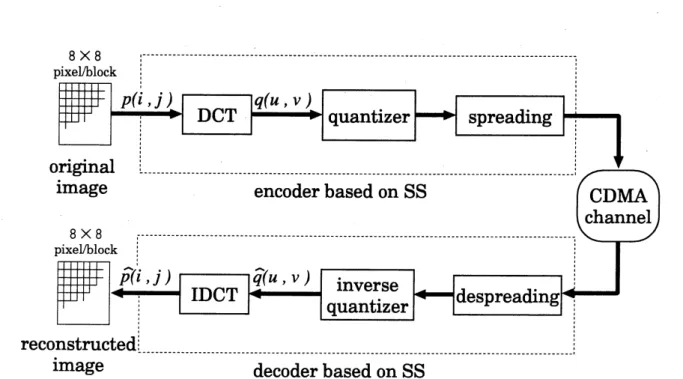
$[13],[14]$A basic inlage $\mathrm{c}\mathrm{o}\mathrm{m}\mathrm{m}11\mathrm{n}\mathrm{i}\mathrm{c}\mathrm{a}\mathrm{t}\mathrm{i}_{\mathrm{o}\mathrm{n}}\mathrm{s}\mathrm{y}_{\mathrm{S}\mathrm{t}}\mathrm{e}\mathrm{n}1$ llsing spread spectrum technique is illustrated in $\mathrm{F}\mathrm{i}\mathrm{g}_{11}\mathrm{r}\mathrm{e}8$. First, images are
$1$)
$\mathrm{a}\mathrm{r}\mathrm{t}\mathrm{i}\mathrm{f}\mathrm{i}\mathrm{o}\mathrm{n}\mathrm{e}\mathrm{d}$ into small blocks ($8\cross 8$ pixels), and the discrete cosine transfornl (DCT) of$\mathrm{t}\mathrm{w}\mathrm{o}^{-}\mathrm{d}\mathrm{i}\mathrm{l}\mathrm{n}\mathrm{e}\mathrm{n}\mathrm{s}\mathrm{i}\mathrm{o}\mathrm{n}\mathrm{a}1$(2-D) signal
$p(\dot{\uparrow},j)$ in each block is computed.
$\mathrm{N}e\mathrm{x}\mathrm{t}$ the 2-D DCT coefficients $q(?l, v)$ are quantized and appropriate nunlbers of bits are
assigned to them. Note that encoding and decoding are implemented $\mathrm{b}1\mathit{0}$ck by block.
The DCT coefficients are nlllnbered as shown in Figure
9.
We assignmore
bits to low$\mathrm{f}\mathrm{r}\mathrm{e}\mathrm{q}_{1}1e\mathrm{n}\mathrm{c}\mathrm{y}$ coefficients than to high ones. The bit allocation map we use is shown in Figure
10. $\mathrm{U}^{i^{\vee}}\mathrm{e}$ transmit only the first 15 DCT coefficients. nanlely
$54\mathrm{b}\mathrm{i}\mathrm{t}\mathrm{s}/\mathrm{b}\mathrm{l}\mathrm{o}\mathrm{c}\mathrm{k},$ $0.84\mathrm{b}\mathrm{i}\mathrm{t}/\mathrm{p}\mathrm{i}\mathrm{x}\mathrm{e}\mathrm{l}$.
Fllrtherll)ore. the $7?$-th ssignificant bit of the m-th coefficient $q_{m}$ is denoted by $q_{m-n}$, for
exalnple. $q_{0-1}$ is the most significant bit (MSB) of the DCT coefficient $q_{0}$ and $q_{0-_{8}}$ is the
least significant bit (LSB). In this paper. agray-scale$\mathrm{i}_{111}\mathrm{a}\mathrm{g}\mathrm{e}(8\mathrm{b}\mathrm{i}\mathrm{f}\mathrm{S}$ per pixel. $720\cross 576$ Pixels, $\cdot$
Figure 8: Illlage $\mathrm{C}\mathrm{o}\mathrm{m}111\mathrm{u}\mathrm{n}\mathrm{i}_{\mathrm{C}}\mathrm{a}\mathrm{f}\mathrm{i}\mathrm{o}\mathrm{n}\mathrm{s}\mathrm{y}\mathrm{S}\mathrm{f}\mathrm{e}\mathrm{l}\mathrm{l}\mathrm{l}$using SS techniques.
Figure 9: Coefficient nunlbers. $\mathrm{F}\mathrm{i}\mathrm{g}_{11}\mathrm{r}\mathrm{e}10$: Bit allocation lnap.
Figure 11: The original image ((
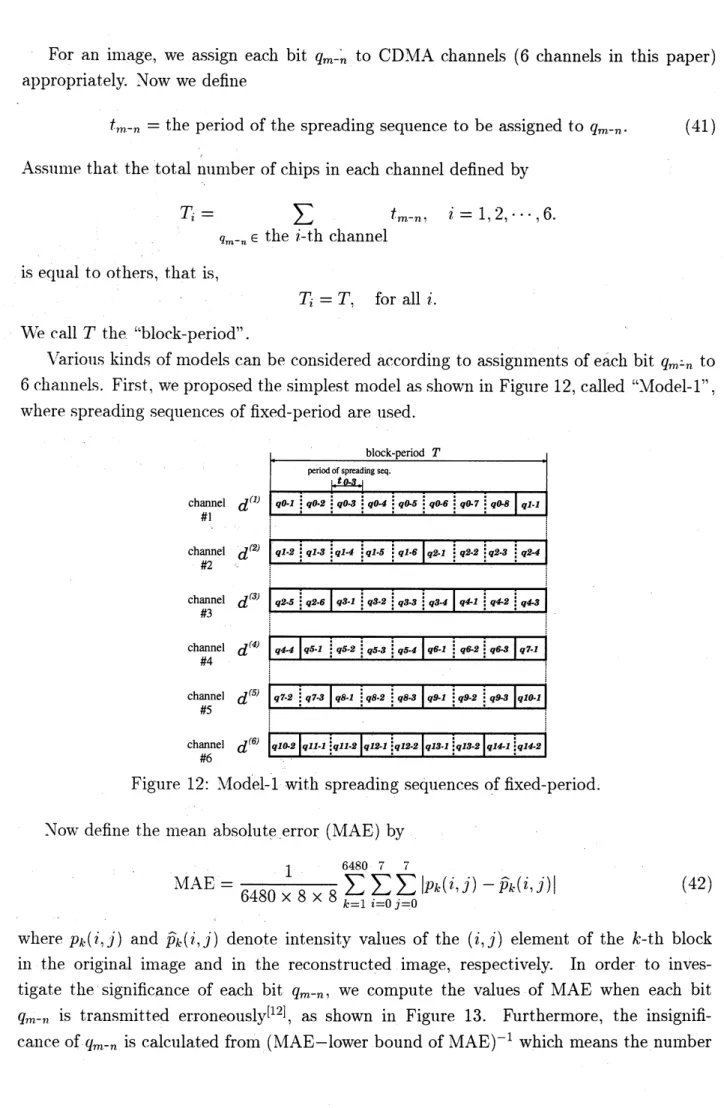
For an image, we assign each bit $q_{m^{-}n}$ to CDMA channels (6 channels in this paper)
appropriately. Now we define
$t_{m- n}=\mathrm{t}\mathrm{h}\mathrm{e}$ period of the spreading sequence to be assigned to
$q_{m^{-}n}$. (41)
$\mathrm{A}_{\mathrm{S}\mathrm{S}1}1111\mathrm{e}$ that the total $\mathrm{n}\iota \mathrm{l}\mathrm{n}\mathrm{l}\mathrm{b}\mathrm{e}\mathrm{r}$ of
chips in each channel defined by
$T_{i}=$ $\sum$ $t_{m-n}$. $i=1,2,$ $\cdots,$$6$.
$q_{m^{-}n}\in \mathrm{t}\mathrm{h}\mathrm{e}$ i-th channel
is equal to others, that is,
$T_{i}=T$. for all $i$.
We call $T$ the “block-period”
Various kinds of models can be considered according to $\mathrm{a}_{\mathrm{A}}\mathrm{s}\mathrm{s}\mathrm{i}\mathrm{g}\mathrm{n}\mathrm{n}\mathrm{l}\mathrm{e}\mathrm{n}\mathrm{t}\mathrm{S}$ofeach bit
$q_{m-n}\sim$ to
6 channels. First. weproposed the sinlplest model as shown in Figure 12, called]‘Model-l”,
where spreading sequences offixed-period are used.
chann#lel
$d^{(l)}.\ovalbox{\tt\small REJECT}_{q\mathit{0}\mathit{1}:}:::q\mathit{0}z:q\mathrm{p}\mathrm{c}\mathrm{r}\mathrm{i}\mathrm{o}\mathrm{d}\circ \mathrm{f}\mathrm{s}\mathrm{p}m\mathit{0}St\mathrm{d}\mathrm{m}\mathrm{g}\mathrm{s}_{4:}:q\mathit{0}\mathrm{b}1_{0}\mathrm{c}\mathrm{k}\mathrm{p}\mathrm{e}\mathrm{r}\mathrm{i}\mathrm{o}\mathrm{d}\mathrm{c}\mathrm{q}:q\alpha \mathit{5}:\mathit{0}:^{q}::T\delta:_{q}\mathit{0}7:q\mathit{0}\mathit{8}q\mathit{1}\mathit{1}|$channel $d^{(2)}$ $n$ $\mathrm{c}\mathrm{h}\mathrm{a}\mathrm{n}\mathrm{n}\mathrm{e}\mathrm{l}\# 3d^{(\mathit{3}J}$ $\mathrm{c}\mathrm{h}\mathrm{a}\mathrm{n}\mathrm{n}\mathrm{e}\mathrm{l}\# 4d^{(\mathit{4})}$ : $\mathrm{c}\mathrm{h}\mathrm{a}\mathrm{n}\mathrm{n}\mathrm{e}\mathrm{l}\# 5d^{(\mathit{5}J}$ $\mathrm{c}\mathrm{h}\mathrm{a}\mathrm{n}\mathrm{n}\mathrm{e}\mathrm{l}\# 6d^{(\mathit{6}J}$ .
Figure 12: Model-l with spreading sequences offixed-period.
Now define the mean absolute error (MAE) by
MAE $= \frac{1}{6480\cross 8\cross 8}\sum_{k=1}^{8}\sum_{=i0j}\sum_{0}^{\overline{/}}6407=|p_{k}(i,j)-\hat{p}_{k}(i, j)|$ (42)
where $p_{k}(i,j)$ and $\hat{p}_{k}(i,j)$ denote intensity values of the $(i, j)$ element of the k-th block
in the original $\mathrm{i}_{1}\mathrm{n}\mathrm{a}\mathrm{g}\mathrm{e}$ and in the reconstructed image, respectively. In order to
inves-tigate the significance of each bit $q_{m-n}$, we compute the values of MAE when each bit
$q_{m-7?}$ is transmitted $\mathrm{e}\mathrm{r}\mathrm{r}\mathrm{o}\mathrm{n}\mathrm{e}\mathrm{o}\mathrm{u}\mathrm{S}\mathrm{l}\mathrm{y}^{[1]}\underline’$ , as shown in Figure 13. Furthermore, the
insignifi-cance of$q_{m- n}$ is calculated $\mathrm{f}\mathrm{r}\mathrm{o}\ln$
of the erroneously transmitted bit $q_{m- n}$ to
cause a
constant MAE,as
shown in Figure14.
Figure 13: MAE when each bit $q_{m^{-}n}$ is trans- Figure 14: Insignificance of the bit
$q_{m-n}$,
nlitted erroneously. namely. the nunlber of erroneously
translnit-ted bits $q_{m^{-}n}$ to cause a constant MAE.
period of spreadingsequences
Figure 15: Bit error rates in asynchronous CDMA systems using Chebyshev bit sequences.
Model-l is not efficient because $\mathrm{e}\mathrm{a}\mathrm{C}_{\text{ノ}}\mathrm{h}$bit
$q_{m- n}$ is equiprobably transmitted in error. As
is well known. for a constant $\mathrm{n}\mathrm{l}\mathrm{l}\mathrm{n}\mathrm{l}\mathrm{b}\mathrm{e}\mathrm{r}$ofchannels, spreading sequencesof longer periods can
reduce bit error rates than ones of shorter periods. This motivates us to assign spreading
$\mathrm{s}\mathrm{e}\mathrm{q}_{11\mathrm{e}}\mathrm{n}\mathrm{c}e\mathrm{S}$ ofan appropriate period to the bit $q_{m- n}$ according to its significance. To do this,
we should investigate the bit error rates for various periods of spreading sequences and for
“Chebyshev bit $\mathrm{s}\mathrm{e}\mathrm{q}\mathrm{u}\mathrm{e}\mathrm{n}\mathrm{c}\mathrm{e}\mathrm{s}^{15}$]” which are generated by the Chebyshev lllap, Such sequences
are quite different from LFSR
sequences
such as $\mathrm{h}\mathrm{I}$sequences,
$\mathrm{I}\backslash ^{r}\mathrm{a}\mathrm{S}\mathrm{a}\mathrm{n}\mathrm{l}\mathrm{i}$sequences,
and Gold$\mathrm{s}\mathrm{e}\mathrm{q}\mathrm{u}\mathrm{e}\mathrm{n}\mathrm{c}\mathrm{e}\mathrm{s}^{[]}1$. Wehave alreadycalculated the bit error rates for the Chebyshev bit sequences
as
shown in Figure15.
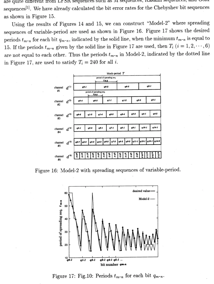
Using the results of Figures 14 and 15, we can construct “Mode1-2” where spreading
sequences ofvariable-period are used as shown in Figure 16. Figure
17
shows the desiredperiods$t_{\mathfrak{m}-n}$ for each bit $q_{m-n,}$. indicatedbythe solid line, when the nuinimum$tm-_{n}$ is equal to
15. If the periods $t_{m- n}$ given by the solid line in Figure 17 are llsed, then $T_{i}(i=1,2, \cdots, 6)$
are not equal to each other. Thus the periods $t_{m- n}$ in Mode1-2. indicated by thedotted line
in Figure 17. are used to satisfy $T_{i}=240$ for all $i$.
Figure 16: Mode1-2 with spreading sequences ofvariable-period.
6.2
Computer
Simulation
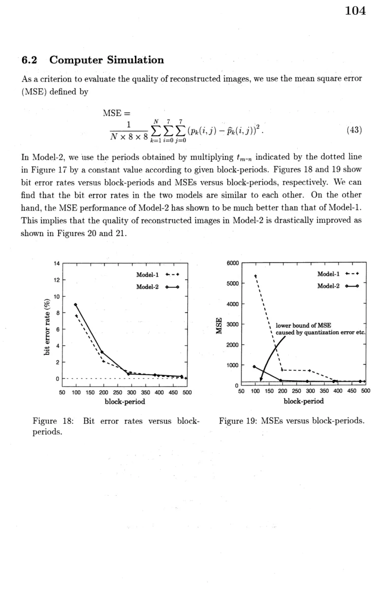
As a$\mathrm{c}\mathrm{r}\mathrm{i}\mathrm{t}_{l}\mathrm{e}\mathrm{r}\mathrm{i}\mathrm{o}\mathrm{n}$ to evaluate the qualityofreconstructed images, we use the
mean
square error(MSE) defined by
MSE $=$
$\frac{1}{N\cross 8\cross 8}\sum_{k=1i}^{N}\sum_{0=j}^{l}’\sum^{7}=0(pk(i,j)-\hat{p}k(i.j’))^{2}$ (43)
In $\mathrm{M}\mathrm{o}\mathrm{d}\mathrm{e}1-2_{\mathrm{t}}$. we use the periods obtained by multiplying $t_{m^{-}n}$ indicated by the dotted line
in Figure 17 by a constant value according to given block-periods. Figures 18 and 19 show
bit error rates versus block-periods and MSEs versus block-periods, respectively. We can
find that the bit error rates in the two models are silnilar to each other. On the other
hand. the MSE perforlnanceof Mode1-2 has shown to be much better than that ofModel-l.
Thisimplies that the quality of reconstructed images in Mode1-2 is drastically improved as
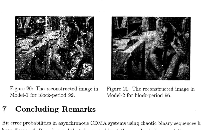
shown in $\mathrm{F}\mathrm{i}\mathrm{g}_{11\mathrm{r}}\mathrm{e}\mathrm{s}20$and 21.
$\mathrm{O}\mathrm{l}\mathrm{O}\mathrm{C}\mathrm{K}^{-}\mathrm{p}\mathrm{e}\mathrm{r}\mathrm{l}\mathrm{o}\mathfrak{a}$ block-penod
Figure 18: Bit error rates versus block- Figure 19: MSEs versus block-periods.
Figure 20: The reconstructed image in Figure 21: The reconstructed image in
Model-l for block-period 99. Mode1-2 for block-period 96.
7
Concluding
Remarks
Bit error probabilities in asynchronous CDMA$\mathrm{s}\mathrm{y}_{\mathrm{S}}\mathrm{t}\mathrm{e}\mathrm{n}1\mathrm{s}$using chaotic binary sequences have been discussed. It is observed that the central limit theorem holds for correlation values of
chaotic bit sequences. This enable us to theoretically estinlate such bit error probabilities.
Since the central limit theorenl $\mathrm{d}_{0}\mathrm{e}\mathrm{S}\mathrm{n}\mathrm{t}$ hold for LFSR sequences such as Gold sequences,
as shown in Fig.5, it is difficult to theoretically estimate the bit error probabilities in the
systenl using LFSR sequences. However, it is noteworthy that the bit error probabilities
for chaotic bit sequences are capable of estimating the ones for Gold sequences when the ntlnlber of channels is large.
Furtheremore, inlage conlmunication systems using CDMA channels with spreading
se-$\mathrm{q}\iota \mathrm{l}\mathrm{e}\mathrm{n}\mathrm{c}\mathrm{e}\mathrm{S}$of variable-period are proposed. We have given an efficient method for assigning
periods of spreading sequences based on the insignificance of each bit of DCT coefficients.
The CDMA systems using spreading sequences of variable-period have the following
ad-vantages: 1) The quality of reconstructed images are drastically improved within a linlited
bandwidth; and hence 2) The bandwidth is not so much for the transmission of images.
Note that such techniques can be also applied to color inlage communications.
References
[1] D. V. Sarwate and M. B. Pursley, (‘Crosscorrelation properties of $\mathrm{p}\mathrm{s}\mathrm{e}\mathrm{u}\mathrm{d}_{\mathrm{o}\mathrm{r}\mathrm{a}\mathrm{n}}\mathrm{d}_{0}\mathrm{n}1$and
related sequences,” Proc. IEEE. Vol.68, no.3, pp.593-619. 1980.
[2] Jackson. E. Atlee, Perspective nonlinear dynamics, Cambridge Univ. Press, 1989.
[4] R. L. Adler and T. J. Rivlin, “Ergodic and mixing properties of Chebyshev
polynomi-als,” Proc. Amer.Math.Soc., vol.15, pp. 794-796,1964.
[5] T.Kohda and A.Tsuneda, “Pseudonoise Sequence by Chaotic Nonlinear Maps and
Their Correlation $\mathrm{P}_{\Gamma 0_{\mathrm{P}}}\mathrm{e}\mathrm{r}\check{\mathrm{t}}\mathrm{i}\mathrm{e}\mathrm{s},$” IEICE Trans. on Communications, vol.E76-B, no.8,
855-862,
1.9.93.
[6] William Feller, An Introduction to Probability Theory and Its Applications, vol.2, John
Wiley&Sons,
1966.
$[\overline{(}]$ N. $\mathrm{M}\mathrm{a}\mathrm{c}\mathrm{D}_{\mathrm{o}\mathrm{n}}\mathrm{a}\mathrm{l}\mathrm{d}$, “Transmission ofcompressedvideo over radio $1\mathrm{i}\mathrm{n}\mathrm{k}’,$’ Visual
Communi-cation and Image Processing ’92, No.1818-149. 1992.
[8] W. F. Schreiber, ’‘Spread-Spectrum Television $\mathrm{B}\mathrm{r}\mathrm{o}\mathrm{a}\mathrm{d}_{\mathrm{C}}\mathrm{a}\mathrm{S}\mathrm{t}\mathrm{i}\mathrm{n}\mathrm{g},’$
’ SMPTE Journal,
pp.538-549. August.
1992.
[9] N. Doi. T. Yano, N. Kobayashi, H. Kishida, and M. Ohnishi, “Development ofWireless
$\mathrm{T}\mathrm{V}$-phones using Spread-Spectrunl $\mathrm{C}_{\mathrm{o}\mathrm{m}\mathrm{m}\mathrm{u}\mathrm{n}}\mathrm{i}\mathrm{C}\mathrm{a}\mathrm{t}\mathrm{i}_{0}\mathrm{n}_{c}.$” Proc. The 16th $\mathrm{S}\mathrm{y}\mathrm{n}\mathrm{u}\mathrm{p}_{0}\mathrm{S}\mathrm{i}\mathrm{u}\ln$on
Infornlation Theory and Its Applications (SITA ’93). pp.121-124, 1993.
[10] M. K. Simon, J. K. Olnura, R. A. Scholtz, and $\mathrm{B}.\mathrm{K}$.Levitt. Spread Spectrum
Commu-nications Handbook. $\mathrm{M}\mathrm{c}\mathrm{G}\mathrm{r}\mathrm{a}\mathrm{w}$-Hill.
1994.
[11] R. L. Peterson. R. E. Ziemer, and D. E. Borth, Introduction to SpreadSpectrum
Com-munications, Prentice-Hall,
1995.
[12] Y. $\mathrm{I}\backslash ^{r}\mathrm{o}\mathrm{y}\mathrm{a}\mathrm{n}\mathrm{l}\mathrm{a}$ and S. Yoshida, “StillImage Transmission using ARQ
over
Fading Channel”, Proc. the 17th Symposiumon Information Theory and Its Applications, pp.257-260,
1994.
[13] T. Kohda, A. $\mathrm{T}_{\mathrm{S}1\ln}\mathrm{e}\mathrm{d}\mathrm{a}$, A. Osiunli and K. Ishii, ’‘A study on pseudonoise-coded ilnage
$\mathrm{c}\mathrm{o}\mathrm{n}\mathrm{l}\mathrm{n}\mathrm{l}\mathrm{u}\mathrm{n}\mathrm{i}\mathrm{C}\mathrm{a}\mathrm{t}\mathrm{i}\mathrm{o}\mathrm{n}\mathrm{s}$” Proc. of SPIE’s Visual Communications and Inlage Processing ’94,
pp.874-884, 1994.
[14] T. Kohda, K. Ishii, and A. Tsuneda, $‘ i\mathrm{I}\mathrm{m}\mathrm{a}\mathrm{g}\mathrm{e}$ Transmission Systems through CDMA
Channels Using Spreading Sequences of Variable-Period”, Proc. of IEEE Fourth
In-ternational $\mathrm{S}\mathrm{y}_{1}\mathrm{n}\mathrm{p}\mathrm{o}\mathrm{s}\mathrm{i}_{1}1\mathrm{m}$