The Limiting Behavior of Fuzzy States in Dynamic Fuzzy Systems (Dynamic Decision Systems under Uncertain Environments)

(1)

The

Limiting

Behavior of Fuzzy States

in

Dynamic Fuzzy Systems

北九州大学経済学部吉田祐治 (Yuji YOSHIDA)

1. Introduction and

notations

The limiting behavior of fuzzy states in dynamic fuzzy systems has been studied by

Kurano et al. [4] and Yoshida et al. [7]. Under a contractive condition for the fuzzy

relation, [4] showed that the limiting fuzzy state is a unique solution of a fuzzy relational

equation. Also, [7] discussed the limit theorem in a monotone case. In this paper, we

consider the limit theorem when fuzzy relations satisfy the transitive property. We show

that, in this case, the limiting fuzzy state is a solution of the fuzzy relational equation.

But the equation does not necessarily have a unique solution similarly to the monotone

case, therefore we need to investigate the space of the solutions of the equation.

The _{existence and the uniqueness of the solutions of the fuzzy relational equation has}

been studied by Kurano et al. [5] under some assumptions. In the transitive case, this

paper makes clear the structure of the space of the solutions of the fuzzy relational

equa-tion, and wegive a simple characterizationof the limiting fuzzy state by the fundamental

solutions for the numerical calculation of the limiting fuzzy state.

We use some notations in [5]. Let $E$ be a compact metric space. Let _$C(E)$ be the

collection of all non-empty closed subsets of $E$, and let $\rho$ be the Hausdorff metric on

$C(E)$

.

Then it is well-known ([3]) that $(C(E), \rho)$ is a compact metric space. Let $\mathcal{F}(E)$

be the set of all fuzzy sets $\tilde{s}$ :

$Earrow[0,1]$ which are upper semi-continuous _{and satisfy}

$\sup_{x\in E}\tilde{s}(x)=1$

.

For $\tilde{s}\in \mathcal{F}(E)$, the $\alpha$-cut $\tilde{s}_{\alpha},$ $\alpha\in[0,1]$, is defined by

$\tilde{s}_{\alpha}:=\{x\in E|\tilde{s}(x)\geq\alpha\}(\alpha\neq 0)$ and _{$\tilde{s}_{0}:=\mathrm{c}1\{x\in E|\tilde{s}(x)>0\}$},

where cl means the closure of a set. Let $\tilde{q}$ : $E\cross Earrow[0,1]$ be a fuzzy relation on $E$

satisfying $\tilde{q}(x, \cdot)\in \mathcal{F}(E)$ for $x\in E$

.

A fuzzy relation $\tilde{q}$is called “transitive” (see Klir and

Yuan [2]$)$ if it satisfies

$\tilde{q}(x, y)\geq\sup_{z\in E}\{\tilde{q}(X, Z)\wedge\tilde{q}(Z, y)\}$ , $x,$ $y\in E$

.

Throughout this paper, we assume $\tilde{q}$ is transitive. In Sections 1 and 2, we consider the

space of solutions $\tilde{p}\in \mathcal{F}(E)$ of thefollowing fuzzy relational equation (see [5]) :

$\tilde{p}(y)=\sup_{Ex\epsilon}\{\tilde{p}(x)\wedge\tilde{q}(X, y)\}$, $y\in E$, (1)

where $a$ A $b:= \min\{a, b\}$ for real numbers $a$ and $b$

.

By the solutions of (1) (see _{$[4, 7]$} for

$\mathrm{c}\mathrm{o}\mathrm{n}\mathrm{t}\mathrm{r}\mathrm{a}\mathrm{c}\mathrm{t}\mathrm{i}\mathrm{V}\mathrm{e}/\mathrm{m}\mathrm{o}\mathrm{n}\mathrm{o}\mathrm{t}\mathrm{o}\mathrm{n}\mathrm{e}$ fuzzy relations), in Section 3 we discuss the limiting behavior of

the sequence of fuzzy states $\{\tilde{s}_{n}\}_{n=}^{\infty}0\subset \mathcal{F}(E)$ with an initial fuzzy state _{$\tilde{s}\in \mathcal{F}(E)$} which

is defined by

$\tilde{s}_{0}:=\tilde{s}$, and

(2)

Crisp sets $\tilde{q}_{\alpha}(x)(x\in E, \alpha\in[0,1])$ are defined by

$\tilde{q}_{\alpha}(X):=\{$

$\{y\in E|\tilde{q}(x, y)\geq\alpha\}$ for $\alpha\neq 0$

$\mathrm{c}1\{y\in E|\tilde{q}(x, y)>0\}$ for $\alpha=0$.

In this paper, we assume the map $\tilde{q}_{\alpha}(\cdot)$ : $E[]arrow C(E)$ is continuous for all $\alpha\in[0,1]$. We

also define $\tilde{q}_{\alpha}(D):=\bigcup_{x\in D}\tilde{q}\alpha(X)$ for $D\in C(E)$, and then we note that $\tilde{q}_{\alpha}$

:

$C(E)arrow C(E)$

.

For $x\in E$ and $\alpha\in[0,1]$, a sequence $\{\tilde{q}_{\alpha}^{n}(x)\}_{n}^{\infty}=0\subset C(E)$ is defined iteratively by

$\tilde{q}_{\alpha}^{0}(x):=\{x\}$, and $\tilde{q}_{\alpha}^{n+1}(x):=\tilde{q}_{\alpha}(\tilde{q}_{\alpha}(nX))$, $n=0,1,2,$ $\cdots$

.

Then we have the following lemma for a sequence of fuzzy relations $\{\tilde{q}^{n}\}_{n=1}^{\infty}$ defined by

$\tilde{q}^{1}:=\tilde{q}$, and

$\tilde{q}^{n+1}(x, y):=\sup_{z\in E}\{\tilde{q}^{n}(x, z)\wedge\tilde{q}(z, y)\}$, $x,$$y\in E$ for $n=1,2,$ $\cdots$

.

(3)

Lemma 1.1. The following (i) and (ii) hold:

(i) For all $n=1,2,$$\cdots$,

$\tilde{q}^{n}(x, y)\geq\tilde{q}(n+1x,y)$, _$x,$_{$y\in E$}, (4)

and

$\tilde{q}_{\alpha}^{n+1}(X)\subset\tilde{q}_{\alpha}^{n}(x)$, $x\in E,$ $\alpha\in[0,1]$

.

(5)

(ii) $\tilde{q}^{n}(x, x)=\tilde{q}(x, x)$ for all $x\in E$ an$dn=1,2,$$\cdots$ .

Let

$R_{\alpha}:=\{x\in E|x\in\cup^{\infty}n=1\tilde{q}_{\alpha}(nX)\}$ , $\alpha\in[0,1]$

.

Each state of $R_{\alpha}$ is called “$\alpha$-recurrent” (see [8]). From Lenuna l.l(i), we have

$R_{\alpha}=\{x\in E|\tilde{q}(X, X)\geq\alpha\}$, $\alpha\in(0,1]$. (6)

Let $x\in E$

.

The following crisp sets are used in [5] to analyze the solutions of (1):

$F_{\alpha}(x):= \bigcup_{n=0}^{\infty}\tilde{q}^{n}\alpha(x)$,

and

$\hat{F}_{\alpha}(x):=,\bigcap_{\alpha<\alpha}\mathrm{c}1\{F_{\alpha’}(X)\}(\alpha\neq 0)$ and

$\hat{F}_{0}(x):=\mathrm{c}1\{F_{0}(X)\}$

.

In the transitive case, by Lemma l.l(i) they are reduced to the following (7):

$\hat{F}_{\alpha}(x)=\{x\}\cup\tilde{q}_{\alpha}(x)$, _{$x\in E,$} $\alpha\in[0,1]$

.

(7)

Especially we have

$\hat{F}_{\alpha}(z)=\tilde{q}_{\alpha}(z)$, _{$z\in R_{1},$} $\alpha\in[0,1]$

.

(8)

Therefore, we obtain the following lemma.

(3)

(i) For$\tilde{p}\in \mathcal{F}(E),\tilde{p}$ satisfies (1) ifand only if

$\tilde{q}_{\alpha}(\tilde{p}_{\alpha})=\tilde{p}\alpha$

’ $\alpha\in[0,1]$

.

(9)

(ii) Let $z\in R_{1}$

.

Defin$e$ a fuzzy state

$\tilde{p}^{z}(x):=\sup_{\alpha\in 10,1]}\{\alpha\wedge 1_{\hat{F}_{\Phi}(}z)(X)\}=\tilde{q}(_{Z,x})$, $x\in E$. (10)

Then $\tilde{p}^{z}\in \mathcal{F}(E)$ satisfies (1).

2. The

space of

the

solutions

We put $\mathcal{P}:=$

{

$\tilde{p}\in \mathcal{F}(E)|\tilde{p}$ is a solution of (1)}. Then the space $\mathcal{P}$ has the following

property:

Lemma 2.1 (Kurano et al. [5, Theorem $2.2(\mathrm{i}\mathrm{i})]$). Let $\tilde{p}^{k}\in P(k=1,2, \cdots, l)$, an$d$ let

$\{\alpha^{k}\in[0,1]|k=1,2, \cdots, l\}$ satisfy $\sup_{k=1,2,\cdots,l}\alpha^{k}=1$

.

Pu$t$

$\tilde{p}(x):=k=1,2\max,\cdots,\{l\alpha^{k}\wedge\tilde{p}^{k}(x)\}$, $x\in E$

.

(11)

Then $\tilde{p}\in \mathcal{P}$.

The purpose of this section is to prove an inverse of the statement of Lemma 2.1.

Namely, we represent general solutions $\tilde{p}\in P$ of (1) by the fundamental solutions $\tilde{p}^{z}$ of

(10). From now on, we assume $R_{1}\neq\emptyset$

.

We identify the states of $R_{1}$ with respect to the

following equivalent $\mathrm{r}\mathrm{e}\mathrm{l}\mathrm{a}\mathrm{t}\mathrm{i}_{0}\mathrm{n}\sim \mathrm{o}\mathrm{n}R_{1}$ (see [5] and (8)): For

$z_{1},$$z_{2}\in R_{1}$,

$z_{1}\sim z_{2}$ means that $z_{1}\in\tilde{q}_{1}(z_{2})$ and $z_{2}\in\tilde{q}_{1}(z_{1})$

.

Then we put $R_{1}^{\sim}:=R_{1}/\sim$

.

Assumption A. Let $\alpha\neq 0$ and _{$A\in C(E)$}

.

If$\tilde{q}_{\alpha}(A)=A$ holds, then

$R_{\alpha}\cap A\subset\cup\tilde{q}\alpha(zz\in R_{1}\sim_{\mathrm{n}}A)$

.

From now on, we suppose that Assumption A holds ($\mathrm{c}.\mathrm{f}$. _$[5$, Assumption A3]).

Theorem 2.1. Let $\tilde{p}$ be a $sol\mathrm{u}$tion of (1). Then, there exists a family of coefficients

$\{\alpha^{z}\in[0,1]|z\in R_{1}^{\sim}\}$ satisfying _{$\sup_{z\in R_{1}^{\sim\alpha^{z}}}=1$} and

(4)

3. A

Limit

Theorem

We uses the convergency of fuzzy states in following sense.

Definition (see [7]). Let $\tilde{s}_{n},\tilde{p}\in \mathcal{F}(E)$

.

Then

$\lim_{narrow\infty}\tilde{s}_{n}=\tilde{p}$ means $\rho(\tilde{s}_{n,\alpha},\tilde{p}_{\alpha})arrow \mathrm{O}$ $(narrow\infty)$ for all $\alpha\in[0,1]$,

where $\tilde{s}_{n,\alpha}$ are the $\alpha$-cuts of $\tilde{s}_{n}$ and

$\rho$ is the given Hausdorff metric.

Fix an initial fuzzy state $\tilde{s}\in \mathcal{F}(E)$. In this section, first we discuss the convergence

of the sequence of fuzzy states $\{\tilde{s}_{n}\}_{n=}^{\infty}0$ defined by (2), and we prove the limiting fuzzy

state is a solution of the fuzzy relational equation (1). Next, we give a representation of

the limiting fuzzy state for the numerical calculation, by using the characterization (12).

Lemma 3.1. Let $\alpha\in[0,1]$

.

Then

$\lim_{narrow\infty}\tilde{s}_{n},\alpha=\cap n\geq 1x\in\cup\tilde{S}\alpha\tilde{q}^{n}\alpha(_{X})=x\in\bigcup_{\overline{s}_{\alpha}n}\cap\tilde{q}\alpha(n)\geq 1x$

.

(13)

We use the following lemma to construct the limiting fuzzy state.

Lemma 3.2 ([4, 6]). Let a family ofsubsets $\{D_{\alpha}|\alpha\in[0,1]\}\subset C(E)$ satisfies the

followin$g$ condition$s(\mathrm{a})$ and $(b)$:

(a) $D_{\alpha}\subset D_{\alpha’}$ for $0\leq\alpha’<\alpha\leq 1$

.

(b) $\lim_{\alpha’\uparrow}\alpha D_{\alpha’}=D_{\alpha}$ for$\alpha\in(0,1]$.

Then $\tilde{s}(x):=\sup_{\alpha\in[0,1}]\{\alpha\wedge 1_{D_{\alpha}}(x)\},$ $x\in E$, satisfies $\tilde{s}\in \mathcal{F}(E)$ and $\tilde{s}_{\alpha}=D_{\alpha}$ for all $\alpha\in[0,1]$, where $1_{D}$ denotes the characteristicfunction ofa set $D\in C(E)$.

From Lemma 3.1, we define

$\tilde{p}(x):=\sup\{\alpha\wedge 1_{D_{\alpha}}(x)\}$, $x\in E$, (14)

$\alpha\in[0,1]$

where

$D_{\alpha}:= \lim_{narrow\infty}\tilde{s}n,\alpha=\bigcap_{n\geq 1x}\bigcup_{\alpha}\tilde{q}_{\alpha}(\epsilon\tilde{s}nX)=x\in\cup \mathrm{n}\tilde{q}_{\alpha}^{n}(x)\overline{S}\alpha n\geq 1$’

$\alpha\in[0,1]$

.

(15)

Theorem 3.1. $\tilde{p}h$as thefollowing property (i) and (ii):

(i) $\tilde{p}=\lim_{narrow\infty n}\tilde{S}\in \mathcal{F}(E)$

.

(ii) $\tilde{p}$ is a solution of (1).

Finally, by using the limit theorem (Theorem 3.1) and the characterization of the

solutions of the fuzzy relational equation$\vee(.\mathrm{T}\mathrm{h}\mathrm{e}\mathrm{o}\mathrm{r}\mathrm{e}\mathrm{m}2.1)$ , we give a simple representation

(5)

Theorem 3.2. The coefficients in Theorem 2.1 aregiven by

$\alpha^{z}=\tilde{q}(_{\tilde{S}})(Z)=\tilde{p}(Z)$, $z\in R_{1}^{\sim}$, (16)

where $\tilde{q}(\tilde{s})(z)=\sup_{x\in E}\{\tilde{\mathit{8}}(x)\wedge\tilde{q}(x, z)\}$. Namely,

$\tilde{p}(x)=\sup_{z\in R^{\sim}1}\{\tilde{q}(\tilde{S})(_{Z})\wedge\tilde{q}(z,x)\}=\sup_{1}\{\tilde{p}(Z)\wedge\tilde{q}z\epsilon R\sim(Z, x)\}$, $x\in E$. (17)

4. A

numerical

example

We consider a one-dimensional $\mathrm{n}\mathrm{u}‘ \mathrm{m}\mathrm{e}\mathrm{r}\mathrm{i}_{\mathrm{C}}\backslash$

‘al

example to

_illust.r

ate our results in Sections 2

and 3. Let $E=[-2,2]$

.

We give the transitive fuzzy relation $\tilde{q}$ (see Fig.1) by

$\tilde{q}(x, y)=$

’

$( \frac{j(y)+y-2x}{y-!(y)}0)\wedge 1$ if$xy>0,$ $y\neq-1,1$

1 if$y=0$

1 if $x\geq 1,$ _$y=1$ (18)

1 if $x\leq-1,$ $y=-1$

$\backslash 0$ otherwise,

where $f(y):=y^{5}-2y^{3}+2y$_, _{and we} _put $a \mathrm{O}:=\max\{a, 0\}$ and $a \wedge 1:=\min\{a, 1\}$ for

real numbers $a$

.

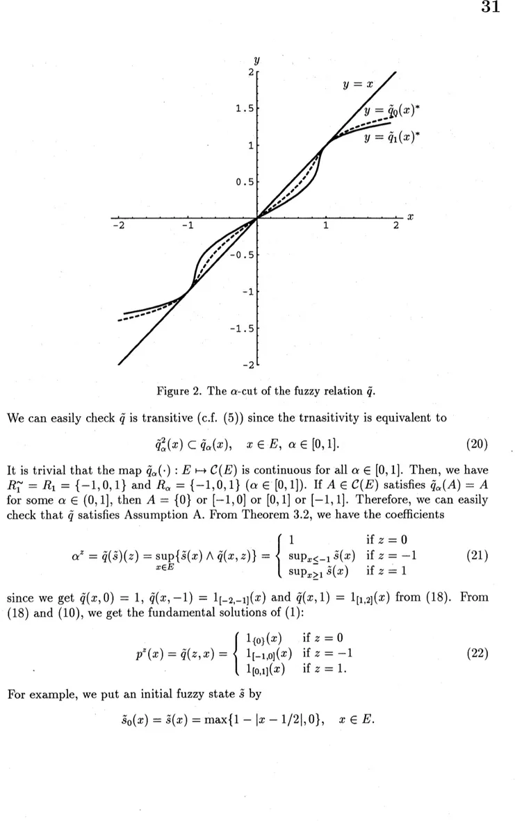
The $\alpha$-cut of fuzzy relation $\tilde{q}$ is written as follows (see Fig.2):

$\tilde{q}_{\alpha}(x):=\{$ $[0,\tilde{q}_{\alpha}(X)*]$ if $x\geq 0$ $[\tilde{q}_{\alpha}(x)^{*}, 0]$ if $x<0$, (19) where $\tilde{q}_{\alpha}(x)^{*}:=\{$ $\max\tilde{q}_{\alpha}(x)$ if $x\geq 0$ $\min\tilde{q}_{\alpha}(x)$ if $x<0$

.

(6)

Figure 2. The $\alpha$-cut ofthe fuzzy relation $\tilde{q}$

.

We can easily check $\tilde{q}$ is transitive $(\mathrm{c}.\mathrm{f}.$(5)$)$ since the trnasitivity is equivalent to

$\tilde{q}_{\alpha}^{2}(x)\subset\tilde{q}_{\alpha}(x)$, $x\in E,$ $\alpha\in[0,1]$

.

(20)

It is trivial that the map $\tilde{q}_{\alpha}(\cdot)$ : $Erightarrow C(E)$ is continuous for all $\alpha\in[0,1]$

.

Then, we have

$R_{1}^{\sim}=R_{1}=\{-1,0,1\}$ and $R_{\alpha}=\{-1,0,1\}(\alpha\in[0,1])$. If $A\in C(E)$ satisfies $\tilde{q}_{\alpha}(A)=A$

for some $\alpha\in(0,1]$, then _$A=\{0\}$ or $[$-1,$0]$ or $[0,1]$ or [-1, 1]. Therefore, we can easily

check that $\tilde{q}$ satisfies Assumption A. From Theorem 3.2, we have the coefficients

$\alpha^{z}=\tilde{q}(\tilde{S})(Z)=x\in E\mathrm{s}\mathrm{u}\mathrm{p}\{_{\tilde{S}}(x)\wedge\tilde{q}(x, z)\}=(\sup_{x\geq 1}\tilde{s}(_{X})\sup_{x\leq}1-1\tilde{s}(_{X)}$ $\mathrm{i}\mathrm{f}z\mathrm{i}\mathrm{f}_{\mathcal{Z}}=\mathrm{i}\mathrm{f}z=1=0-1$ (21)

since we get $\tilde{q}(x, 0)=1,\tilde{q}(x, -1)=1_{[]()}-2,-1x$ and $\tilde{q}(x, 1)=1_{[1,2]}(x)$ from (18). From

(18) and (10), we get the fundamental solutions of (1):

$p^{z}(x)=\tilde{q}(z,X)=\{$

1$\{0\}(x)$ if $z=0$

$1_{1-1,0}](X)$ if$z=-1$

$1_{1}0,1](x)$ if$z=1$

.

(22)

For example, we put an initial fuzzy state $\tilde{s}$ by

(7)

Then, from (21), we have $\alpha^{0}=1,$ $\alpha^{-1}=0$ and $\alpha^{1}=1/2$

.

By Theorem 3.1, the sequence

offuzzy states $\{\tilde{s}_{n}\}_{n}\infty=0$ converges to the the limiting fuzzy state $\tilde{p}$

.

Therefore, from (21),

(22) and Theorem 3.2, we obtain the the limiting fuzzy state

$\tilde{p}(x)=z=-1\max,\{\alpha^{z}\wedge 0,1p(zX)\}=1_{\{0\}(}X)\mathrm{v}\{1/2\wedge 1_{[0,1]}(x)\}=\{$

1 if $x=0$

1/2 if $0<x\leq 1$

$0$ otherwise.

References

[1] R.E.Bellman and L.A.Zadeh, Decision-making in a fuzzy environment, Management

Sci. Ser B. 17 (1970) 141-164.

[2] G.J.Klir and B.Yuan, Fuzzy Sets and Fuzzy Logic: Theory and Applications

(Prentice-Hall, London, 1995). Interscience Publishers, New York, 1958).

[3] K.Kuratowski, Topology I (Academic Press, New York, 1966).

[4] _{M.Kurano, M.Yasuda, J.Nakagami and Y.Yoshida, A limit theorem in some dynamic}

fuzzy systems, Fuzzy Sets and Systems 51 (1992) 83-88.

[5] M.Kurano, M.Yasuda, J.Nakagami and Y.Yoshida, A fuzzy relational equation in

dynamic fuzzy systems, to appear in Fuzzy Sets and Systems.

[6] V.Nov\’ak, Fuzzy Sets and Their Applications (Adam Hilder, Bristol-Boston, 1989).

[7] Y.Yoshida, M.Yasuda, _{J.Nakagami and M.Kurano, A limit theorem in some dynamic}

fuzzy systems with amonotone property, FuzzySets and Systems 94 (1998) 109-119.

[8] _{Y.Yoshida, The recurrence of dynamic fuzzy systems, to appear in Fuzzy} _Sets _and