東北大学機関リポジトリTOUR

(1)

A Quantitative Analysis of the Economic

Situation of Those Who Have Undergone Divorce:

The Gender Gap in Equivalent Household Income,

1998-2008, in Japan

著者

TANAKA Sigeto

(2)

(Anyone may quote from this paper within the boundary of the copyright law.) http://www.sal.tohoku.ac.jp/~tsigeto/11x.html International Sociological Association, Research Committee 06 (Committee on Family Research)

CFR Kyoto Seminar 2011 “Reconstruction of Intimate and Public Spheres in a Global Perspective” in Kyoto University, 2011.9.12 Kyoto

A Quantitative Analysis of the Economic Situation

of Those Who Have Undergone Divorce

The Gender Gap in Equivalent Household Income, 1998–2008, in Japan

TANAKA Sigeto

(Graduate School of Arts and Letters, Tohoku University)

Abstract

This paper addresses how marriage and divorce create gender inequality. It focuses on the economic situation of men and women after divorce, which constitutes the main component of the gender gap in the standard of living in contemporary Japan. The data are drawn from the National Family Research of Japan (NFRJ) project, in which family sociologists have repeatedly conducted large-scale surveys with national representative samples in the fiscal years 1998 (NFRJ98), 2003 (NFRJ03), and 2008 (NFRJ08). The datasets include 473 (NFRJ98), 494 (NFRJ03), and 463 (NFRJ08) respondents who had undergone divorce. The number of cases is thus adequate to obtain statistically reliable estimates through multivariate analysis. The author conducted a series of regression analyses to determine the effect of gender on the equivalent household income (i.e., household income divided by the square root of the number of people in the household) for divorced men and women, controlling for variables such as age, education, household composition, marital status, and employment status. The results reveal the powerful and persistent effects of the gender differences in the probability of maintaining one’s employment status as an ordinary regular employee and in the probability of co-residing with young children. These factors have perpetuated the disadvantageous post-divorce situation for women, while the situation of divorced men has been getting worse from 1998 through 2008. Another important factor is remarriage, from which men and women receive different economic outcomes. We will discuss the theoretical and political implications of the results, with a special attention to the recent family law debates over equity-oriented reforms in the system for financial provision on divorce.

Keywords: marital status, financial provision on divorce, discontinuous career, custody, remarriage

1. Introduction

Increasing divorce is one of the major social changes in Japan today. According to the 2005 Population Census, divorced (and remained single) people accounted for 5.4% (4.2% of men and 6.6% of women) of the population aged 25–69 (Table 1). The figure was lower in the past: 1.9% (1.2% of men and 2.6% of women) in 1975. Then it started to grow and has been almost tripled in these three decades. This change has been parallel to the increasing unmarried population. As a result of these changes, the proportion of married people has fallen to around 70% in 2005.

Divorce has thus been a common phenomenon nowadays. In addition, the figure above does not include those who remarried. The proportion of those who underwent divorce, including those who remarried, should be greater by some percent. If the figure will continue to grow, it is highly possible that in the near future, a large proportion of the Japanese population will undergo divorce, as Fukuda Nobutaka (2009) predicted.

(3)

This increasing divorce is to be subjected to an important concern from the perspective of gender equality, because there is a great gender gap in post-divorce living standards. However, although this fact has become a commonly accepted theory, there have not been sufficient scientific evidences. There has been a long debate among law scholars on equity-oriented reformation of the divorce system, without quantitative evidence for the effect of such reformation to achieve gender equality in post-divorce life. Recently, the Government of Japan has established the framework of gender-equal policies since late 1990s, but the impact of increasing divorce has been out of its focus. Research on post-divorce life has thus been inactive and understaffed.

In this paper, we aim at quantitative evidences on two critical questions about gender equality in post-divorce life.

Determination of the gender gap in economic situations by marital status and experiences Decomposition of the factors creating the gender gap after divorce

The aims have been derived from legal and policy-related concerns about gender equality — especially from the legal concern on the possible contribution of the equity-oriented reformation of the divorce system advocated by law scholars to lessen the gender gap.

2. Literature on Post-Divorce Life and Gender Gap

2.1. Quantitative approach to divorced people

In Japanese society, we have little literature of quantitative research on the economic gender gap in post-divorce life. There have been demographic works on the frequency of divorces and the determinants of divorce, including Vital Statistics1. However, they are not useful for our purpose, because they contain little detail on social and economic aspects of post-divorce life.

There have been a few sample surveys of divorced people. For instance, the Ministry of Health and Welfare (MHW 1999) conducted such a survey with a sample from the notifications of divorce submitted to the local governments. These data can be used to ascertain, to some degree, social and economic aspects of the post-divorce life at the time of the survey. However, since such surveys do not explore long-term change in economic status, the data are not helpful to trace the impact of social and economic positions prior to marriage, during the marital life, and after divorce. In addition, there have been few publications of findings from such surveys. On the bibliography published by National Institute of Population and Social Security Research (IPSS 2006: 153– 78; IPSS 2008: 147–54), which carries a huge list of recent publications on divorce in Japan, we can find no title related to gender gap in post-divorce life — although the judgment might be incorrect because it was based on the listed titles only.

2.2. Research of single-motherhood and the hypothesis of marital-life results

Under these circumstances, studies of single-mother households do provide some degree of data. Numerous researchers have conducted empirical studies on this topic, because single-mother households have been one of the major targets of social policy, as Iwata Masami (2005) pointed out. Most of these studies lack a perspective

1_{Vital Statistics, annually published by the Ministry of Health, Labour and Welfare, include a record of divorces notified to local}

governments. These statistics form a reliable and official source for the frequency of divorces and the basic demographic variables of divorced people.

(4)

of male-female comparison, as a natural result of focusing on female subjects only. However, some such research offers suggestions for exploring gender differences.

The Japan Institute of Labour (JIL 2003) conducted a project aiming at the secondary analysis of the official statistics to establish policies promoting the independence of mothers in single-mother households. As a part of this project, Nagase Nobuko (2004) presented a hypothesis on the conditions that cause economic problems for women after divorce as follows.

Many women quit regular employment and are not employed before the divorce Mothers tend to take custody of young children

It is difficult to forge a balance between work and childcare

Hamamoto Chizuka (2005), Kambara Fumiko (2006), Shinotsuka Eiko (1992), and Tamiya et al (2008) also suggested similar factors related to the economic difficulties of single-mother households.

Nagase (2004) implies that the post-divorce gender gap is created within the marital life before divorce. We accordingly refer to Nagase’s hypothesis as the hypothesis of “marital-life results”. If the hypothesis is true, we can regard the gap as caused by faults in the family system. As Gary S. Becker (1991) formalized, differences in human capital between spouses are due to the effort of specialization in marital life that is established to manage the household efficiently. We also mention responsibilities to provide for children, who themselves are an outcome of marital life. Divorcing couples shall make a fair settlement of their human capital and childrearing responsibilities on divorce. But they often fail to do so. Thereby gender differences emerge through the marital life, and consequently bring about the gender gap in the post-divorce life. The hypothesis of marital-life results thereby implies the gender inequality after divorce is primarily attributable to the marital life before divorce, although Nagase (2004) does not say so explicitly.

The hypothesis of marital-life results also suggests that the equity-oriented reformation of the divorce system could dramatically reduce the gender gap. Since the establishment of the provisions on the division of marital property under an amendment to the Civil Code (民法, 1947 Law No. 222), legal scholars2 have for many years asserted that financial provision on divorce should cover the husband’s or wife’s human capital and occupational status achieved through their cooperation. Recently, Suzuki Shinji (1992) clearly argued that spouse’s earning capacity should be subjected to an equitable division at divorce, if it was gained during marital life. Motozawa Miyoko (1998: 272–6) gives a comprehensive description of the principle and a practical standard for an equitable settlement. Motozawa’s standard calls for an equitable treatment of any changes that have occurred during marriage. That is, divorcing couples should restore any change to its original state (i.e., the state before marriage), as far as such restoration is feasible. And, if such restoration is unfeasible, they should provide monetary transfer to make an equitable settlement concerning the change. Motozawa also argues that such treatment includes the following three as typical cases.

Disadvantages in employment arising from specialization between husband and wife

Burdens related to the raising of their children, including the opportunity cost for an interrupted career or for shorter working hours

2_{See Tsuneta et al (1955) and Wagatsuma Sakae (1953) for the earliest advocators of the divorce system providing equitable}

(5)

Disease caused or worsened by the marital life.

Let us refer to the above new principle for financial provision on divorce as “equity-oriented”, because it is logically based on the idea of equitable division of marital properties on divorce. In practical consideration, however, both Suzuki (1992) and Motozawa (1998) interpret the principle as calling for equal division. This interpretation is in line with the recent trend about the divorce law, often called “2 分の 1 ルール” [the fifty-fifty rule], which calls an equal division of marital properties to avoid fruitless and harmful battle between divorcing couple. We can expect that the equity-oriented principle thus brings about an equal settlement of any difference caused by the marital life. As a matter of course, it will be able to nullify the economic disadvantage of women who have specialized in housework or childcare during their marital life.

2.3. Recent progress

The hypothesis of marital-life results was based on insufficient empirical grounds, at least at its starting point. Nagase (2004) reached to the hypothesis by inferences made through the comparison of data on single-mother households with other official statistics, without any evidence directly supporting the hypothesis.

A possible counterargument was that many single-mother households were impoverished due to the fact that disparities had already been developed during the process of human capital formation prior to marriage. In fact, a relatively large proportion of single-mother households are made up of those in which the mother has a low level of education, as Fujiwara Chisa (2005) argued. The large number of women who are impoverished after divorce could be due to the fact that divorce is concentrated among women suffering disadvantages in human capital formation prior to marriage. If so, we cannot think of the gender gap as a result of marital life; we should rather think of it as a result from the gender differences in pre-marriage factors.

Based on this point, Tanaka (2008; 2010) offered quantitative evidences for the hypothesis of marital-life results, directly analyzing the economic status after divorce using Japanese national representative data. The analyses were on equivalent household income of men and women after divorce. Data were drawn from different two projects: SSM2005-J (Tanaka 2008) and NFRJ03 (Tanaka 2010). The results of these analyses clarified that the post-divorce equivalent household income of women was 29% (Tanaka 2010) to 36% (Tanaka 2008) lower than that of men. Two variables had a major impact on the equivalent household income of divorced persons: (1) a continuous career as a regular employee and (2) the co-residence with one’s young children after divorce. These variables exerted a great effect after controlling the effect by the level of education. In addition, pre-marriage employment status did not exert a significant effect (Tanaka 2008). The results of these analyses support the hypothesis of marital-life results, indicating that changes in economic situations that arise during marriage lead to a post-divorce inequality in living standards.

3. The Question to Be Answered

The author set our goal in this paper as confirmation of the findings on the gender gap and its factors. The above-mentioned studies have reported stable results in a qualitative term, in favor of the hypothesis of marital-life results. However, these results are not stable in a quantitative term. The estimate values produced by the analyses differ widely. Therefore, we have not received reliable answers regarding the extent either (1) of the post-divorce economic gap between men and women, or (2) of the effects exerted by the factors influencing this gap. In this paper, we try to replicate the results of Tanaka (2008; 2010) using large-scale datasets from NFRJ.

(6)

4. Data

We use data from the 1999, 2004, and 2009 iterations of the National Family Research of Japan (NFRJ98, NFRJ03, and NFRJ08), conducted by the Japan Society of Family Sociology (Table 2). These are survey data from probability samples of Japanese nationals residing in Japan, using the self-administered questionnaire (home-delivery, leave-and-pick-up) method. Subjects were chosen through stratified two-stage probability sampling. These surveys, which focused on relations between family members and relatives, are characterized by their detailed questioning about marital history (including divorce), the attributes of individual children, and other family-related events.

Details for each dataset are in Table 2. The NFRJ98 and NFRJ03 datasets have been opened to the public through the Social Science Japan Data Archive (SSJDA), the University of Tokyo (survey number 0191 and 0517). The use of the NFRJ08 dataset has been closed to the members of the joint-use project (NFRJ08 研究会) of the Japan Society of Family Sociology.

NFRJ98/NFRJ03 respondents’ age ranged 28–77 (as of the end of 1998/2003). NFRJ08 respondents’ age ranged 28–72 (as of the end of 2008). In order to keep comparability among these three datasets, we truncate respondents over 72 years old from NFRJ98/NFRJ03 datasets. Thereby the age of the subject for our analysis ranges 28–72 for all three datasets.

Each survey collected data from a large sample of over 9,000 persons, which offers us an adequate size of subsample for the analysis on divorced people. The number of respondents who had undergone divorce is more than 400 for each dataset. We have thus ensured an enough number of cases to obtain statistically reliable estimates.

5. Income and Gender Gap

5.1. Equivalent household income

The main variable for the analyses below is the equivalent household income. It is a gauge widely used to capture people’s standards of living. This measure deflates household income by household size —by dividing income by the square root of the number of people in the household. Assuming that there are economies of scale in the management of household finances and that all members of the household receive an equal distribution of income, equivalent household income has traditionally been used as an approximate measure of individual standards of living (OECD 2001).

The NFRJ surveys asked about annual household income3 in the year previous to the survey. Respondents were required to select from pre-coded categories4 for their income level. The equivalent household income is calculated as Equation (1), with l denoting the lower and h denoting the upper limit of the selected income level (each in units of 10,000 yen), and n denoting the number of persons co-residing with the respondent (including the respondent).

3_{It is usual for approximation of living standards to measure disposable income after tax. Unfortunately, NFRJ questions measured}

incomes including tax, without information to exclude tax. This would make some biases for the following analyses.

4_{On the questionnaire, 9 categories are printed for NFRJ98, mostly separated in intervals of 2 million yen; 18 categories for}

NFRJ03, mostly separated in intervals of 1 million yen; 19 categories for NFRJ08, intervals are the almost same as NFRJ03. Note that respondents for NFRJ98 thus answered from less number of categories with wider intervals than for the other two surveys. In addition, there were some differences in the wording and the context for the question of household income among the questionnaires for three surveys. These differences may also reduce the comparability.

(7)

n

h

l

2 income

household

Equivalent

=

+

(1)

The highest category for measurement of household income was 12 million yen or more (NFRJ98) or 16 million yen or more (NFRJ03/NFRJ08). For calculation of Equation (1), we assigned 1400 (NFRJ98) or 1700 (NFRJ03/NFRJ08) to the upper limit h for these highest categories (in 10,000 yen).

The measure of equivalent household income derived in this equation has a skewed distribution. In the following analysis, we employ this measure converted using the natural logarithm to approximate a normal distribution. This conversion resulted in omission of a few cases with no household income (=0) from the following analyses, because logarithm cannot be defined for zero. The results will, however, appear in tables with the figures converted through exponential transformation (which is the reverse function of logarithm) for easier interpretation.

Table 3 shows the (geometric) mean values of equivalent household income. Grand mean for the all respondents is slightly higher for NFRJ98 (3333 thousand yen) than other two surveys (2921 and 2973 thousand yen).

Gender gap is apparent in this equivalent household income. Figures for men are slightly higher than for women. A look at the values of equivalent household income shows that the figure for women was 7–10% lower than for men. However, when it comes to the magnitude of gender to determine equivalent household income, the difference by gender is not great. The coefficient of determination R2_{is small, between 0.003 and 0.006.}

5.2. Gender gap by marital history

The variable of marital history is defined with a combination of two questions: (1) marital status at the survey date, and (2) experiences of divorce or death of the spouse. We distinguish six categories for marital history as those who have continued their first marriage, those who have widowed (with/without a spouse at the survey date), those who have divorced (with/without a spouse at the survey date), and unmarried (those who have no experience of marriage). The data contain a few respondents who have experiences both as widowed and as divorced; we categorized them as “divorced”. See Table 4 for the distribution of marital history.

Table 5 carries mean values of equivalent household income by marital history. In addition to the geometric mean for each category of marital history, Table 5 indicates the female/male ratio of the mean equivalent household income in its right column.

Table 5 shows the greater variation among the categories of marital history for women. The ratio of equivalent household income for divorced (and having no spouse) women to that for women continuing their first marriage is about 52% (1788/3425) for NFRJ98, about 54% (1636/3023) for NFRJ03, and about 55% (1746/3150) for NFRJ08. There is thus great gap between these two categories of women. Male equivalent household income, on the other hand, does not vary so greatly by marital history. For NFRJ98, the figure is 3125 thousand yen for divorced (and having no spouse) men, about 87% of that for men continuing their first marriage (3580 thousand yen). The difference between these two categories is greater for the other two surveys, the ratio of 78% (2448/3125) for NFRJ03 and 72% (2322/3230) for NFRJ08. The extent of difference is notwithstanding less than that for women.

We turn to female/male ratios in the right column of Table 5 to find a gender gap among divorced people. Women’s equivalent household income for NFRJ98, NFRJ03, and NFRJ08 are respectively 57.2%, 68.8%, and 75.2% of men’s among those who divorced and having no spouse. The gender gap has thus been lessened, owing

(8)

to the declining equivalent household income of divorced men, from 3125 (NFRJ98) to 2322 (NFRJ08) thousand yen, as we have mentioned above. However, there has been a significant gender gap perpetuated in this category, even for NFRJ08.

We can also find a great gender gap for those who widowed in Table 5. Widowed population should be another focus5 concerning economic gender gap, but we do not address widowed cases in this paper. This is because our data is not suitable for analyses of widowed cases for two reasons. First, the sample size is too small to obtain statistically reliable results. There were only 68, 75, and 50 valid cases among men (see Table 5). Second, there is a bias in the survey subjects. In the case of widowed subjects, the spouses have deceased, and are therefore not included in the population of the survey. This makes it impossible to trace differences in the risks borne by each spouse, with data available only for the surviving spouse.

For the remaining categories, other than divorced/widowed, Table 5 reveals little gender difference. For unmarried people, there is a considerable gender difference only for NFRJ98 with the female/male ratio of equivalent household at 84%, but almost no difference (about 100%) for NFRJ03 and NFRJ08. For those continuing their first marriage, the female/male ratio is 95% or more — though it is a naturally expected result from the definition of household income that wife and husband in the same household receive the same amount of income.

Table 5 thus demonstrates the great gender gap among divorced or widowed people, with gender equality among those who are unmarried or continuing the first marriage. To put it another way, men and women receive the equal level of equivalent household income, as long as they remain unmarried or peacefully continue their first marriage. Gender gap appears, however, after the marriage dissolved: by death of one of the spouses, or by divorce.

6. Factors for the Gender Gap after Divorce

6.1. Cases and variables

From the above results, it is clear that the gender gap appears among divorced people. Here we proceed to the next step of our question: What does create the gap? In the following analysis, we restricted the subject to those who have undergone divorce. According to Table 5, the sample includes at least 160 valid respondents for both men and women for each survey. The sample thus offers a sufficient number of cases for multivariate analyses. Moreover, in principle the other divorced spouse (i.e., the ex-wife or ex-husband of the respondent) should also be included in the survey population6. We can therefore think of the results from our analyses using sampled subjects of divorced population as reflecting the difference in risks borne by male and female spouses in the population of divorced couples.

For further analyses, the following variables will be introduced, in addition to gender and the equivalent household income.

Age (classified in four classes as 28–39, 40–49, 50–59, and 60–72 years old)

5_{We shall investigate the gender gap among widowed people from such multiple perspectives as health/mortality, the system of}

inheritance, and social security benefits. Such questions are beyond the scope of the NFRJ project. They require other data containing information to measure demographic dynamics and social/economic/health status of aged population.

6_{This does not hold perfectly true for our data. There are limitations due to three reasons: (1) The subjects are limited to ages}

between 28–72; (2) Non-Japanese nationals and residents abroad are excluded from the population; and (3) There were a large number of nonresponses and unanswered questions.

(9)

Education (see the caption below Table 6 for its classification)

Whether the respondent had remarried (i.e., whether or not he or she had a spouse at the survey date) Whether the respondent lived alone

Co-residence with the respondent’s parents

Co-residence with a young child (see the explanation below) Continuous regular employment (see the explanation below) Details about the last two variables are in the following two paragraphs.

We define the variable “co-residence with a young child” considering for the following three conditions: (1) whether the child’s age was under 13, (2) co-residence with the child, and (3) the parent-child relationship. Information for the conditions (1) and (2) is obtained from the questions on household composition (NFRJ03) or the questions on children’s attributes (NFRJ98/NFRJ08). There may be a few number of cases for which the information on the children was incomplete7. But we can fortunately expect that we have enough information for most cases, unless the respondent had too many children. Unfortunately, however, when it comes to the condition (3), NFRJ data include no information to distinguish among a child in blood, an adopted child, and a stepchild. They also include no information to tell whether the child is a child of one’s (ex-)spouse or not. It causes a problem for us in specifying the parent-child relationship to detect children born from the marital life before divorce. Here we take a rough criterion to select the co-residing young children born from the former marriage: count the child under 13 years old, if the respondent had not remarried or the child’s age was greater than the duration since remarriage.

We define the variable of “continuous regular employment” by the combination of two conditions: (1) the respondent’s employment status was “常時雇用されている一般従業者” (ordinary regular employee) at the survey date, and (2) she or he did not answered as having an experience of quitting job because of childbirth or childcare. The value will be 1, if both of the conditions are satisfied. Information for the condition (1) was from a question in a standardized format, which was common in all three surveys. But the question for the condition (2) was different among questions as a result of the efforts to revise the questionnaire for the precision in measurement, in sacrifice of comparability among surveys.

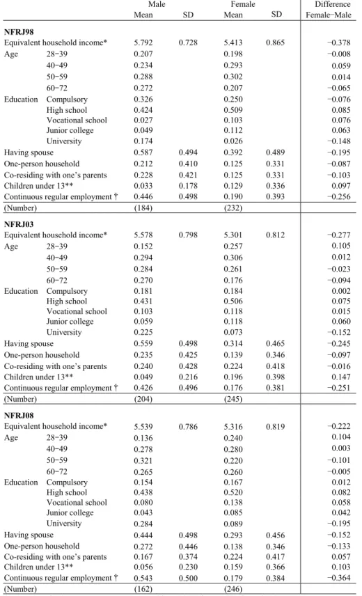
6.2. Gender differences in post-divorce life

Table 6 shows male and female means for the variables used in our analysis. Most variables are two-value coded as 1 or 0 (i.e., so-called “dummy” variables), so that their means equate the proportion of the respondents for whom the condition is satisfied. Cases with missing values are deleted according to list-wise deletion criterion. For this reason, these data include fewer cases than Table 5.

Table 6 shows that the equivalent household income is higher for men and lower for women. This is the same result as seen in Table 5.

7_{The NFRJ08 data include the information (age and co-residence) of the first six living children. The NFRJ98 data include}

information on the age of the first five children (either living or dead) and on co-residence with the first three living children. We used that information to count co-residing young children. We might thereby miss some respondents to be counted as co-residing with their young children, if they have more than six (NFRJ08) or three (NFRJ98) children. For some cases, the respondent was not questioned or did not answered about the co-residence with the child; we counted such a case as a co-residing child, as far as the child was younger than 13 years old.

(10)

Age distribution differs slightly between men and women. The women tend to be younger and the men tend to be older8.

Gender differences are apparent in education. For both men and women, the modal category is high school, but the percentage is greater for women (50–52%) than for men (42–44%). Men show higher percentages of being university graduates (17–28%) than women do (less than 10%). Women show, instead, considerable percentage in the category of junior college (around 10%). Percentage at the compulsory level is almost equal in the NFRJ03 and NFRJ08 data, but slightly higher for men in the NFRJ98 data. On average, you can summarize that men received higher-level education.

Gender differences by family/household conditions are as follows. While the proportion of men who remarried (i.e., those having spouses at the survey date) is 44–59%, for women the proportion is 29–30%. Men thus tend to remarry after divorce at higher likelihood than women. While the proportion of men living alone (in an one-person household) is 21–27%, for women this proportion is around 13%. The percentage is thus higher among men. However, almost no difference is found in the proportions of respondents living with parents for NFRJ03 at around 23%, with the lower figures for women in NFRJ98 (12.5%) and men in NFRJ08 (16.7%). On the other hand, while few men (3–6%) live together with young children, the cases of women doing so are sizable (13–20%).

Gender differences are apparent in employment conditions as well. Around the half of men continued ordinary regular employment, but less than 20% of women have that status.

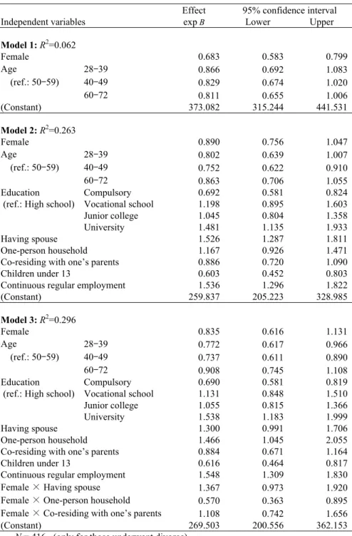
6.3. Regression analysis

We used these variables in multiple linear regression analysis to predict equivalent household income. Although the dependent variable was converted through logarithm transformation, the results appear in Table 7 with estimated coefficients inversely transformed through an exponential function, accompanied with the 95% confidence intervals. We can thus interpret the figures on Table 7 as exhibiting multiplier effects on the equivalent household income. Three models were estimated.

Model 1 checks for the effect of gender, controlling only age composition. The coefficient of the “female" variable is negative for all three surveys. This indicates that women’s equivalent household income tends to be lower in comparison with men’s. The effect was 0.683 for NFRJ98, 0.745 for NFRJ03, and 0.819 for NFRJ08. These values largely correspond to the weighted means of the female/male ratios for the two categories of “Divorced” in Table 5. The value has been rising in this decade, which reflects the narrowing gap between divorced men and women, we have seen.

Model 2 introduces the main effects of the other variables. Education has significant effects by which higher-level education brings about higher income, roughly speaking. The effect of remarriage (=having spouse) is positive. Co-residence with young children has a powerful impact: income would be lowered to 60–70% level by the presence of one’s children under 13 in the household. Other variables concerning household composition — co-residence with parents9_{and one-person household— have no significant effect. Continuous regular}

8_{The gender difference in the age distribution may reflect the tendency toward marriage between an older husband and a younger}

wife. Alternatively, it may be the case that marriages between spouses with greater age differences are more likely to end in divorce. Whichever the case, the data contain a truncation effect in the age of the survey subjects, because they are sampled from the population of people aged 28–72.

9_{Murakami Akane (2009) suggests that divorced women can receive the benefits of living with parents in their own home. Such an}

(11)

employment has a great impact, raising the income by about 50–60%. After controlling for these effects, the variable “female” has no longer significant effect.

Model 3 adds interaction effects between gender and household composition. To easily understand the complex results, we look at Table 8 summarizing the predicted effects based on Model 3 in Table 7. We find the clear effects of interaction for women, with higher income for remarried (=having spouse) women and lower income for women in one-person household. The former has income almost double the latter. In contrast, the effects are not clear for men, with no consistent effect by household composition.

7. Discussion

7.1. Summary of the findings

The results of our analysis provide two interesting sights on the state and causality about economic gender gap in contemporary Japanese society.

First, as we saw in Section 5, the economic disadvantages of women appear among divorced and widowed persons. Unmarried or married (continuing their first marriage) women have no significant disadvantage. This suggests that the growing divorced/widowed population —as a result of marriage instability or of population aging— is the main component of gender inequality. Although divorced/widowed people are still a minority in the Japanese population today, they are nevertheless the key to gender equality.

Second, as we saw in Section 6, there are the four factors with significant effects on equivalent household income after divorce. We confirmed in Table 6 female-male differences in the four factors lowering women’s equivalent household income. We also found in Table 7 that gender has no significant direct effect on equivalent household income, after controlling for the four factors. The causes of the worsening of the standard of living of divorced women can thus be reduced to the following four factors.

Having a low level of education

Not having a continuous career as an ordinary regular employee Co-residing with their young children

Not remarried

These are similar to the results detected by Tanaka (2008). They also offer a quantitative evidence for the hypothesis of marital-life results, because the second and third factors are the very focus of the hypothesis, and they have the strong effect of lowering women’s standard of post-divorce living as derived from the hypothesis.

In addition, as a technical finding, we identify the difference between SSM and NFRJ datasets because of the case selection. As we mentioned in Section 2.2, Tanaka’s (2008) analysis using the SSM2005-J data reported greater gender gap than Tanaka (2010) using the NFRJ03 data. This difference may be due to the fact that remarried people is not included in the analysis by SSM2005-J. The NFRJ03 data in Table 5 show that, among those who divorced but having no spouse, women’s equivalent household income is 66.8% of men’s. This approximately equates the result from SSM2005-J (Tanaka 2008).

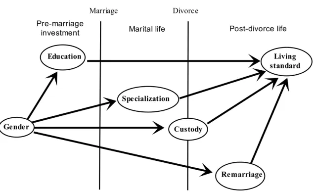
7.2. Gender gap in pre-marriage investment, marital life, and post-divorce life

Now we turn to theoretical perspective on lifecourse and gender gap. Figure 1 illustrates the process of making gender gap in post-divorce life. One’s life is divided into three stages: pre-marriage investment, marital life, and post-divorce life. We map the above-mentioned four factors on these stages.

(12)

The first factor is education as pre-marriage investment. In most cases, people’s school education ends before their marriage, by the early 20s. Once their school education completed, it is difficult to change afterwards. Education is so deeply instituted in the social stratification system that it continues to function as the resource to get the higher standard of living — even after divorce, of course.

The second factor is specialization in marital life. Most couples conduct division of labor, for efficiency in their communal life. This brings about differences in their human capital and social status. Most husbands specialize in paid work and pursue their career as full-time regular employee, without housework burden. In contrast, most wives specialize in housework and give up full-time regular employment to take household responsibilities. As a result, there will be the difference in earning capacity between husbands and wives. A peaceful marital life could conceal the gap, as long as the spouses altruistically support each other10. However, when the marital life is broken, the gender gap will come up to the surface.

The third factor is the assignment of the custody of the couple’s legitimate child. The Civil Code provides that parents can, as far as they are married, take joint custody of their legitimate child. However, once they divorced, the Civil Code does not allow the joint custody; one of the parents should have sole custody. This is instituted in the procedure of divorce, either by mutual consent or by a court decision. In today’s Japan, there is a strong tendency toward the mother becoming the custodial parent after divorce11. Taking custody requires high cost —including children’s living expenses, childcare service charges, educational investment, and opportunity cost due to a career interruption and shorter working hours. This is one of the main causes of gender gap in post-divorce life.

The fourth factor is the probability of remarriage. Results of our analyses have revealed the effect of remarriage enormously improving the living standards for divorced women. Therefore, if women remarried at high probability, it would contribute to lessen the gender gap after divorce. In reality, however, women remarry at lower probability than men do (Table 4 and Table 6). The majority of divorced women remain single after divorce. Hence remarriage does not serve well for gender equalization in post-divorce living standards.

7.3. Against gender gap as a result of marital life

The above results indicate that the family system should bear the primary responsibility for the economic gender gap. Women are disadvantaged after divorce due to the gender gap created through various aspects of the family system. Gender-equal policy should include reformation of the family system to offset such disadvantage.

As discussed in Section 2.2, we already have a proposal for such reformation —toward equity-oriented financial provision on divorce— advocated by family law scholars. They constructed the proposal on the consideration about specialization and children as results of marital life, which overlaps two of the four factors creating women’s post-divorce disadvantage detected in our analysis. On Figure 1, we can think of the area of marital life —between the two vertical lines of “marriage” and “divorce”— as the coverage of the reformation.

10_{Altruism between married couple is normative, rather than voluntary. The Civil Code provides the responsibility of married}

couple to support each other (Article 752) and to share living expenses (Article 760), which is interpreted as providing that husband and wife shall keep the same standard of living between them. This interpretation has its root in the theorization of modern family law by Nakagawa Zen’nosuke (1928), and it has been an accepted legal theory today. However, it is also an accepted theory that such responsibility is terminated by divorce, with a few exceptions of advocators for the idea that the marital responsibility continues permanently, even after divorce. See a review of recent debates by Omura Atsushi (2010) to capture a current overview on those issues.

11_{This has been a recent phenomenon. Before 1960, the majority of custodial parents had been the fathers. Number of the cases of}

custodial mothers grown and exceeded that of fathers in the mid-1960s. Vital Statistics report that, since 2000, the divorced mothers have been the custodial parents at the rate of 80% or more; the fathers at the rate of 20% or less (according to the data compiled by National Institute of Population and Social Security Research (IPSS 2011)).

(13)

Gender gap as a result of the two factors, “specialization” or “custody”, should thus fully be covered12 by financial provision on divorce, to eliminate the gap. Because the two factors exhibit a strong effect in our analysis, we can expect the great contribution by the equity-oriented reformation to promote gender equality, if it is properly carried out.

However, the theoretical possibility aside, we find various obstacles in implementation of equity-oriented reformation. First, divorce has been a largely ignored phenomenon, even in family studies or in gender politics. Today’s reality is far from the establishment of norms that call divorced couples for a full settlement of human capital, social status, and responsibilities for children. Although some progress is being made from a legal perspective, no widespread consensus has been reached on the necessity for such reformation. It is likely to take many years until the equity-oriented principle for divorce law is established and norms are developed that effectively regulate people toward equitable behavior in circumstances of divorce. Second, as a result of the inactiveness in the research about marital-life results on post-divorce life, we have not compiled reliable evidence for decision-making for real divorce cases. There will thus be difficulties to make decision for real cases, even if the equity-oriented principle is accepted (Tanaka 2007a; Tanaka 2007b). Now we have launched on the starting line for the quantitative research of divorce, to uncover the reality of post-divorce life and to predict how law/policy changes effect the gender gap.

References

[Becker 1991] Gary S. Becker. A Treatise on the Family (enlarged edition). Cambridge, MA: Harvard University Press.

[England et al 1990] Paula England, and Barbara S. Kilbourne. “Markets, Marriages, and Other Mates: The Problem of Power”. Roger Friedland, and A. F. Robertson (eds.). Beyond the Marketplace. New York: Aldine de Gruyter.

[Fujiwara 2005] 藤原千沙. “ひとり親の就業と階層性” . 社会政策学会誌.13: 161–75.

[Fukuda 2009] 福田亘孝. “配偶者との別れと再びの出会い: 離別と死別，再婚”. 藤見純子, and 西野理子 (eds.). 現代日本人の家族: NFRJ から見たその姿. Tokyo: 有斐閣. 72–84. [Hamamoto 2005] 濱本知寿香. “母子世帯の生活状況とその施策” . 季刊社会保障研究. 41(2): 96–110. [IPSS 2006] 国立社会保障・人口問題研究所. 少子化の要因としての離婚・再婚の動向、背景および見通しに関する人口学的研究第 1 報告書 (所内研究報告 18). [IPSS 2008] 国立社会保障・人口問題研究所. 少子化の要因としての離婚・再婚の動向、背景および見通しに関する人口学的研究第 2 報告書 (所内研究報告 22). [IPSS 2011] 国立社会保障・人口問題研究所. “表 6-14 親権を行う子をもつ夫妻別離婚数 1950～2009 年” . 人口問題資料集 2011. (Retrieved 2011.7.11, http://www.ipss.go.jp/syoushika/tohkei/Data/ Popular2011/T06-14.xls).

[Iwata 2005] 岩田正美. “政策と貧困”. 岩田正美, and 西澤晃彦 (eds.). 貧困と社会的排除. Kyoto: ミネルヴァ書房.15–41. [Kambara 2006] 神原文子. “母子世帯の多くがなぜ貧困なのか?”. 澤口恵一, and 神原文子 (eds.). 第 2 回家族についての

全国調査 (NFRJ03) 第 2 次報告書 No. 2. Tokyo: 日本家族社会学会全国家族調査委員会. 121–36. [MHW 1999] 厚生省. 人口動態社会経済面調査報告平成 9 年度: 離婚家庭の子ども. Tokyo: 厚生統計協会. [Motozawa 1998] 本沢巳代子. 離婚給付の研究. 一粒社.

12_{Between the remaining two factors, gender difference in the likelihood of remarriage can be covered by financial provision on}

divorce, if it is proved as being resulted from marital life. Theoretically speaking, we can assume the difference as coming from specialization between husband and wife. That is because, in the typical sexual division of labor, the husband accumulates general human capital that can be easily applied outside of the marital relationship, while the wife accumulates specific human capital that is effective only in a particular human relationship, as England et al (1990) summarized. This difference in their human capital can be a source of inequality in the marriage market. If this is the case, we can argue that the difference in the likelihood of remarriage is a result of former marital life. If so, financial provision on divorce should include compensation for such inequality, although such case has not been mentioned in the debate on the reformation of divorce law.

(14)

[Murakami 2009] 村上あかね. “離婚によって女性の生活はどう変化するか?” . 季刊家計経済研究. 84: 36–45. [Nagase 2004] 永瀬伸子. “離別母子家庭の就業と賃金経路”. 社会政策学会第 108 回大会. 2004.5.22, 法政大学. [Nakagawa 1928] 中川善之助. ”親族的扶養義務の本質 (1): 改正案の一批評” . 法学新報. 38(6): 1–22.

[JIL 2003] 日本労働研究機構. 母子世帯の母への就業支援に関する研究 (調査研究報告書 156).

[OECD 2001] Organisation for Economic Co-operation and Development. OECD Employment Outlook, June 2001. [Omura 2010] 大村敦志. 家族法 (第 3 版) . Tokyo: 有斐閣.

[Shinotsuka 1992] 篠塚英子. “母子世帯の貧困をめぐる問題” . 日本経済研究. 22: 77–118. [Suzuki 1992] 鈴木眞次. 離婚給付の決定基準. Tokyo: 弘文堂.

[Tamiya et al 2007] 田宮遊子, and 四方理人. “母子世帯の仕事と育児” . 季刊社会保障研究. 43(3): 219–31.

[Tanaka 2007a] Tanaka Sigeto. “Towards a Lifestyle-Neutral Gender-Equal Policy” (unpublished manuscript). (Retrieved 2008.4.29, http://www.sal.tohoku.ac.jp/~tsigeto/gelapoc/bk12ii5e.html).

[Tanaka 2007b] Tanaka Sigeto. “Against Intra-Household Exploitation”. Paper read at East Asian Social Policy Research Network (EASP), 4th International Conference, 2007.10.20, Tokyo. (http://www.sal.tohoku.ac.jp/~tsigeto/ 07z.html).

[Tanaka 2008] Tanaka Sigeto. “Career, Family, and Economic Risks”. 中井美樹, and 杉野勇 (eds.). 2005 年 SSM 調査シリーズ 9 ライフコース・ライフスタイルから見た社会階層. Sendai: 2005 年 SSM 調査研究会, 21–33.

[Tanaka 2010] Tanaka Sigeto. “The Family and Women’s Economic Disadvantage”. Tsujimura Miyoko, and Osawa Mari (eds.). Gender Equality in Multicultural Societies. Sendai: Tohoku University Press. 215–234.

[Tsuneta et al 1955] 恒田文次, 吉村弘義, 村崎満, 大浜英子, 塩田サキノ, and 小林麗子. “離婚の慰藉料と財産分与” (round table). 法律のひろば. 8(5): 26–35.

[Wagatsuma 1953] 我妻栄. 改正親族・相続法解説 (12 刷). Tokyo: 日本評論新社.

Acknowledgement

The data for this secondary analysis, National Family Research of Japan 1998 (NFRJ98) and National Family Research of Japan 2003 (NFRJ03) by the NFRJ Committee, Japan Society of Family Sociology, was provided by the Social Science Japan Data Archive, Information Center for Social Science Research on Japan, Institute of Social Science, The University of Tokyo. The author also gratefully acknowledges the permission for the use of the National Family Research of Japan 2008 (NFRJ08) data by the NFRJ Committee, Japan Society of Family Sociology.

The earlier versions of this paper were presented at the internal conferences of “NFRJ08 研究会” [the joint-use project of the NFRJ08 data closed to the members of the Japan Society of Family Sociology] (in Tokyo, 2010.7.3, 2010.12.24, and 2011.7.24) and are to be compiled by September 2011 as a chapter of the report of the project. Presentations were also made at the 20th annual meeting of the Japan Society of Family Sociology (in Tokyo, 2010.9.3) and at the 23rd monthly seminar of the Global COE Program of Tohoku University (in Sendai, 2011.2.16). The author gratefully thanks the comments from the audiences and the financial support from the Global COE Program of Tohoku University.

Address of the author

TANAKA Sigeto (田中重人) < http://www.sal.tohoku.ac.jp/~tsigeto/>

Applied Japanese Linguistics, Faculty of Arts and Letters, Tohoku University (東北大学文学部日本語教育学専修) Kawauti 27-1, Aoba Ku, Sendai Si, Miyagi Ken (宮城県仙台市青葉区川内 27-1)

(15)

Table 2. Synopsis of NFRJ surveys

(A) About All NFRJ surveys (NFRJ98, NFRJ03, NFRJ08)

Survey name 全国家族調査 (National Family Research of Japan)

Survey organizer 日本家族社会学会全国家族調査委員会(Japan Society of Family Sociology, NFRJ Committee)

Survey company 社団法人中央調査社 (Central Research Service Inc.)

Survey area All over Japan

Sampling method Stratified two-stage probability sampling

Survey method Self-administered questionnaire, home delivery, leave and pick-up

Website http://www.wdc-jp.com/jsfs/english/nfrj.html

(B) The first survey (NFRJ98)

Population Japanese nationals living in Japan and born between 1921 and 1970 (28 to 77 years old as of the end of 1998)

Sample size 10,500 (response 6,985; response rate 66.5%)

Survey period January to February 1999

Data availability Deposited at the SSJ Data Archive by the University of Tokyo (Survey Number 0191)

Data used in this paper From SSJ Data Archive, downloaded 2010.6.4

We use only respondents aged 28–72 in this paper, to keep comparability with NFRJ08.

(C) The second survey (NFRJ03)

Data availability Deposited at the SSJ Data Archive by the University of Tokyo (Survey Number 0517)

Data used in this paper From SSJ Data Archive, downloaded 2010.6.4

We use only respondents aged 28–72 in this paper, to keep comparability with NFRJ08.

(D) The third survey (NFRJ08)

Data availability Close to the members of Japan Society of Family Sociology until summer 2011

Data used in this paper Version 4.0 (2011.2.18 distribution)

Table 1. Trends in the composition of marital status in population of 25–69 years old, 1960–2005

Male Female Year

Unmarried Married Widow Divorced Total (Number) Unmarried Married Widow Divorced Total (Number)

1960 11.7 84.1 3.0 1.2 100.0 (21,593,336) 7.2 75.6 14.3 2.9 100.0 (23,275,570) 1965 11.3 85.3 2.4 1.0 100.0 (24,114,635) 6.9 77.6 12.8 2.6 100.0 (25,807,568) 1970 11.4 85.6 1.8 1.1 100.0 (26,701,456) 6.6 79.1 11.6 2.8 100.0 (28,523,108) 1975 12.9 84.4 1.5 1.2 100.0 (30,233,046) 7.4 79.9 10.1 2.6 100.0 (31,986,738) 1980 14.0 83.2 1.3 1.5 100.0 (32,448,710) 7.5 80.7 8.8 3.0 100.0 (34,127,260) 1985 15.3 81.3 1.3 2.1 100.0 (33,996,126) 8.2 80.2 7.8 3.8 100.0 (35,444,839) 1990 17.2 79.0 1.4 2.4 100.0 (35,367,436) 9.8 79.2 6.9 4.1 100.0 (36,474,317) 1995 19.9 75.8 1.4 2.9 100.0 (37,036,122) 12.0 77.0 6.3 4.7 100.0 (37,662,753) 2000 23.1 72.1 1.4 3.4 100.0 (38,034,663) 14.7 74.1 5.7 5.5 100.0 (38,656,441) 2005 25.6 69.0 1.3 4.2 100.0 (37,895,517) 16.6 71.7 5.0 6.6 100.0 (38,574,018)

Excluding the unanswered cases. Calculated from Population Census (国勢調査), time series data, Table 4 “配偶関係 (4 区分),年齢 (5 歳階級), 男女別 15 歳以上人口: 全国 (大正 9 年～平成 17 年)” (da04.xls). Downloaded from “政府統計の総合窓口” (Portal Site of Official Statistics of Japan, http://www.e-stat.go.jp/, 2011.2.7).

(16)

Table 4. Distribution of marital history

Widowed Divorced Survey Gender Continued

1st marriage with spouse no spouse with spouse no spouse Unmarried Total (N) NFRJ98 Male 80.0 0.5 1.8 3.5 2.7 11.5 100.0 (3128) Female 77.6 0.3 6.9 2.9 4.6 7.7 100.0 (3399) V=0.147 Total 78.8 0.4 4.5 3.2 3.6 9.5 100.0 (6527) NFRJ03 Male 78.1 0.6 2.3 4.1 3.6 11.3 100.0 (2819) Female 77.5 0.3 6.7 2.7 5.6 7.2 100.0 (3148) V=0.137 Total 77.8 0.4 4.6 3.4 4.6 9.2 100.0 (5967) NFRJ08 Male 75.6 0.4 1.8 3.2 4.2 14.8 100.0 (2441) Female 74.0 0.3 5.4 3.0 7.3 10.0 100.0 (2743) V=0.132 Total 74.8 0.3 3.7 3.1 5.9 12.3 100.0 (5184)

V: Cramer’s coefficient of association (p < 0.01 for all). Those who were both divorced and widowed were categorized into “Divorced”.

Table 3. Gender and equivalent household income (geometric mean in 10,000 yen)

Male Female Total Female/Male Missing

NFRJ98 Geometric mean 352.1 315.8 333.3 0.897 R2_{=0.006 (Number)} ₍₂₉₂₈₎ ₍₂₉₈₉₎ ₍₅₉₁₇₎ ₍₆₁₀₎ NFRJ03 Geometric mean 304.3 281.5 292.1 0.925 R2_{=0.003 (Number)} ₍₂₆₀₃₎ ₍₂₈₇₈₎ ₍₅₄₈₁₎ ₍₄₈₈₎ NFRJ08 Geometric mean 308.8 287.7 297.5 0.932 R2_{=0.003 (Number)} ₍₂₁₆₅₎ ₍₂₃₉₄₎ ₍₄₅₅₉₎ ₍₆₃₀₎

Table 5. Gender, marital history, and equivalent household income (geometric mean in 10,000 yen)

Survey Marital History Male Female Female/Male

G. Mean N G. Mean N Ratio

NFRJ98 Continued 1st marriage 358.0 (2363) 342.5 (2337) 0.957

R2

=0.047 Widowed, but with spouse 461.3 (14) 374.5 (6) 0.812

Widowed, no spouse 250.6 (54) 203.8 (202) 0.814

Divorced, but with spouse 338.5 (108) 315.8 (94) 0.933

Divorced, no spouse 312.5 (76) 178.8 (142) 0.572

Unmarried 339.4 (313) 284.9 (208) 0.840

R2

=0.040 Widowed, but with spouse 369.6 (15) 172.7 (9) 0.467

Unmarried 279.5 (285) 280.6 (192) 1.004

R2_{=0.057 Widowed, but with spouse} _496.9 ₍₈₎ _339.9 ₍₆₎ _0.684

Unmarried 279.2 (311) 279.0 (240) 0.999

Results of ANOVA: p<0.05 for all of the main and interaction effects (by Type III SS). Classification of marital history is the same as Table 4.

(17)

Table 6. Descriptive statistics for regression analysis (only those who underwent divorce)

Male Female Difference

Mean SD Mean SD Female−Male

NFRJ98

Equivalent household income* 5.792 0.728 5.413 0.865 −0.378

Age 28–39 0.207 0.198 −0.008 40–49 0.234 0.293 0.059 50–59 0.288 0.302 0.014 60–72 0.272 0.207 −0.065 Education Compulsory 0.326 0.250 −0.076 High school 0.424 0.509 0.085 Vocational school 0.027 0.103 0.076 Junior college 0.049 0.112 0.063 University 0.174 0.026 −0.148 Having spouse 0.587 0.494 0.392 0.489 −0.195 One-person household 0.212 0.410 0.125 0.331 −0.087

Co-residing with one’s parents 0.228 0.421 0.125 0.331 −0.103

Children under 13** 0.033 0.178 0.129 0.336 0.097

Continuous regular employment† 0.446 0.498 0.190 0.393 −0.256

(Number) (184) (232)

NFRJ03

Age 28–39 0.152 0.257 0.105 40–49 0.294 0.306 0.012 50–59 0.284 0.261 −0.023 60–72 0.270 0.176 −0.094 Education Compulsory 0.181 0.184 0.002 High school 0.431 0.506 0.075 Vocational school 0.103 0.118 0.015 Junior college 0.059 0.118 0.060 University 0.225 0.073 −0.152 Having spouse 0.559 0.498 0.314 0.465 −0.245 One-person household 0.235 0.425 0.139 0.346 −0.097

Co-residing with one’s parents 0.240 0.428 0.224 0.418 −0.016

Children under 13** 0.049 0.216 0.196 0.398 0.147

(Number) (204) (245)

NFRJ08

Age 28–39 0.136 0.240 0.104 40–49 0.278 0.280 0.003 50–59 0.321 0.220 −0.101 60–72 0.265 0.260 −0.005 Education Compulsory 0.154 0.167 0.012 High school 0.438 0.520 0.082 Vocational school 0.080 0.138 0.058 Junior college 0.043 0.085 0.042 University 0.284 0.089 −0.195 Having spouse 0.444 0.498 0.293 0.456 −0.152 One-person household 0.272 0.446 0.138 0.346 −0.133

Co-residing with one’s parents 0.167 0.374 0.224 0.417 0.057

Children under 13** 0.056 0.230 0.159 0.366 0.103

(Number) (162) (246)

Mean: arithmetic mean. SD: standard deviation. *: Natural logarithm of equivalent household income in 10,000 yen. **: For those who had spouse, children were counted only when their age was greater than the duration since the remarriage.

†: Those who had no experience of quitting their job because of childbirth or similar reasons, and were ordinary regular employees (常時雇用されている一般従業者) at the survey date.

Categories for education: Compulsory (中学校); High school (高等学校, including miscellaneous category); Vocational school (専門学校, after graduation of high school); Junior college (短期大学, in two years, and 高等専門学校=technical collage); University (大学, in four years or more, and graduate school)

(18)

Table 7. Regression analysis of equivalent household income (in 10,000 yen)

(A) NFRJ98

Effect 95% confidence interval

Independent variables exp B Lower Upper

Model 1: R2_=0.062 Female 0.683 0.583 0.799 Age 28–39 0.866 0.692 1.083 (ref.: 50–59) 40–49 0.829 0.674 1.020 60–72 0.811 0.655 1.006 (Constant) 373.082 315.244 441.531 Model 2: R2_=0.263 Female 0.890 0.756 1.047 Age 28–39 0.802 0.639 1.007 (ref.: 50–59) 40–49 0.752 0.622 0.910 60–72 0.863 0.706 1.055 Education Compulsory 0.692 0.581 0.824

(ref.: High school) Vocational school 1.198 0.895 1.603

Junior college 1.045 0.804 1.358

University 1.481 1.135 1.933

Having spouse 1.526 1.287 1.811

One-person household 1.167 0.926 1.471

Co-residing with one’s parents 0.886 0.720 1.090

Children under 13 0.603 0.452 0.803

Continuous regular employment 1.536 1.296 1.822

(Constant) 259.837 205.223 328.985 Model 3: R2_=0.296 Female 0.835 0.616 1.131 Age 28–39 0.772 0.617 0.966 (ref.: 50–59) 40–49 0.737 0.611 0.890 60–72 0.908 0.745 1.108 Education Compulsory 0.690 0.581 0.819

University 1.538 1.183 1.999

Having spouse 1.300 0.991 1.706

Children under 13 0.616 0.464 0.817

Female × Having spouse 1.367 0.973 1.920

Female × One-person household 0.570 0.363 0.895

Female × Co-residing with one’s parents 1.108 0.742 1.656

(Constant) 269.503 200.556 362.153

N = 416 (only for those underwent divorce)

(19)

Table 7. Regression analysis of equivalent household income (in 10,000 yen) [continued]

(B) NFRJ03

Effect 95% confidence interval Independent variables exp B Lower Upper

(ref.: High school) Vocational school 1.199 0.957 1.504 Junior college 1.120 0.877 1.430

University 1.633 1.323 2.014

Having spouse 1.307 1.092 1.565

Children under 13 0.669 0.528 0.848

(ref.: High school) Vocational school 1.160 0.928 1.450 Junior college 1.097 0.862 1.396

University 1.652 1.344 2.031

Having spouse 0.908 0.675 1.221

Children under 13 0.703 0.556 0.890

Female × One-person household 0.996 0.632 1.570 Female × Co-residing with one’s parents 1.068 0.734 1.553

(Constant) 250.015 181.293 344.787

N = 449 (only for those underwent divorce)

(20)

Table 7. Regression analysis of equivalent household income (in 10,000 yen) [continued]

(C) NFRJ08

Effect 95% confidence interval Independent variables exp B Lower Upper

University 1.385 1.132 1.694

Having spouse 1.384 1.147 1.671

Children under 13 0.601 0.470 0.768

University 1.387 1.134 1.696

Having spouse 1.284 0.904 1.824

Children under 13 0.601 0.470 0.768

Female × One-person household 0.707 0.447 1.119 Female × Co-residing with one’s parents 0.891 0.556 1.427

(Constant) 157.728 112.927 220.302

(21)

Table 8. Effects of gender, remarriage, and household composition

Female Male Having

spouse One-person household

Co-residing with

one’s parents Having spouse One-person household

Co-residing with one’s parents

NFRJ98 1.483 0.697 0.818 1.300 1.466 0.884 NFRJ03 1.276 0.592 0.702 0.908 0.803 0.888 NFRJ08 1.750 0.971 1.264 1.284 1.191 1.230

Calculated based on the estimated effects for the Model 3 on Table 7.

The baseline (=0) is men who have no spouse, are not in one-person household, and are not co-residing with one’s parents.

Gender Education Custody Specialization Remarriage Living standard Marriage Divorce Post-divorce life Marital life Pre-marriage investment