C25 1995 5 VTS 最近の更新履歴 Hideo Fujiwara

A Scheduling Problem in Test Generation

Abstract

Tomoo Inoue, Hironori Maeda and Hideo Fujiwara

Graduate School of Information Science

Nara Institute of Science and Technology

89 16-5, Takayama, Ikoma, Nara 630-O 1, Japan

The order of faults which are targeted for test- analyze the effect of scheduling based on test-pattern pattern generation affects both of the processing time for test generation time and dominclting prohabili~. Finally, we generation and the number of test-patterns. This order is present experimental results on the ISCAS’85 [8] benchmark referred to as a test generation shedule. In this paper, we circuits.

consider the test generation scheduling problem which

minimizes the cost of testing. We analyze the effect of 2. Formulation of the Scheduling Problem

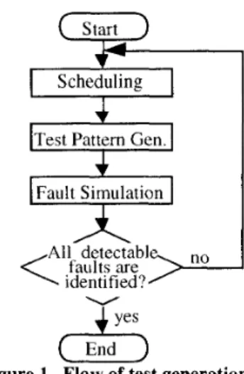
scheduling based on test-pattern generation time and The flow of our test generation process is illustrated domincrting probability. Then, we present experimental in Figure 1. Let F be a set of faults of a given results on the ISCAS’85 benchmark circuits. combinational circuit. Let A be a test-pattern generation

algorithm in this process. 1. Introduction

The cost of testing for logic circuits consists mainly of the cost of test generation and the cost of test application. The cost of test generation means the processing time to generate test-patterns for a given circuit. Several efficient test generation algorithms such as PODEM [I], FAN [2] and SOCRATES [3] are reported for combinational circuits. On the other hand, small test set is important for the reduction of the cost of test application. By applying test compaction algorithms as reported in [4-71 to test generation, small test

First, Test Genercrtion Scheduler makes a test generation schedule S for fault set F, i.e., determines an order of target faults in fault set F to be test-generated. Test- Pattern Generator generates a completely-specified test- pattern for the target fault selected according to schedule S, by algorithm A. Fault Simulator identifies all the faults that are detected by the test-pattern. Test-pattern generation and fault simulation are both repeated until all detectable faults in F are identified. In this process the number of test- patterns and the processing time for test generation depend sets can be obtained. However, since test compaction on schedule S as well as on test-pattern generation algorithm approaches require extra efforts such as deriving maximal A. Hence, we can consider two optimal scheduling independent fault sets, the total cost of testing is not always problems; one is to minimize the test generation time, and

reduced. the other is to minimize the number of test-patterns for fault

Many test generation algorithms consist of two set F with algorithm A

processes; test-pattern generation and fault simulation. In However, to simplify the analysis, we focus only on the test-pattern generation process, a fault is selected from a the processing time for test-pattern generation (denoted by jkdt list, referred to as a target,fiudt, and a test-pattern is TPG time) and the number of generated test-patterns generated for the fault. Then all the detectable faults by the hereafter. Let TA(S) be the total TPG time by schedules test-pattern are identified in fault simulation process. These with algorithm A. Let LA(S) be the total number of test- two processes are repeated until all detectable faults are patterns by schedule S with algorithm A. One of the identified. Here, the order of target faults selected from the optimal scheduling problems is to find an optimal fault list is referred to as the test gene&on sclzdule. The scheduling STopt which minimizes the total TPG time for test generation schedule affects both the processing time for fault set F with algorithm A :

test generation and the test set size (the number of test- patterns), and accordingly there exists an optimal schedule

TA( ‘Top,) = m;n { TA(s)} which minimizes the test generation time and/or the test set

size.

and the other is to find an optimal scheduling SLopt which minimizes the total number of test-patterns for fault set F In this paper, we consider this scheduling problem in with algorithm A :

test generation for combinational logic circuits. First, we LA(SZ>o~r) = min {LA(s)} formulate the scheduling problem, and propose a relation ^S

calledfimlt dnminnnce to estimate the test-pattern generation Note that test-patterns generated by algorithm A are time and the number of generated test-patterns. Then, we completely-specified, i.e., generated test-patterns by

1995 IEEE VLSI Test Symposium, pp. 344-349, May 1995.

Scheduling 4 Test Pattern Gen.

4 Fault Simulation

Figure 1. Flow of test generation algorithm A include no don’t-care value. definefLAt dominance as follows

Hence, we can

Fault Dominance: If the test-pattern for a fault fi generated under an algorithm A detects another fault ,f;, then faultj) domincltes faultjj under algorithm A.

Unless otherwise noted, from now on we will omit the notation of algorithm A for simplicity.

Next we shall consider the probability that a test-pattern for a fault is generated. Let N be the total number of faults. Suppose that a test generation schedule s=<f, ,f;, . ,&. Let “ij be the probability that faultfi dominates faultji. Let Ki be’the probability that a test-pattern for the i-th faultf; in schedule S is generated. Then, the probability that a test- pattern for the first faultfl is 1, i.e., g1 = 1. The second fault f2 is dominated by fl in probability d12. The probability that a test-pattern for f2 is generated is the probability thatJi is not dominated byfl. Hence, g2 = (1 - d12). Similarly, fl andf2 dominate the third fault & in proba.bility d13 and in probability ~$3, respectively. The probability that a test-pattern for fault

f3

is generated is the probability that

f3

is dominated neither by f‘l nor by f2 for which a test-pattern is generated in probability g2. Hence g3 = ‘( 1 - d13) (1 - g2dZ3). In this way, we can express the probability that a test-pattern for the i-th fault is generated can be expressed as

i x1= 1

i- 1

Ri= I-I (l-m&k;) (2 5 i s N)

k= I (1)

Note that the probability dij that fault ,~i dominates fault $ depends on the dominated fault fj, i.e., dq # 4k if j # k in general. However, here we consider the case that the probability is independent of any dominated fault, i.e., dij =

di for all j, and define the dominuting ,prohability as follows. Dominating probability: Let the dominating probability di of a faultfi be the average of the probabilities

dij for allj, i.e.,

By substituting dk for dkj in Equation (l), we have

i g1=1

i- 1

\

gi= I-Jr (l-g&) k=l

= gi-1 (’ -g&l diml) (2 s i s N)

₍₂₎

Note that if 0 < ~ij I 1, then

gi>Xi+l forl<i<N-1. (3)

The total number of test-pattenns obtained by schedule S is 4-Y = 2 I:i

s (4)

and the total TPG time by schedule S is T(S) = 2 ljgi

s (5)

Therefore, if we can predict fault characteristics such as dominating probability and TPG time for each fault CI priori, we can estimate both of the: total number of test-

patterns and the total TPG time obtained by test generation scheduling based on these c:haracteristics. ‘In the next section, we shall analyze the effect of the test generation scheduling based on dominating probability and TPG time provided that these two characteristics are given a priori. 3. Analysis of the Effect of Scheduling 3.1 Scheduling Based on TPG Time

First, we consider a scheduling based on the TPG time for each fault. Here we assume that dominating probabilities for all faultsfi ;are equal, i.e., 4 = d Then, from Equation (2), the probability I;li that a test-pattern for the i-th fault

fj

is generated can be expressed as:

i g1=1

gi = tzi-1 (1 -gi-1 (I) (2 5 i s N)

Let Sh be a schedule or an order of hults. Let

ti

be the TPG time for the i-th fault in order Sh. Suppose an arbitrary pair of adjacent faults (/,,

fn+ 1

) in order 2ih such that

tn

>

tn+

1. Notethat 1 <nIN-1. Let

th=tn

andt,=t,+l. Letgi be the probability that a test-pattern for the i-th fault in order Sh is generated. From Equation (4) lthe total number of test- patterns obtained b:y schedule :?,, is g,iven by

y”/L) = ” gi

h 3

From Equation (5) the total TPG time is given by 7(sh) = c f&?i

S/L .

(6)

Let Se be the order obtained by exchanging the n-th and the (n+l)-th faults in order Sh. Let

tlj

be the TPG time for the i- th fault in order S,. That is,

i

t;, = t,, t;,+1 = t/, i =

ti

(i#n,n+ 1)

(7) Let gli be the probability that a test-pattern for the i-th fault in order S, is generated. From Equation (4) the total number of test-patterns obtained by schedule Se is given by

yq = x RI se

From Equation (5) the,total TPG time is given by qse) = If tigi

s, .

Since 4 = d for all i , Ri = g’j for all i. _Hence, yq = 451) .

(8)

From this equation we can easily see that any scheduling based on TPG time derives the same number of test-patterns provided that dominating probabilities for all faults are Npl.

From Equations (6), (7) and (8), the difference between these two total TPG time can be expressed as

q&L) - q?) = (92 -q (&-&r+l)

Since

th

>

te

and g, > g,+ 1 (from Inequality (3)),

T(?L) - 7(h) > O

This inequality means that when the TPG time for a fault is larger than that for the next fault in an order or a test generation schedule, the total TPG time can be reduced by exchanging these two faults. Hence, the ascending order of TPG time can be obtained by repeating this exchange until no exchange can be applied, and this order minimizes TPG time. Therefore, we have the following theorem.

Theorem I: The scheduling according to the ascending order of TPG time minimizes the total TPG time provided that dominating probabilities for all faults are equal. 3.2 Scheduling Based on Dominating Probability

Next, we consider a scheduling based on dominating probability of each fault. Here we assume that TPG times for all faultsfj are equal, i.e.,

ti

=

t.

Then, from Equations (4) and (5) the total TPG time by a schedule S can be expressed as

7(S) = 2

tg;

= t I!.(S) s

Let S bf

be an order of faults. Let 4 be the dominating proba ility of the i-th fault in order SY Suppose an arbitrary pair of adjacent faults f,, fntl m

n+l. Notethatl<n<N-1.)Let d

order Sf such that d, < 9 =dn andd, =dn+L. Let gi be the probability that a test-pattern for the i-th fault in order Sf is generated. From Equation (2) we have

g,,+1 = g,/ (’ -SI? df) ) ₍₉₎ and

8,,+2 =gn+1 (1 -Rn+1 d,,) .

Thus the total number of test-patterns generated in order Sf can be expressed from Equation (4) as

ysj = 2 gi

9 . ⁽¹⁰⁾

Let S, be the order obtained by exchanging the n-th and the (n+l)-th faults in order St Let di be the dominating probability of the i-th fault in order Sm. That is,

i

4, = 4P d+l = df dj = di (i#n,n+ 1)

(‘1) Let g’i be the probability that a test-pattern for the i-th fault in order S, is generated. From Equation (2) we have

i,+I = g;, ( 1 - iL %) )

₍₁₂₎

and

g/1+2 = gn+ 1 (1 -i,+1 dj) .

Thus the total number of test-patterns generated in order S, can be expressed from Equation (4) as

4%l)

^{= 2 RI}

s m (13)

From Equations (10) and (13) the difference between L(Sf) and L(S,) can be expressed as

4sf))-4sin)

= iii (fii-fij;) + (fin+1 -gl+l) i= 1

+ ( Bllf? ^{- sn+?:} ’ ^{)+ : ($4)}

i = n+3

Since pi = d ‘i for i 5 n - 1 (Equation (1 1)), from Equation (2) we have

gi ‘g’i for i 5 ?I. ₍₁₄₎

Hence,

~ (gi-g~)=O i= 1

From Equations (9), (12) and (14) and 9 < dm, we have g//+1 -RI,+1 =R~(d,,,-djj>O .

In the same way as the above inequality we have

gt,+2 - i,+? = 4 df 4, pm - df) ’ 0 . ₍₁₅₎

On the other hand, the difference between the probability that a test-pattern for the i-th fault is generated in order Sf and that in order S, can be expressed from Equation (2) as

,j-81=(~tl-R11)(1-(gC1+S~-l)di-l) .

₍₁₆₎

If we assume that 4 < l/2 for all i, which is reasonable, then we have

K;-1 + KJ-1 < 1 ₍₁₇₎

in IEquation (16). Hence, from Equation (16) and Inequalities (15) and (171, we have

gj-1 - s;-1’ 0 for n + 3 I i I N. Therefore,

i! (fii-fii)>O i = 11+3 Thus we have

yqpq%~)~” ) and ;accordingly

(1%

T(q - T(%,) > O ₍₁₉₎

Inequalities (18) and (19) mean that when the dominating probability of a fault is smaller than that of the next fault in an order, the total TPG time as well as the total number of test-patterns can be reduced by exchanging these two faults. Hence, the descending order of dominating probability can be obtained by repeating this exchange until no exchange can be applied, and this order minimizes both of the total TPG time and the total number of test-patterns. Therefore, we have the following theorem.

Theorem 2: The scheduling according to the descending order of dominating probability minimizes both of the total TPG time and the total number of test-patterns provided that TPG times for all faults are equal.

3.3 Scheduling Based on TPG Time

and Dominating Probability

Until now, we considered a scheduling based on either TPG time or dominating probability. Here we consider a scheduling based on both of TPG time and dominating probability.

Let S, be an order of faults. Let 4 be the dominating probability of the i-th fault in order S,. Let ‘i be the TPG time for the i-th fault in order S, Suppose an arbitrary pair of adjacent faults (fn, .fn+ 1) in order S, such that d, > dn+ 1. Note that 1 I n 5 N - 1. Let gi be the probability that a test-pattern for the i-th fault in order S, is generated.

Let Sb be the order obtained by exchanging the n-th and the i:n+l)-th faults in order S, Let d ‘i be the dominating probability of the i-th fault in order Sb. Let f’i be the TPG

time for the i-th fault in order Sb. That is,

i

4, = 4, 1) 4, ‘= h+ 13 4+1 = 4, i+ 1 = 4, d,: = do tl= ti (i # n, n -k 1)

(20)

Let R’i be the probability that a test-pattern for the i-th fault in order Sh is generated

First, let us consider the total number of test-patterns. From Equation (4) we have

4s~)~ lil gi 7 Z-fSb)= ;T: gj. iz= 1

In the same way as the analysis in the previous subsection 3.2, we have g; =g’i for i I n , gi < g’i for n I i 5 N. Hence, the difference between the total number of test- patterns by order S and that Iby order Sb is expressed as

qq-&)<O

In this way, the total number of test-patterns is derived only from the dominating probabilities of all faults independently of TPG time for any fault. Therefore, we have the following theorem.

Theorem 3: The scheduling according to the descending order of dominating probability minimizes the total number of test-patterns.

Next, let us consider the total TPG time. From Equation (5) we have

qs,)= j, rjgj , T&J= $ t;g;. i=l From Equation (2) we have

g,i+1 = >:n (1 - g, d/l) .

Since gi = g’i for i I n , from Equation (20) we have RJt+ 1 = 1::2 (1 - iI d;)

= $:I? (l - gn &+l) .

Thus the difference between the total TPG time by order S, and that by order Sb is

(21)

Since gi < g’i Born 5 i I N, ^we: have

ii li[~j-R))<” i = it+3

Hence, if

t _4,

LL+--

t t1+l ‘&+I > then

Therefore, we have the following theorem.

Theorem 4: The scheduling according to the descending order of dominating probability minimizes the total TPG time provided that

ti di -S--

‘.i ti

for any pair of faults u;,jj) such that di > L$ and

ti

> 5 As shown by Theorem 4, the total TPG time is not always minimized by the scheduling according to the descending order of dominating probability. However. since 4 ’ dn+l in Equation (21), if I, 5 fn+l, then

7&)- T(Sb)<O

Further, as shown by Theorem 3, the total number of test- patterns is always minimized by the scheduling according to the descending order of dominating probability. Hence, we can consider that the scheduling according to the descending order of dominating probability prior to the ascending order of TPG time for each fault would be effective in reducing both of the total TPG time and the total number of test- patterns.

4. Experimental Results

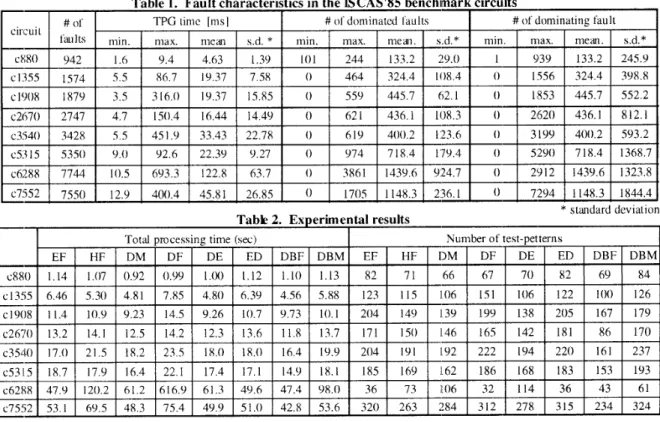
We made experiments of test generation scheduling based on TPG time and dominating probability using the ISCAS’85 benchmark circuits [8] on a DECstation 5000/25. The FAN algorithm [2] was used as a test-pattern generator. In order to obtain accurate fault characteristics for test generation such as TPG time and dominating probability, we computed the CPU time of test-pattern generation for each fault and the number of faults dominated by each fault on the benchmark circuits by using FAN. Note that the number of faults dominated by a fault over the total number of faults denotes the dominating probability of the fault in the above- mentioned analysis. Table 1 shows the computational results for the benchmark circuits.

Based on the above computed characteristics of faults, the following test generation schedules were implemented. (EF) Ascending order of CPU time, called an Ea.sx Fault

first scheduling.

(HF) Descending order of CPU time, called a Hard Fcultfir.\t scheduling.

(DM)Descending order of the number of dominated faults, called a Dominating-Many fklt,fir.st scheduling.

(DF) Ascending order of the number of dominated faults. called a Dominating-Few felt first scheduling.

(DE) DM prior to EF: DM is applied first. For the faults that tie in DM, i.e., dominate the same number of faults. EF is applied.

(ED) EF prior to DM: EF is applied first. For the faults that tie in EF, i.e., require the same CPU time, DM is

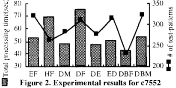
Table 2 and Figure 2 show the total processing time (including fault simulation time) and the number of generated test-patterns for each scheduling method. From these results we can see that the EF and DM schedulings can reduce the total processing time for the most circuits compared with the HF and DF schedulings, that both the total processing time and the number of test-patterns by the DM scheduling are smaller than those by the DF scheduling for all the circuits except ~6288. These results coincide with our analytical results. On the other hand, we can see that the total number of test-patterns by the EF scheduling is larger than that by the HF scheduling for all the circuits except ~6288. This is because dominating probability might not be independent of TPG time. The experimental result for ~6288 is exceptional. In ~6288 dominating-many faults might be easy-to-test, and faults dominated by dominating- many faults would overlap one another. Further, dominating- few faults might be hard-to-test, and faults dominated by dominating-few faults would be different from one another. In this way, the scheduling based only on the dominating probability is not effective for such circuits as ~6288.

In the previous section, we considered the dominating probability. which is the probability that a faults dominates other faults. On the other hand, we can also consider the dominrltedprohahili~ which refers to the probability that a fault is dominated by the other faults. Note that the dominated probability of a fault pi is given by the number of faults that dominate fault j; over the total number of faults. We computed the number of faults that dominate a fault for each fault by using FAN. Table 1 shows the computational results for the benchmark circuits. In Table 1. the number of faults that dominate a fault is denoted by the number of dominating faults.

Table 2 and figure 2 show the experimental results of the scheduling based on the number of dominating faults. DBF means the scheduling according to the ascending order of the number of dominating faults, which is called the Dominclted-Bx-Fewfbult first scheduling, and DBM means the scheduling according to the descending order of the number of dominating faults, which is called the Dominated- B>.-Many frrult first scheduling. From these results we can see that both the total CPU time and the total number of

EF HF DM DF DE EDDBFDBM -

Figure 2. Experimental results for ~7552

test-patterns by the DBF scheduling are smaller than those pattern generation algorithms,” IEEE Trclns. Comyut., by the DBM scheduling for all circuits without exception. vol. C-32, No.12, pp. 1137-1144, Dec. 1983.

Furthermore, we can see that the DBF scheduling is the [3] M. H. Schulz and E. Auth, “Improved deterministic test most effective to reduce both of the total CPU time and the pattern generation with applications to redundancy total number of test-patterns simultaneously for all circuits identification,” IEEE Trans. Computer-Aided Design, vol. of all the schedulings. This is because the standard deviation 8, No. 7, pp. 8111-816, July 1989.

of the number of dominating faults is large as compared [4] S. B. Akers and C. Joseph, “On the role of independent with that of the number of dominated faults for all circuits. fault sets in the generation of minimal test sets,” Proc.

5. Conclusions and Future Work

Int. Test Conf., pp. 1100-l 107, 1987.

In this paper, we considered a scheduling problem in [5] I. Pomeranz, L. N. Reddy and S. M. Reddy, test generation for combinational logic circuits. We analyzed “COMPACTEST: A method to generate compact test sets the effect of the scheduling based on dominating prohahili~ for combinational circuits,” Proc. Int. Test Cnnj:, pp.

194-203, 1991. and test-pattern genercrtion time for each fault, and presented

experimental results on ISCAS’85 benchmark circuits. Ana- [6] G. J. Tromp, “Minimal test sets for combinational

lytical and experhetltd ESldtS show that the schedulings circuits,” Proc. Int. Test Co@, pp. 204-209, 1991.

based on test-pattern generation time, dominating

[71 S, ^Kajihara, 1. ~~~~~~~~~ K, Kinoshita, and S,M. R@, probability and dominated probability are effective in “Cost-effective generation of minimal test sets for stuck-at reducing the cost of testing. One of the remaining problems faults in combinational logic circuits,” Proc. 30th ACM/ is how to obtain these measures without consuming much IEEE Design Automation Conf:, pp. 102-106, 1993. time before test-pattern generation. [8] F. Brglez and H. Fujiwara, “A neutral netlist of ten

combinational benchmark circuits and a target translator in

References

^FORTRAN,” Proc. IEEE Int. Symp. Circuits and

[l] P. Goel, “An implicit enumeration algorithm to generate Systems, June 1985.

tests for combinational logic circuits,” IEEE Trans. [9] P. Agrawal, V.D. Agrawal and Joan Vlloldo, “Test Comput., vol. C-30, No.3, pp. 215222, Mar. 1981. pattern generation for sequential circuits on a network of [2] H. Fujiwara and T. Shimono, “On the acceleration of test workstations,” Proc. 2nd Int. Symp. High Perjhmance

Distributed Computing, pp. 114- 1:20, July 1993.

Table 1. Fault characteristics in the ISCAS’85 benchlmark circuits

* standard deviation