Depreciation and Impairment 豊泉研の研究活動 toyo_classes
全文
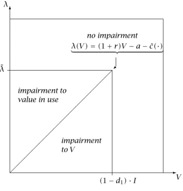
図
関連したドキュメント
Let X be a smooth projective variety defined over an algebraically closed field k of positive characteristic.. By our assumption the image of f contains
Many interesting graphs are obtained from combining pairs (or more) of graphs or operating on a single graph in some way. We now discuss a number of operations which are used
As explained above, the main step is to reduce the problem of estimating the prob- ability of δ − layers to estimating the probability of wasted δ − excursions. It is easy to see
This paper is devoted to the investigation of the global asymptotic stability properties of switched systems subject to internal constant point delays, while the matrices defining
In this paper, we focus on the existence and some properties of disease-free and endemic equilibrium points of a SVEIRS model subject to an eventual constant regular vaccination
Kilbas; Conditions of the existence of a classical solution of a Cauchy type problem for the diffusion equation with the Riemann-Liouville partial derivative, Differential Equations,
Related to this, we examine the modular theory for positive projections from a von Neumann algebra onto a Jordan image of another von Neumann alge- bra, and use such projections
Then it follows immediately from a suitable version of “Hensel’s Lemma” [cf., e.g., the argument of [4], Lemma 2.1] that S may be obtained, as the notation suggests, as the m A
