本文 Thesis 総合研究大学院大学学術情報リポジトリ A1716本文

(1)

A dissertation

submitted in partial fulfillment of the requirements for the degree Doctor of Philosophy

by

Md. Ashad Alam

in

Department of Statistical Science The Institute of Statistical Mathematics The Graduate University of Advanced Studies

Tokyo 190-8562, Japan.

September 2014

(2)

(3)

form for publication on microfilm and electronically.

Prof. Satoshi Kuriki

Dr. Shotaro Akaho

Prof. Daichi Mochihashi

Prof. Kenji Fukumizu Adviser

Prof. Koji Kanefuji

Department Head/ Director

September 2014

(4)

Our motherland Gônôprôjatôntri Bangladesh (The People’s Republic of Bangladesh)

(5)

Without Modern Mathematics Statistics, Robust Statistics and Statistical Machine Learning are like Gardening without any Flowers.

(6)

List of Tables

2.1 Examples of well-known positive definite kernels and its parameters. . . 23 3.1 Computational cost (in second) of the proposed method for synthesized

data-2 with different data sizes (n) and the numbers of components (ℓ) . . . 48 3.2 The configuration of datasets for hyperparmeters choice in kernel principal

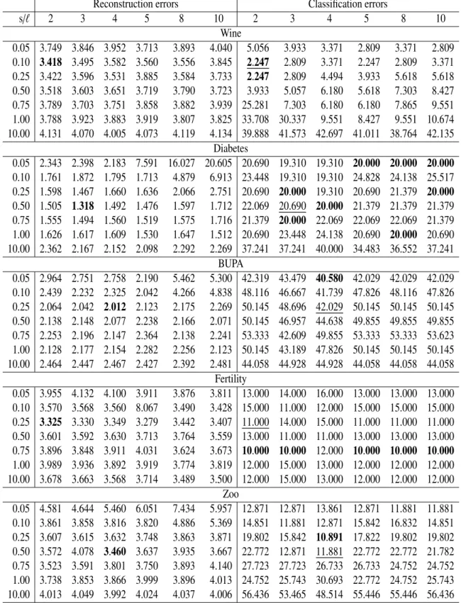
component analysis (kernel PCA). . . 50 3.3 Five real-world data sets: leave-one-out cross validation (LOOCV) recon-

struction errors and LOOCV classification errors for inverse bandwidths (s) and the number of components (ℓ). The minimum values are written in bold fonts, and the classification errors with the hyperparameters chosen by the proposed method are underlined. . . 55 3.4 USPSG-500: LOOCV reconstruction errors and LOOCV classification er-

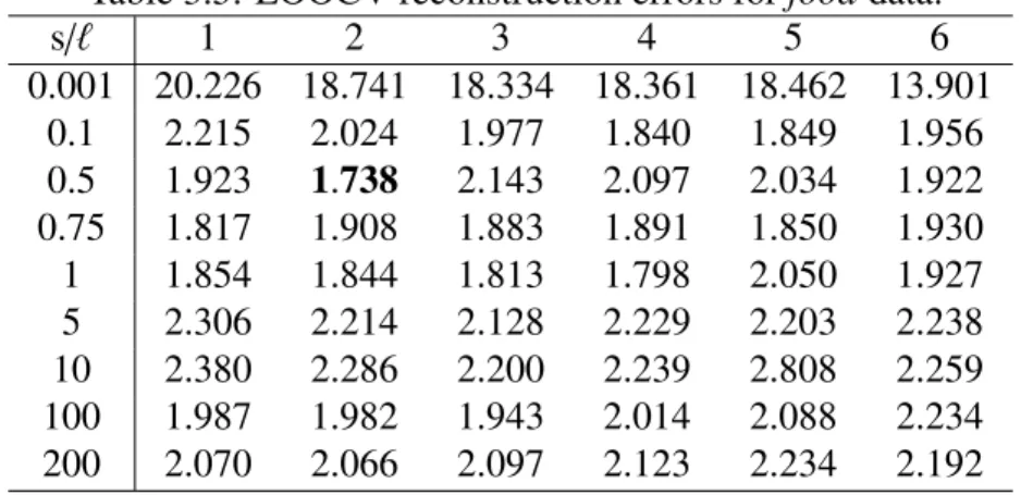
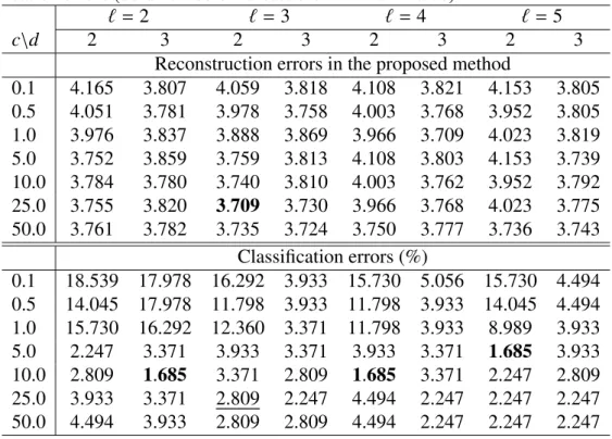
rors (bold numbers indicate the minimum value). . . 56 3.5 LOOCV reconstruction errors for food data. . . 56 3.6 Polynomial kernel for wine data: LOOCV reconstruction errors and the

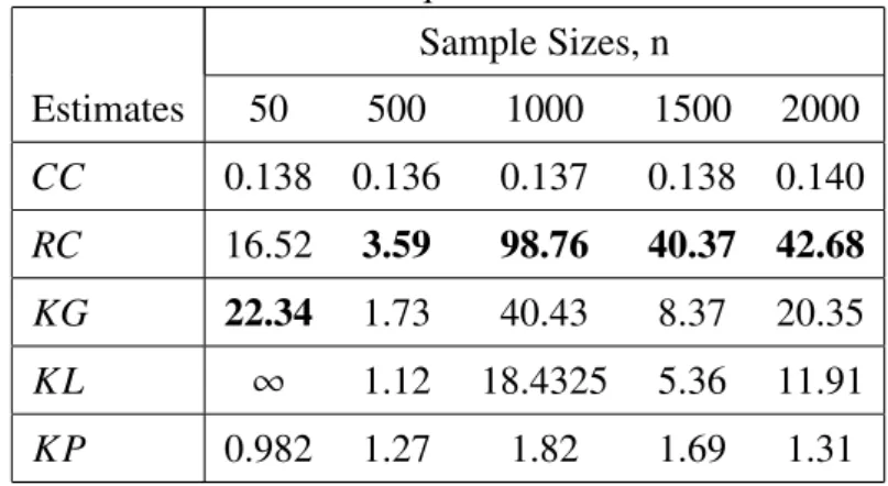
LOOCV classification errors (bold numbers indicate the minimum value). . 57 4.1 Bias and mean square error of simulated data (bold numbers indicate the

minimum value). . . 66 4.2 The value of qualitative robustness index. . . 66 5.1 Time complexity (in second) for example 3: the proposed kernel CCA with

three numbers of iterations (I) and the standard kernel CCA (KCCA). The Gaussian kernel is used for the both methods, and n is the sample size. . . . 84

(10)

feature (EDF), measure of association (MA) and estimate of low dimensional space (ELDS)) of all experimental datasets. . . 85 5.3 Cross-validation errors of the three examples (E₁ _{− E}₃) using different

inverse bandwidths s and regularization coefficients λ for the proposed method and standard kernel CCA (KCCA). . . 87 5.4 Cross-validation errors for nutrimouse dataset. . . 88 5.5 Classification errors (%) for wine, BUPA liver disorders and diabetes. One

or two dimensional features are used with the proposed method (hrKCCA+kNN and hrKCCA+SVM) and the kernel CCA. . . 91 5.6 Classification errors (%) using one dimensional estimated subspace of DB-

World subject and bodiesdatasets by the proposed method (hrKCCA+kNN and hrKCCA+SVM_L) other exiting methods. . . 93 5.7 Recognition rate (%) for KTH dataset (all scenarios) by the proposed method

(hrKCCA+kNN and hrKCCA+SVM_L) and other methods. . . 94 5.8 Recognition rate (%) for UMD dataset by the proposed method (hrKCCA+kNN

and hrKCCA+SVM_L) and some of the best stat-of-the-art methods of this dataset. . . 95

(11)

List of Figures

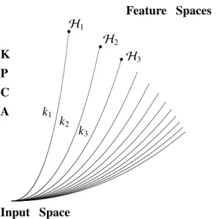
2.1 Background of the kernel in the 20th century. . . 16 3.1 Individual reproducing kernel Hilbert space for each kernel of the kernel

principal component analysis (KPCA). . . 44 3.2 Scatter plots of the first two kernel principal components for wine data:

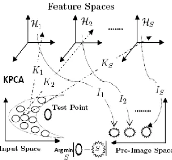
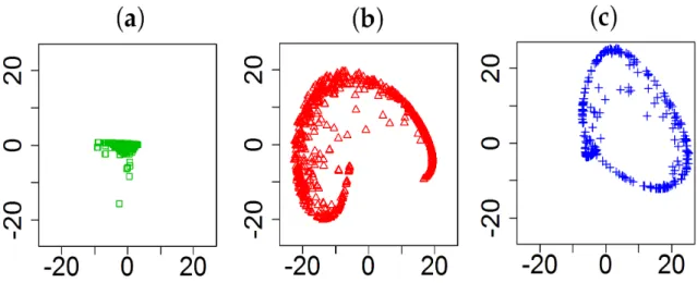
Gaussian RBF kernel is used in the top panel (a) s = 0.05 (b) s = 0.75 (c) s = 1 (d) s = 10, and polynomial kernel in the bottom (e) c = 0.001, d = 2 (f) c = 10, d = 2 (g) c = 1, d = 3 (h) c = 1, d = 4. . . 45 3.3 Architecture of kernel choice in kernel PCA. . . 48 3.4 Algorithm of kernel choice in kernel PCA with Gaussian RBF kernel. . . . 49 3.5 Kernel PCA for synthesized data-1 (top) and synthesized data-2 (bottom).

(a) Scatter plot for the two variables of a sample. (b) Box plots of the leave- one-out cross validation (LOOCV) reconstruction errors for 100 samples. (c, d) scatter plots of the first two kernel principal components using (c) the best inverse kernel widths (s = 5, 10) and (d) larger bandwidths s = 50, 200. 51 3.6 Visualization of the first two kernel principal components of food data (a)

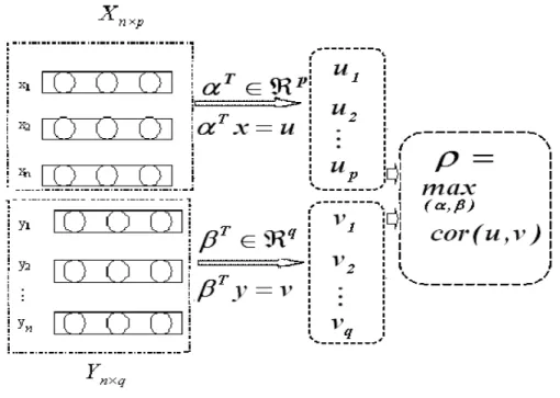
s =0.001, (b) s = 0.5 and (c) s = 200 . . . 53 4.1 The system of CCA. . . 60 4.2 The system of kernel CCA. . . 63 4.3 Box plots of canonical correlation coefficient of five estimators using pop-

ulation canonical correlation, PCC = 0.79 and PCC = 0.63. . . 67 4.4 Scatter plots of (X₁,Y₁) (top left) and first canonical variates . . . 68 4.5 Scatter plots of (X₂,Y₂) (top left) and 2nd canonical variates . . . 69

(12)

and b) transform multivariate normal data. . . 71 4.7 Breakdown plots for first canonical correlation coefficient. . . 73 5.1 Standard kernel CCA: the scatter plots of the 1st canonical variates for the

nutrimouse dataset (liver cells and hepatic fatty acids) using the Gaussian RBF kernel with eight inverse bandwidths s and fixed regularization coefficient κ = 10⁻⁴. The 10-fold cross-validation errors are also embedded. . . 78 5.2 Algorithm of the higher-order regularized kernel CCA. . . 83 5.3 Scatter plots of 1st kernel canonical variates for the examples (E₁_−E₃). The

first column for the standard kernel CCA. The final three columns for the hrKCCA, using different trade-off c for the regularization parameters: ν = cλ. The inverse bandwidth s and the 4th moment regularization coefficient λare chosen by the CV. . . 96 5.4 Box plots and line plots (inset) using mean values of cross-validation er-

rors of 100 samples for example 3 (bandwidths, s₁ = 225, s₂ = 250, s₃ = 275, s₄ =300, s₅= 325, s₆ =350, s₇ =375, s₈= 400). . . 97 5.5 Scatter plots of the 1st kernel canonical variates given by the proposed

method for the nutrimouse dataset (liver cells and hepatic fatty acids) using the Gaussian RBF kernel with eight inverse bandwidths s and fixed regularization coefficient λ = 0.75. The 10-fold cross-validation error is also embedded (see also Table 5.4). . . 98 5.6 Scatter plots of the first canonical variates of real datasets (Email (D₂),

Psychological (D₃) and Carbig (D₄)) using the parameters chosen by CV for the kernel CCA (a) and the proposed method (b). . . 99 5.7 Scatter plots of the first canonical variates (a(i)) -(d(i)) and the first two

canonical variates of the exploratory variables (a(ii) -d(ii)) for the wine dataset. The proposed method (s = 0.05, λ = 0.1) in (a) and kennel CCA using three heuristic bandwidths (s₁ = 0.02, s₂ = 0.073, s₃ = 0.05) in (b - d) are shown. . . 100

(13)

index plots (lower row) given by the proposed method for DBWorld subject, bodies, BUPA liver disorders, and diabetes. . . 101 5.9 Scatter plots of the first canonical variates (upper row) and the first two

canonical variates of X (lower row) using KTH dataset (outdoor scenario only) for the kernel CCA. . . 102 5.10 Scatter plots of the first canonical variates (upper row) and first two canon-

ical variates of X (lower row) using KTH dataset (outdoor scenario only) for the proposed hrKCCA. . . 103 5.11 Scatter plots of the first canonical variates (upper row), first two canonical

variates of X (middle row) and confusion matrices (lower row) using KTH dataset for all scenarios (boxing (B), hand clapping (HC), hand waving (HW), jogging (J), running (R), and walking (W)) for the for the proposed hrKCCA. . . 104

(14)

First and foremost, I would like to pay my thanks to my adviser, Professor Kenji Fukumizu, The Institute of Statistical Mathematics (ISM) and The Graduate University of Advanced Studies (SOKENDAI). I owe a great deal of gratitude to him for his guidance, financial support and help throughout the exciting journey full of learning and growth at my doctoral courses and research in Japan.

I would like to extend my thanks to the faculty members, especially Professor Shinto Eguchi, Professor Satoshi Ito, Dr. Yoichi Nishiyama who taught me during the doctoral courses. It’s my pleasure to thank to Dr. Osamu Komori. He served me as a family member in the last five years in Japan. I will keep them my mind always who had assisted me cordially in getting relevant literatures and other necessary advice.

I acknowledge to the staffs of ISM and research Cooperation Unit (Kenkyo) for their cordial help and co-operation during my research work. I am very grateful to Dr. Takao Kumazawafor his excellent guidance and sightseeing in Tokyo during first two years.

I would like to express my heartfelt gratitude to all Fukumizu’s lab members and friends who have supported me through the years and have made my time at ISM so enjoyable. In particular, I would like to thank Dr. Akifumi Notsu, Yuta Tanoue, Hisaki Ikebata and Katsuhiro Omaewith whom I share many unforgettable memories.

One thing I must confess, without the encouragement and care all though my life, of my parents Md. Shamsul Alam Akando and Mst. Helena Alam would be quite impossible to continue the doctoral course and research. I would like to thank all of my family members and relatives. My special thanks go my M.Sc. adviser, Professor Mohammed Nasser University of Rajshahi, who encourages a lot to begin my research.

At last, my deepest gratitude and love, of course, belongs to my wife, Mst. Shajia Afrin, my daughter, Asfia Alsaba and my son, Saffat Ashad for their unconditional love and help. They are one of my main sources of inspiration.

(15)

by

Md. Ashad Alam in

Department of Statistical Science The Institute of Statistical Mathematics The Graduate University of Advanced Studies

Tokyo 190-8562, Japan.

In kernel methods, choosing a suitable kernel is indispensable for favorable results. While cross-validation is a useful method of the kernel and parameter choice for supervised learning such as the support vector machines, there are no well-founded methods, have been established in general for unsupervised learning. We focus on kernel principal component analysis (kernel PCA) and kernel canonical correlation analysis (kernel CCA), which are the nonlinear extension of principal component analysis (PCA) and canonical correlation analysis (CCA), respectively. Both of these methods have been used effectively for extracting nonlinear features and reducing dimensionality.

As a kernel method, kernel PCA and kernel CCA also suffer from the problem of kernel choice. Although cross-validation is a popular method of choosing hyperparameters, it is not applicable straightforwardly to choose a kernel and the number of components in kernel PCA and kernel CCA. It is important, thus, to develop a well-founded method for choosing hyperparameters of the unsupervised methods.

In kernel PCA, it is not possible to use cross-validation for choosing hyperparameters because of the incomparable norms given by different kernels. The first goal of the dissertation is to propose a method for choosing hyperparameters in kernel PCA (the kernel and the number of components) based on cross-validation for the comparable reconstruction errors of pre-images in the original space. The experimental results of synthesized and real-world datasets demonstrate that the proposed method successfully selects an appropriate kernel and the number of components in kernel PCA in terms of visualization and classification errors on the principal components. The results imply that the proposed method enables the automatic design of hyperparameters in kernel PCA.

(16)

theoretically derived. One observation of their analysis is that kernel PCA with a bounded kernel such as Gaussian is robust in that sense the influence function does not diverged, while for kernel PCA with unbounded kernels for example polynomial the influence function goes to infinity. This can be understood by the boundedness of the transformed data onto the feature space by a bounded kernel. While this is not a result of kernel CCA but for kernel PCA, it is reasonable to expect that kernel CCA with a bounded kernel is also robust. This consideration motivates us to do some empirical studies on the robustness of kernel CCA. It is essential to know how kernel CCA is effected by outliers and to develop measures of accuracy. Therefore, we do intend to study a number of conventional robust estimates and kernel CCA with different functions but fixed parameter of kernel.

The second goal of the dissertation is to discuss five canonical correlation coefficients and investigate their performances (robustness) by influence function, sensitivity curve, qualitative robustness index and breakdown point using different type of simulated datasets. The final goal of the dissertation is to extract the limitations of cross-validation for the kernel CCA, and to propose a new regularization approach to overcome the limitations of kernel CCA. As we demonstrate for Gaussian kernels, the cross-validation errors for kernel CCA tend to decrease as the bandwidth parameter of the kernel decreases, which provides inappropriate features with all the data concentrated in a few points. This is caused by the ill-posedness of the kernel CCA with the cross-validation. To solve this problem, we propose to use constraints on the 4th order moments of canonical variables in addition to the variances. Experiments on synthesized and real world datasets including human action recognition for a robot demonstrate that the proposed higher-order regularized kernel CCA can be applied effectively with the cross-validation to find appropriate kernel and regularization parameters.

(17)

Chapter 1 Introduction

Methods using positive definite kernel (PDK), kernel methods play an increasingly promi- nent role to solve various problems in statistical machining learning such as, web design, pattern recognition, human action recognition for a robot, computational protein function perdition, remote sensing data analysis and in many other research fields. Due to the kernel trick and reproducing property, we can use linear techniques in feature spaces without knowing explicit forms of either the feature map or feature spaces. It offers versatile tools to process, analyze, and compare many types of data and offers state-of-the-art performance.

Nowadays, PDK has become a popular tool for the most branches of statistical machine learning e.g., supervised learning, unsupervised learning, reinforcement learning, non-parametric inference and so on. Many methods have been proposed to kernel methods, which include support vector machine (SVM, Boser et al., 1992), kernel ridge regression (KRR, Saunders et al., 1998), kernel principal component analysis (kernel PCA, Sch¨olkopf et al., 1998), kernel canonical correlation analysis (kernel CCA, Akaho, 2001, Bach and Jordan, 2002), Bayesian inference with positive definite kernels (kernel Bayes’ rule, Fukumizu et al., 2013), gradient-based kernel dimension reduction for regression (gKDR, Fukumizu and Leng, 2014), kernel two-sample test (Gretton, 2012) and so on.

During the last decade, unsupervised learning has become an important application area of the kernel methods. There are two most powerful tools of unsupervised kernel methods, namely kernel principal component analysis (kernel PCA) and kernel canonical correlation analysis (kernel CCA) (Sch¨olkopf et al., 1998, Akaho, 2001). Using these two methods, we are able to extract effective nonlinear features by high dimensional embedding of data

(18)

based on the reproducing kernel Hilbert space (RKHS). They have also closed connection with many unsupervised dimensional reductions and manifold learning techniques (Izen- man, 2008, Chapter 16). Kernel PCA and kernel CCA have been applied in different areas of statistical machine learning such as reduction of dimensionality, image processing, feature extraction, de-noising, statistical shape analysis, novelty detection, pre-processing of regression and classification (Mika et al., 1999, Kwok and Tsang, 2003, Arias et al., 2007, Zheng et al., 2010, Hardoon et al., 2004, Huang et al., 2009a, Alzate and Suykens, 2008). In all of the above areas, kernel PCA and kernel CCA have been used with an arbitrary choice of the kernel and the number of features. The results are in fact very sensitive to both the choice of the kernel and the number of features of RKHS. As a kernel method, kernel PCA and kernel CCA also suffer from the problem of kernel choice. To the best of our knowledge, however, a well-founded technique for choosing the parameters has not yet been established.

The cross-validation (CV) approach is popularly used for choosing parameters of kernel methods, such as the bandwidth parameter in Gaussian kernel, especially in supervised learning. For SVM, the cross-validation is one of the most popular and useful ways of choosing the kernel and parameters (Arlot, 2010, Woen and Perry, 2009, Stone, 1974). In the case of standard linear PCA, the algorithm can be formulated as minimization for self-regression with reduced rank, and cross-validation approaches have been proposed for choosing the number of components (Krzanowski, 1987, Wold, 1978). The k-fold CV has been used for classical CCA (Liang, 1995). Note that it is not possible to apply the leave-one-out CV (LOOCV) with canonical correlation value, since the correlation is not computable with one data. While the CV with the canonical correlation value has been used for choosing the bandwidth in kernel CCA (Suetani et al., 2006), where very dense data from a chaotic dynamics are discussed, it is not easy in general to obtain reliable canonical correlation values by the k-fold CV for small data points.

The result of kernel PCA obviously depends on the choice of the kernel. It is often the case that the kernel has some parameters like the popular examples shown in Table 2.1. In such a case, these parameters may have a strong influence on the results. To depict the influence, using wine dataset we show the plots of the first two kernel principal components with different values of inverse-bandwidth parameters in the Gaussian RBF kernel, and

(19)

degree and constant in the polynomial kernel (see Section 3.3 and Figure 3.2). From the figures, we see that in both the kernels the results of kernel PCA depend strongly on the parameters, and an appropriate choice is indispensable for the method to give reasonable low-dimensional representation of data.

In kernel CCA with Gaussian RBF kernel, we need to select a proper inverse bandwidth and a regularization parameter. It is also well known each hyperparameter has the influence on the result of kernel CCA. A guideline to select the regularization parameter has been proposed by Hardoon et al. (2004) and a heuristic technique has been also used for choosing the bandwidth (Hardoon and Shawe-Taylor, 2009).

It is known that CCA and kernel CCA can be regarded as an alternating regression problem (Breiman and Friedman, 1985, Shawe-Taylor and Cristianini, 2004). CV using correlations or prediction error depends on the data concentration. When the data are concentrated in only a few extreme points with perfect or nearly perfect correlations, on the one hand, the CV error will be very small which satisfies the objective of kernel CCA (maximum correlation of canonical variate) but on the other hand, the canonical variates do not follow any well-posed distribution. In classification problems, we can use CV based on classification rates, but the smallest classification error does not correspond to the high correlated features of kernel CCA, in general.

For kernel CCA, however, the cross-validation approach based on the prediction error does not necessarily choose a good parameter in general. We demonstrate this problem using an example of the nutrimouse dataset for the Gaussian RBF kernel (see the Chapter 5). In Figures 5.1 we show eight scatter plots of the first canonical variates using eight inverse bandwidths together with the cross-validation errors. As we see, the larger value of inverse bandwidth provides smaller error (≈ 0), but the solution are ill-posed: high correlation is achieved by the features with most data concentrating on a few points. This example illustrates that a straightforward application of cross-validation for choosing a kernel is not appropriate. It is expected that the variance constraints on the kernel CCA do not regulate sufficient for a large variety of nonlinearity given by different kernels.

Although cross-validation is a popular method for choosing hyperparameters, it is not applicable straightforwardly to choose a kernel of kernel PCA and kernel CCA. It is important, thus, to develop a well-founded method of designing a kernel of unsupervised

(20)

kernel methods. The main goal of the dissertation is to design a kernel and robustness for unsupervised kernel methods.

1.1 Designing kernel for unsupervised kernel methods

Selection of hyperparameters (kernel and the number of features) of kernel PCA is not a straightforward task because each kernel provides an individual norm in corresponding feature space. So, we are not able to choose them based on a performance with the norms of the feature spaces. In Chapter 3, we propose a method for choosing an optimum kernel and the number of features through the LOOCV based on pre-image performance, which is an approximate inverse image of a point in the feature space. To this ends, we extract the pre-image of a test point projected onto the subspace in RKHS using a pre-image method of each feature space. We then evaluate the reconstruction error based on this pre-image. As in the leave-one-out cross-validation, each data set is regarded as a test point and the average error is computed. The kernel and the number of features corresponding to the minimum error is chosen as the optimum ones.

As the kernel PCA, selection of the kernel and the number of features for kernel CCA is also a challenging problem. We are not able to extract the kernel CCA fruitfully by LOOCV. Canonical correlation analysis is the generalization of regression analysis with multiple response variables. So, it is possible to use mean square error like as regression analysis to apply LOOCV. By this result, we have observed that for small bandwidth of Gaussian RBF kernel, the most of data points are accumulated but for a few extreme points. In this situations, the CV error is very small. Moreover, the CV values highly to depends on bandwidth in finite samples.

Kernel CCA is given by the second order statistics (e.g., variance) of the canonical variates; this would suffice for a complete statistical description of a Gaussian distribution, but not in general. With the rich function classes given by positive definite kernels, we need much stronger constraint to regulate the canonical variate sufficiently to make the cross-validation applicable. The kernel CCA subject to the higher-order constraints is proposed to select the tuning parameters using the cross-validation technique. We demonstrate the effectiveness of the proposed higher-order regularized kernel CCA, combined with the

(21)

cross-validation, in measuring the relationship and extracting effective features for classification using various synthesized and real world problems (see Chapter 5).

1.2 Robustness of unsupervised kernel methods

The influence function (IF) of kernel PCA has been theoretically well-known. Kernel PCA with a bounded kernel such as Gaussian is robust in the sense that the influence function does not diverge, while it is not robust with unbounded kernels for example polynomial (IF goes to infinity). This can be understood by the boundedness of the transformed data onto the feature space by a bounded kernel (Huang et al., 2009b, Suykens et al., 2010). While this is not a result of kernel CCA, it is reasonable to expect that kernel CCA with a bounded kernel is also robust. This consideration motivates us to do some empirical studies on the robustness of kernel CCA. It is essential to know how kernel CCA is affected by outliers and to develop measures of accuracy. Therefore, we intend to study a number of conventional robust estimates and kernel CCA with different functions, but fixed bandwidth of Gaussian RBF kernel and Laplacian kernel (see Chapter 4).

1.3 Scope of the research

Kernel PCA and kernel CCA are most useful and fundamental unsupervised statistical pattern recognition techniques as well as preprocessing techniques for supervised learning: regression analysis and classification analysis to predict from massive amounts of data. Both of these techniques are also used in unsupervised learning to extract significant and anomaly structure of high dimensional datasets. Kernel CCA is also used as a constrast function of independent component analysis, an important method of unsupervised learning. An additional important application area of kernel CCA is stochastic processes to learn the dynamic nature of the processes. The proposed two methods provide a way of automatic findings the hyperparemtes of the kernel PCA and kernel CCA. It is expected that our research would be a great impact on the area of statistical machine learning.

(22)

1.4 Outline and summary of the contributions

Chapter 1: The motivation of designing the kernel and robustness for unsupervised kernel methods are presented in the first chapter.

Chapter 2: A review of important and useful results of functional analysis and PDK is given in this chapter.

Chapter 3: This chapter discusses the limitations of kernel PCA and provides a new method for choosing hyperparameters in kernel PCA (kernel and the number of components) based on CV for the comparable reconstruction errors of pre-images in the original space. The proposed method has been applied to synthesized and a number of real world datasets.

Chapter 4: This chapter treats the performances of five canonical correlation coefficients in the different types of distribution using influence function, sensitivity curve, qualitative robust index and breakdown point.

Chapter 5: This chapter discusses the CV for kernel CCA with its limitations, and provides a new 4th order moment regularization approach for kernel CCA. The proposed method demonstrates for synthesized and real world problems, including human action recognition for a robot.

Chapter 6: A conclusion and further aspects of research are discussed in the final chapter.

(23)

Chapter 2 Preliminary of Functional Analysis and

Kernel

Functional analysis is an abstract branch of mathematics where the vector spaces are in general infinite dimensional and not all operators on them can be represented by matrices unlike the linear algebra. An abstract approach starts with a set of elements satisfying certain axioms. For example, in linear algebra we use it in connection with fields, rings and groups, but in functional analysis it in connection with abstract spaces (inner product space, Hilbert spaces, Banach spaces etc.,). An abstract space is a set (unspecified) of elements satisfying certain axioms. The different sets of axioms provide different abstract spaces.

Functional analysis has a history of more than one century and nowadays its results have been used in a number of areas: mathematics, statistics, robust statistics and statistical machine learning. Some basic definitions and results are summarized in this chapter, which are frequently used to reproducing kernel Hilbert space (RKHS) and its methods. The fundamental references of this chapter are: Hille (1972), Reed and Simon (1980), Kreyszig (1989), Cucker and Smale (2002), Sch¨olkopf and Smola (2002), Berlinet and Thomas- Agnan (2004), Shawe-Taylor and Cristianini (2004), Bishop (2006), Steinwart and Christ- mann (2008), Hofmann et al. (2008), G¨artner (2008), Fukumizu et al. (2009), King (2009), Fasshauer (2011), Steinwart and Scovel (2012) and Fukumizu et al. (2013).

(24)

2.1 Inner product space

In calculus, the notions of convergence and continuity can be formulated in terms of distance between two numbers or between two vectors, where the objects are very simple (R or Rⁿ). In functional analysis, we consider more general spaces, which contain more complicated objects than numbers and vectors e.g., functions and so on. To find a distance between two complicated objects, we need a new notion of distance that lead a new notion of convergence and continuity. These again lead to new arguments surprisingly similar to those we have already seen in calculus. Now the question, is it possible to develop a general theory of distance where we can prove the results (we need once and for all)? We have a positive answer and the theory is called the theory of metric spaces. By inducing general conditions on the distance function, we are able to develop a general notion of distance, which can be applicabled even on complicated objects. Using metric space theory, we can formulate and prove results about convergence and continuity once and for all.

Metric space is a set with a metric on it. We can generalize it by a notion of nearness (open set is sufficient). Simply imagine small open balls around a point to measure nearness without mentioning distances, which leads to the idea of a topological space. The fundamental notion of topological space is based on the collection of all open sets (complement is closed set) instead of metric. The field of topology is an abstract study that evolved as an independent discipline in response to certain problems of classical analysis and geometry. It provides a unifying theory that can be used in many diverse branches of mathematics.

The metric and topology are defined on an abstract set, which may or may not be a vector space. To make a relation between algebraic and geometric properties of an abstract set, we need to define a metric in the special form, say norm. A norm is nothing but a metric on the vector space, which is combined the algebraic structure and metric concepts. It can be given more useful and important metric spaces (Kreyszig, 1989).

In a normed space we can do vector addition and scalar multiplication of a vector just like the elementary vector algebra, but still we cannot do two useful operations: vector dot product and orthogonality of two vectors. It is possible to fill this gap using the inner product. A vector space together with an inner product is called an inner product space.

Definition 2.1.1 (Inner product space) Let V is a vector space (real or complex). The

(25)

inner product of the V is a continues mapping ⟨, ⟩ : V × V → F, that has the following four properties, where F is a scaler field of V:

CI1 (Positive definite)

⟨x, x⟩ ≥ 0, ⟨x, x⟩ = 0 ⇔ x = 0.

CI2 (Anti-symmetric (Hermitian))

⟨x, y⟩ = ⟨y, x⟩, ∀ x, y ∈ V.

For a real vector space (Symmetric).

⟨x, y⟩ = ⟨y, x⟩, ∀ x, y ∈ V.

CI3 (Homogeneity)

⟨ax, y⟩ = a⟨x, y⟩, ∀a ∈ F.

CI4 (Cumulative (addition))

⟨x + y, z⟩ = ⟨x, z⟩ + ⟨y, z⟩, ∀x, y, z ∈ V.

The pair(V, ⟨, ⟩) is called inner product space.

A metric is a measure of how different the elements of a set are. A norm is a measure of how large the element is. An inner product is a measure of what degree the elements are linearly independent.

A useful property of inner products is the Cauchy-Schwarz inequality,

⟨x, y⟩ ≤ ⟨x, x⟩¹²⟨y, y⟩¹²^. ^(2.1)

This relationship is also sometimes called the Cauchy-Bunyakovskii-Schwarz inequality.

(26)

2.2 Hilbert space

Hilbert spaces are possibly-infinite-dimensional analogues of the finite-dimensional Eu- clidean spaces familiar to us. In particular, Hilbert spaces have inner products, so notions of perpendicularity (or orthogonality) and orthogonal projection are available. Reasonably enough, in the infinite-dimensional case we must be careful not to extrapolate too far based only on the finite-dimensional case. Perhaps strangely, few naturally-occurring spaces of functions are Hilbert spaces.

Definition 2.2.1 (Hilbert space) A Hilbert space is a real or complex inner product space that is complete under the inner product.

Example 2.2.1 (Sequence spaces) The space ℓ²is a Hilbert space (real valued) with inner product defined as

⟨x, y⟩ =

∑∞ i=1

ξiνi, _{x, y ∈ ℓ}².

Example 2.2.2 Let H is a finite dimensional real vector space of functions with basis ( f₁, f₂,_{· · · , f}n). Any vector of H can be defined as a linear combination of ( f¹^, ^f²^,· · · , fⁿ⁾ in unique way. An inner product ⟨, ⟩H on H is define by the numbers

ki j ⁼_{⟨ f}i, fj_⟩, i, j =1, 2, 3, · · · , n.

If u₁ = ^∑ⁿ_i=1u_1ifi and u₂ =^∑ⁿ_j=1u_{2 j}fj, then

⟨u1^,^u2⟩H ⁼⟨

∑n i=1

u_1ifi,

∑n j=1

u_{2 j}fj_⟩_H ⁼

∑n i=1

∑n j=1

u_1iu_{2 j}ki j.

The matrix K = (k_{i j}) is called the Gram matrix of the basis. It is a positive definite matrix. A finite dimensional space endowed with any inner product is always complete and therefor it is a Hilbert space.

Example 2.2.3 (Lebesgue spaces) Given µ a Lebesgue measure on the set R of real numbers and L(a, b) (−∞ ≤ a ≤ b ≤ ∞, abstract set) be the set of all complex measurable

(27)

function over(a, b) such that

∫ b a ^{| f (t)|}

2dµ(t) < ∞.

Identifying two functions f₁and f₂of L(a, b) which are equal expect on a set of Lebesgue measure equal to zero, we get a Hilbert space,L(a, b) with inner product

⟨ f¹^, ^f²⟩^L(a,b)⁼

∫ b a

f₁(t) f₂(t)dµ(t).

Two (or more) Hilbert spaces can be combined to produce another Hilbert space by taking either their direct sum or their tensor product (new Hilbert spaces from old).

Definition 2.2.2 (Orthogonal complement) Let H is a Hilbet space and V of be a closed subspace H then

V^⊥:^{x_{∈ H} ⟨x, y⟩ = 0, ∀y ∈ V^}

is closed subspace and called the orthogonal complement of V.

Definition 2.2.3 (Orthogonal projection) Let H is a Hilbert space and V be a closed subspace. Every x ∈ H can be uniquely decomposed

x = y + z, y_{∈ V, z ∈ V}^⊥i.e., H = V ⊕ V^⊥^,

which is called orthogonal projection.

Definition 2.2.4 (Complete orthonormal system) A subset {vⁱ}i∈I of H is called an orthonormal system (ONS) if ⟨vⁱ^{, v}^j⟩ = δ^{i j} ^(δ^{i j} is Kronecker’s delta). It is called complement orthonormal system (CONS) or orthonormal basis if it is ONS and if

⟨x, v^j⟩ = 0, (∀i ∈ I) ⇒ x = 0, ∀x ∈ H.

Facts 2.2.1 Any ONS in a Hilbert space can be extended to a CONS.

Definition 2.2.5 (Separable Hilbert space) A Hilbert space is separable if it has a count- able CONS.

(28)

Theorem 2.2.1 (Fourier series expansion, (Kreyszig, 1989)) _{Let {v}_i_}^∞_i=1 is a CONS of a separable Hilbert space. For each x ∈ H,

x =

∑∞ i=1

⟨x, vⁱ⟩vⁱ (Fourier expansion)

||x||² ⁼

∑∞ i=1

|⟨x, vⁱ⟩|² (Parseval’s equality).

For a general orthonormal system, the Parseval’s equality becomes a Bessel inequality

||x||² ≥

∑∞ i=1

|⟨x, vⁱ⟩|²^.

2.3 Feature space and its drawback

In the beginning (1980s) of statistical machine learning the main goal was not inference (estimation) but generalization or a good “predictive” capability Hastie et al. (2009), Sch¨olkopf and Smola (2002). However, some nonparametric inference methods have been also devel- oped for inference Fukumizu et al. (2013), Gretton (2012), and so on. For generalization or a good prediction, We seek to arrive at a function

f _{: X → Y}

based on training data, {(x1^{, y}1^{), (x}2^{, y}2), . . . (x_n, yn)}. The goal, a given test set {x^′i}^ti=1^{, arrive}

at “good” predictions {y^′i}^t_i=1via f . Define the hypothesis space H as the space of functions to consider for f . The learning problem can then be summarized as finding a method L that maps a training set to a function of the hypothesis space:

L_{: (X × Y)}ⁿ _{→ H.}

Define an unknown probability measure on X and Y : µ(dx, dy) but assume that the training samples {(xⁱ^{, y}ⁱ)} ∼ p(x, y) is independent and identically distributed (iid).

We need some measure of “similarity” between elements of the input space X via inner

(29)

product space (tractable learning problem). For this purpose, we need a function that takes any pair of values x ∈ X and x^′ ∈ X a real value returns their “similarity”:

k: X × X → R, (x, x^′) → k(x, x^′^),

where k refers to as a kernel. This allows us to make statements about how similar the outputs y with new y^′. Similarity measure by inner product

⟨x, z⟩ = Large if x and z similar

= Small if x and z different

For example, Good measure how similar x, z

k(x, x^′) = e⁻^2s2¹ ^∥x−x^′^∥²; k(x, x^′) = ⟨^{x, x}^′^⟩

∥x∥∥x^′∥^.

We have to seek a space that incorporates inner product by map X into a new space with some additional structure. Do linear techniques work in nonlinear inputs space? The answer is negative.

Definition 2.3.1 (Input space) The space of all original data is called input space. The representation space is the set of all possible object descriptions that can occur in a given problem.

The following basic linear techniques do not work well in nonlinear input space:

• Correlation analysis,

• Linear regression analysis,

• Fisher discriminant analysis,

• Principal component analysis (PCA),

• Canonical correlation analysis (CCA) and so on.

So we need to seek a new space for which linear techniques are worked well, say feature space.

(30)

2.3.1 Feature space

Definition 2.3.2 (Feature space) Let X is a set and x ∈ X

Φ:= X → H, x → Φ(x)

is a feature map and the vector Φ(x) in H is called feature vector. The space H for all functions via Φ is called feature space. It is a finite or infinite dimensional vector space.

For example, let X ∈ R be the variable for the duration of earthquake in last two months.

X →





 ϕ₁(X) ϕ2^(X)

ϕ₃(X) ϕ4^(X)







=





 X X² X³ X⁴







= Φ(X), ϕi’s are the nonlinear maps.

The map X → H not for only similarity, but also has more features:

• induce a geometric structure that we can leverage (deal with the patterns geometri- cally),

• linearizing of nonlinear space (linear, but nonlinear in input space),

• the freedom to choose the mapping Φ will enable us to design a large variety of learning algorithms.

The main argument is that any low-dimensional structure may be more easily discov- ered when it becomes embedded in the larger space H, which could be infinite dimensional space.

2.3.2 Computational problems of feature space

For high dimensional feature vector Φ(X), we are not able to compute the inner product

⟨Φ(X), Φ(X)⟩. For example, simple, bivariate case up to quadratic transforms

X =(X, Y) → (X, Y, X²^,^Y²^,^XY)

(31)

We have five variables to use linear method (R⁵). If we consider 3 variables and higher oder up to cubic transforms

X =(X, Y, Z) → (X, Y, Z, X²^,^Y²^,^Z²^,XY, XZ, YZ, X²Y, X²Z, XYZ . . .).

If the input vector X is 100 dimensional and the moments up to the 4th order are used (100

1 )

+⁽¹⁰⁰ 2

)

+⁽¹⁰⁰ 3

)

+⁽¹⁰⁰ 4

)

= 4087975 = dim(H).

Computational cost will be expensive on the inner product of the feature space and impossible for infinite dimension.

2.4 Kernel and positive definite kernel

2.4.1 Kernel

The term kernel has a long history. The meaning of the kernel depends on the subjects that has different meanings in different literatures. In mathematics, the term kernel itself is used with different meanings, for example, in linear algebra where it is used as a synonym for the null space. In the beginning of the last century David Hilbert and other researches, the term kernel has been used as a bivariate function to the field integral operators. The term kernel has been also used for density estimation in the statistical literature, where the kernel K : R → R is an integrable function satisfying^∫ K(x) dx = 1.

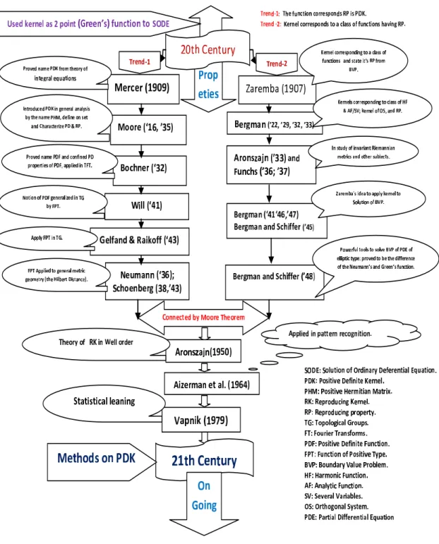
The term kernel has been also used as a positive definite kernel (PDK) in the branch of mathematics since 1950s. The PDK is a large class of kernels, which contains Mercer kernel and so on. It can be regarded as a generalized dot product. Figure 2.1 presents the historical background of the kernel in the 20th century.

(32)

Figure 2.1: Background of the kernel in the 20th century.

Definition 2.4.1 (Kernel) Let X be a non-empty arbitrary set. A bivariate function k : X × X → R is called kernel on X if there exists a Hilbert space, H and a feature map Φ: X → H such that for all x, x^′ ∈ X we have

k(x, x^′) = ⟨Φ(x), Φ(x^′)⟩.

(33)

In general the kernel may be also defined on the complex field. So, Hilbert space may be also a complex valued Hilbert space.

Algorithms can be applied in dot product space by considering the kernel as a similarity measure. We can construct a kernel of several ways as follows:

• straightforward construction of feature map and space,

• using a sequence of functions ( fⁿ : X → F, n ∈ N such that ( fⁿ^(x))^∞n=1) ∈ ℓ²^, ∀x ∈ X,

• using algebraic properties of the set of kernels, k1^{and k}2^,

– sum of kernels on same set (k₁+k₂),

– scalar multiplication of kernel (αk)< 0, α_{∈ F,} – product of kernel on different set, k₁k₂

– polynomial of kernel with positive coefficients, – taking exponential,

• using Taylor series,

• using Fourier series,

• pointwise limit of kernels.

We can define a number of feature maps via a kernel as follows.

• Aronszajn map: Φ : x → k(x, ·), H^k is the associated reproducing kernel Hilbert space (RKHS) k(x, y) = ⟨k(x, ·), k(y, ·)⟩.

• Kolmogorov map: Φ : x → Xx^, H^k ⁼ ^L2^(R^X, µ), where µ is the Gaussian measure k(x, y) = E[X_xX_y].

• Integral map: there exists a set T and a measure µ such that on has Φ : x → (Γ_x(t))_t∈T,_Hk ⁼ L₂(T, µ), k(x, y) =^∫ Γ(x, t)Γ(y, t)dµ(t).

• Basis map: given any orthonormal basis ( fα⁾α∈I of the RKHS associated with H, on has Φ : x → ( f^α⁾^α∈I^,H = ℓ²(I) and k(x, y) = ∑_α_∈I f_α(x) f_α(y).

When infinite sums are involved like in the Basis map, it is important to specify in which sense the sum converges. In general the convergence occurs for each pair.

(34)

2.4.2 Advantages of kernel

It is well-known that the feature space suffers the computational problem. In case of high dimensional data the computational cost becomes very high. Using inner product by the kernel we can overcome this problem efficiently. First advantage of the kernel is that in many important special case feature computation will be very inexpensive by k(x, z) =

⟨Φ(x), Φ(z)⟩, where x and z are in the arbitrary set X. Example 2.4.1 (Quadratic kernel) Let x, z ∈ R^m^{we have}

k(x, z) = [x^Tz]² =(

∑m i=1

xizi)(

∑m j=1

xjzj) =

∑m i=1

∑m j=1

(xixj)(zizj) = ⟨Φ(x), Φ(z)⟩.

In case m =3

Φ(x) =





 ϕ₁(x) ϕ₂(x) ϕ₃(x) ϕ₄(x) ϕ₅(x) ϕ₆(x) ϕ₇(x) ϕ₈(x) ϕ₉(x)







=





 x₁x₁ x₁x₂ x₁x₃ x₂x₁ x₂x₂ x₂x₃ x₃x₁ x₃x₂ x₃x₃







Cost for kernel, k(x, z) = O(m) is linear but for ϕ(x) = O(m²) is quadratic.

Example 2.4.2 (Polynomial kernel) Let x, z ∈ R^musing polynomial kernel we have

k(x, z) = [x^Tz +c]² = _{⟨x, z⟩}²+_{2c⟨x, z⟩}²+c²= ⟨Φ(x), Φ(z).⟩

(35)

In case m =3

Φ(x) =





 ϕ₁(x) ϕ₂(x) ϕ₃(x) ϕ₄(x) ϕ₅(x) ϕ₆(x) ϕ₇(x) ϕ₈(x) ϕ₉(x) ϕ₁₀(x) ϕ₁₁(x) ϕ₁₂(x) ϕ₁₃(x)







=





 x₁x₁ x₁x₂ x₁x₃ x₂x₁ x₂x₂ x₂x₃ x₃x₁ x₃x₂ x₃x₃

√2cx₁

√2cx₂

√2cx₃ c







In general dim(H) = ⁽^m+dd

) different features consisting all monomials having degree at most d with input dimension m.

The second advantage of the kernel is to use non-vectorial data, e.g., text strings or DNA sequences and so on. Another important advantage is that given a kernel we need neither the explicit form of the feature map nor the feature space, which are not also uniquely determined. Moreover, note that a similar construction can be made for arbitrary kernels and consequently every kernel has many different feature spaces. However, we can always construct a canonical feature space, namely the RKHSs (see Section 2.5). RKHSs have the remarkable and important property that norm convergence implies pointwise convergence.

2.4.3 Positive definite kernel (PDK)

Although we have already seen several techniques to construct kernels, in general, we still have to find a feature space in order to decide whether a given function k is a kernel or not. Since this can sometimes be a difficult task, we will now present a criterion that characterizes R-valued kernels in terms of inequalities (positive semi-definite). By the

(36)

definition of positive definite function, if k is a R-valued kernel with feature map Φ : X → H. The kernel k is symmetric since the inner product in H is symmetric. Moreover, k is also positive definite since for n ∈ N, α1^{, α}2, . . . , αn _{∈ R and x}1^,· · · , xⁿ ∈ X

∑n i=1

∑n j=1

αiαjk(xi, xj_{) = ⟨}

∑n i=1

αiΦ(xi),

∑n j=1

αjΦ(x^′_j_)⟩_H _{≥ 0.}

We can check whether a bivariate function is PDK by symmetry and positiveness.

Definition 2.4.2 (Kernel matrix or Gram matrix) Given a kernel k and inputs x₁,_{· · · , x}_n_∈ X, the square matrix

K := (k(xi, xj))i, j

of order n is called the kernel matrix (Gram matrix) of k with respect to x₁,_{· · · , x}n. Definition 2.4.3 (Positive semi-definite matrix) A real symmetric matrix K satisfying

∑n i=1

∑n j=1

αiαjKi j _{≥ 0, ∀α}i _{∈ R} (2.2)

is calledpositive definite kernel. It is said to be strictly positive definite if equality in (2.2) occurs for α₁ = α₂ =_{· · · = α}_n =0.

Definition 2.4.4 (Positive definite kernel) A symmetric kernel k(·, ·) defined on a non-empty space X is called positive definite if for arbitrary number of points x1, . . . , xn∈ X the kernel matrix(k(xi, xj))ⁿ_{i, j=1}is positive semi-definite.

In kernel methods, the nonlinear feature map is given by a positive definite kernel, which provides nonlinear methods for data analysis with efficient computation. It is known that a positive definite kernel k is associated with a Hilbert space H, called reproducing kernel Hilbert space (see Section 2.5), consisting of functions on X so that the function value is reproduced by the kernel (Aronszajn, 1950).

Definition 2.4.5 (Reproducing property) For any function of RKHS, i.e., f ∈ H and a point x ∈ X, the function value f (x) is given by

f(x) = ⟨ f (·), k(·, x)⟩H^, ^(2.3)

(37)

where ⟨, ⟩H in the inner product of H, which is called reproducing property.

The reproducing property says that each Dirac functional can be represented by the reproducing kernel. A Hilbert function space H that has a reproducing kernel k is always a RKHS (see Section 2.5). Every RKHS has a (unique) reproducing kernel and that this kernel can be determined by the Dirac functionals.

Definition 2.4.6 (Kernel trick) By replacing f with k(·, ˜x) in Eq. (2.3) yields

k(x, ˜x) = ⟨k(·, x), k(·, ˜x)⟩H for any x, ˜x ∈ X.

To transform data for extracting nonlinear features, the feature map Φ : X → H is defined by

Φ(x) = k(·, x),

which is regarded as a function of the first argument. The inner product of two feature vectors is then given by

⟨Φ(x), Φ(˜x)⟩H ⁼ ^{k(x, ˜x).}

This is known as thekernel trick.

The kernel trick serves as a central equation in the kernel methods. By this trick the kernel can evaluate the inner product of any two feature vectors efficiently without knowing an explicit form of neither Φ(·) nor H. With this computation of inner product, many linear methods of classical data analysis techniques can be extended to nonlinear ones with an efficient computation based on Gram matrices. Once Gram matrices are computed, the computational cost does not depend on the dimensionality of the original space.

2.4.4 Well-known PDKs and its parameters

Assume k : X × X → R is positive definite kernel. Then for any x, x^′ ∈ X, the following kernels are real valued positive definite kernels on R:

(38)

i. Linear kernel

k₀(x, x^′_{) = ⟨x, x}^′_{⟩ = x}^Tx^′.

It is just used the underlying Euclidean space to define the similarity measure. When- ever the dimensionality of x is very high, this may allow for more complexity in the function class than what we could measure and assess otherwise. It has limitation of linearity.

ii. Polynomial kernel

kP(x, x^′) = (x^Tx^′+c)^d, (c ≥ 0, d ∈ N).

Using polynomial kernel it is possible to use the higher order correlation between the data in the different purposes. This kernel incorporates all polynomial interactions up to degree d (provided that c > 0). For instance, if we wanted to take only mean and variance into account, we would only need to consider d = 2 and c = 1. For higher emphasis on mean we need to increase the constant offset a. Polynomial kernels only map data into a finite dimensional space. Due to the finite bounded degree such kernel will not provide us with guarantees for a good dependency measure.

iii. Gaussian radial basis function (RBF) kernel

kG(x, x^′) = e^−s||x−x^′^||², (s > 0).

Many radial basis function kernels, such as the Gaussian RBF kernel map x into an infinite dimensional space.

iv. Exponential kernel

kE(x, x^′) = e^(αx^T^x^′⁾, (α > 0).

(39)

v. Laplacian kernel

kL(x, x^′) = e^{−β∥x−x}^′^∥, (β > 0).

• Binomial kernel: Let X := {x ∈ R^d : ∥x∥² ^<1} and α > 0. Then

k(x, x^′) := (1 − ⟨x, x^′⟩)^−α^.

Table 2.1: Examples of well-known positive definite kernels and its parameters.

Kernel k(x, ˜x) Parameter

Polynomial (⟨x, ˜x⟩ + c)^d c ≥ 0, d ∈ N Gaussian RBF e^{−s||x−˜x||}² s >0 Exponential e^(αx^T^˜x) α >0 Laplace e^{−β∥x−˜x∥} β > 0

Definition 2.4.7 (Stationary kernels) Let κ : Rⁿ → R be a function. Then κ is called a positive definite function (or function of positive type or Stationary kernels) if

k(x, z) = κ(x − z)

this type of the kernel is called stationary, a stationary kernel. It depends only on the lag vector separating the two examples x and z but not on the examples themselves. A stationary kernel of the form ϕ(x−y) is also called a shift invariant (or translation invariant) kernel. Gaussian and Laplacian kernels are example of stationary kernel.

Definition 2.4.8 (Nonstationary kernels) A kernel is called nonstatinary, which depends on explicitly on the two examples x and z of k(x, z) . For example Linear kernel and polynomial kernel.

(40)

2.4.5 Valid PDKs and its matrices

Given an arbitrary set X. Assume there exist Φ such that k(x, x^′) = ⟨Φ(x), Φ(x^′)⟩ (kernel trick) is a valid PDK, where x , x^′ _{∈ X. Let x}₁, x₂, . . . , xn _{∈ X and c}1^,^c2^{, . . . ,}^cn_{∈ R. Then}

∑n i=1

∑n j=1

cicj^k(xi, xj^{) =}

∑n i=1

∑n j=1

cicj_⟨Φ(xi^{), Φ(x}j_{)⟩ = ⟨}

∑n i=1

ci^Φ(xi^),

∑n i=1

cj^Φ(x)j_{⟩ = ||}

∑n i=1

ci^Φ(xi_)||² _{≥ 0}

i.e. the symmetric matrix

K = (k(x_i, xj⁾⁾ⁿ_{i, j=1} ⁼







k(x₁, x₁) k(x₁, x₂) . . . k(x₁, xn⁾

k(x₂, x₁) k(x₂, x₂) . . . k(x₂, xn) ... ^... . . . ^... k(xn, x₁) k(xn, x₂) . . . k(xn, xn)







is positive semidefinite. The kernel matrix K = (k(x_i, xj⁾⁾ⁿ_{i, j=1}is often called a Gram matrix in statistical machine learning literature. Symmetry an positive definiteness are not only necessary for k to be a PDK but also sufficient.

We do not actually need to have a centered Φ but for some methods we do need K

˜Ki j ⁼ _{⟨ ˜Φ(x}i), ˜Φ(xj_{)⟩ = ⟨Φ(x}i_{) −} ¹

n

∑n a=1

Φ(xa), Φ(xj_{) −} ¹

n

∑n b=1

Φ(xb_)⟩

= _⟨Φ(x_i), Φ(x_j_{)⟩ −} ¹ n

∑n b=1

⟨Φ(xⁱ^{), Φ(x}^b)⟩ − ¹_n

∑n a=1

⟨Φ(X^a^{), Φ(x}^j)⟩ + _n¹₂

∑n a=1

∑n b=1

⟨Φ(x^a^{), Φ(x}^b)⟩

= Ki j₋

1 n

∑n b=1

Kib₋

1 n

∑n a=1

Ka j⁺

1 n²

∑n a=1

∑n b=1

Kab

= Ki j₋

1 n

∑n b=1

Kib¹b j₋

1 n

∑n a=1

1_iaKa j⁺

1 n²

∑n a=1

∑n b=1

1_iaKab¹b j

= _{(K − K(n}⁻¹Jn_{) − (n}⁻¹Jn)K + (n⁻¹Jn)K(n⁻¹Jn))i j,

= (HKH)i j (2.4)

where for all i and j, 1_{i j} =1, 1_n =[1, 1, · · · , 1]^T, and H = I_n₋ _n¹J_nwith J_n =1_n1^T_n.

本文 Thesis 総合研究大学院大学学術情報リポジトリ A1716本文

Contents

List of Tables

List of Figures

Chapter 1

Introduction

1.1 Designing kernel for unsupervised kernel methods

1.2 Robustness of unsupervised kernel methods

1.3 Scope of the research

1.4 Outline and summary of the contributions

Chapter 2

Preliminary of Functional Analysis and

Kernel

2.1 Inner product space

2.2 Hilbert space

2.3 Feature space and its drawback

2.3.1 Feature space

2.3.2 Computational problems of feature space

2.4 Kernel and positive definite kernel

2.4.1 Kernel

2.4.2 Advantages of kernel

2.4.3 Positive definite kernel (PDK)

2.4.4 Well-known PDKs and its parameters

2.4.5 Valid PDKs and its matrices